A MODEL FOR THE THERMOELASTIC BEHAVIOR OF A
JOINT-LEG-BEAM SYSTEM FOR SPACE APPLICATIONS
E.M. CLIFF, Z. LIU, AND R. D. SPIES∗
Abstract. Rigidizable-Inflatable (RI) materials offer the possibility of
de-ployable large space structures (C.H.M. Jenkins (ed.), Gossamer Spacecraft: Membrane and Inflatable Structures Technology for Space Applications, Pro-gress in Aeronautics and Astronautics, 191, AIAA Pubs., 2001) and so are of interest in applications where large optical or RF apertures are needed. In particular, in recent years there has been renewed interest in inflatable-rigidizable truss-structures because of the efficiency they offer in packaging during boost-to-orbit. However, much research is still needed to better under-stand dynamic response characteristics, including inherent damping, of truss structures fabricated with these advanced material systems. One of the most important characteristics of such space systems is their response to changing thermal loads, as they move in and out of the Earth’s shadow. We study a model for the thermoelastic behavior of a basic truss componentconsisting of two RI beams connected through a joint subject to solar heating. Axial and transverse motions as well as thermal response of the beams with thermoelas-tic damping are taking into account. The model results in a couple PDE-ODE system. Well-posedness and stability results are shown and analyzed.
1. Introduction
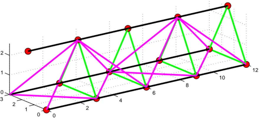
In recent years there has been renewed interest in Rigidizable-Inflatable (RI) space structures because of the efficiency they offer in packaging during boost-to-orbit. RI materials offer the possibility of deploying large space structures ([7]) and so are of interest in applications where large optical or RF apertures are needed. Several proposed space antenna systems will require ultra-light trusses to provide the “backbone” of the structure (see Figure 1(a)). It has been widely recognized that practical precision requirements can only be achieved through the development of new high-fidelity mathematical models and corresponding numerical tools.
In this paper we study the dynamics of a basic truss component consisting of two RI beams connected through a joint (see Figure 1(b)). One of the more im-portant characteristics of such space systems is their response to changing thermal loads, as they move in and out of the Earth’s shadow. In this paper we study the thermoelastic behavior of a two-beam truss element subject to solar heating. The beams are fabricated as thin-walled circular cylinders.
Key words and phrases. Truss structures, Euler-Bernoulli beams, thermoelastic system.
0
2
4
6
8
10
12
0 1 2 3 0 1 2
(a) Rigidizable-Inflatable truss structure
Joint
x
y
Beam−1
Beam−2
φ1
φ2
Leg 1
Leg 2
s1=0
s1=L1 s2=L2
s2=0
w1(t,s 1)
w2(t,s 2)
(b) Basic structure of the joint-legs-beams system
Figure 1.1. Truss (a) and basic structure of the joint-legs-beams
system (b).
2. Thermoelastic Model
The equations of motion for the Joint-Leg-Beam system depicted in Figure 1(b) are the following (see [1] for details):
ρiAi
∂2ui(t, si)
∂t2 =EiAi
∂2ui(t, si)
∂s2
i
, ρiAi
∂2wi(t, si)
∂t2 =−EiIi
∂4wi(t, si)
∂s4
i
Md
2 dt
x(t)y(t)θ1(t)θ2(t)
T =C
M1(t)N1(t)M2(t)N2(t)F1(t)F2(t)
T (2.2)
for timet >0 and spatial variablesi∈[0, Li], whereM andCare 4×4 and 4×6 matrices give by
M=
2
6 6 4
m 0 −m1d1cosϕ1 m2d2cosϕ2
0 m m1d1sinϕ1 m2d2sinϕ2
−m1d1cosϕ1 m1d1sinϕ1 I1ℓ+m1d 2
1 0
m2d2cosϕ2 m2d2sinϕ2 0 I2ℓ+m2d
2 2
3
7 7 5
, (2.3)
C=
2
6 6 4
0 −cosϕ1 0 cosϕ2 sinϕ1 sinϕ2 0 sinϕ1 0 sinϕ2 cosϕ1 −cosϕ2
1 ℓ1 0 0 0 0
0 0 1 ℓ2 0 0
3
7 7 5
, (2.4)
and the other functions and parameters are as follows (here the supra or sub-index
i, i = 1,2 will always refer to beam or leg i): ui(t, si), wi(t, si) longitudinal and transversal displacement of the beam; x(t), y(t) horizontal and vertical displace-ment of the joint’s tip; θi(t) rotation angle of the leg; ρi, Ai, Li, Ei, Ii mass den-sity, cross section area, length, Young’s modulus, moment of inertia of the beam;
mi, di, ℓi, Iℓi mass, center of mass, length, moment of inertia of the leg; mp mass of the joint,m=m1+m2+mp; ϕ1 initial angle of leg 1 with positivey axis;ϕ2
initial angle of leg 2 with negative y axis; Fi(t) extensional force of beam at the endsi=Li;Ni(t) shear force of beam at the endsi=Li;Mi(t) bending moment of beam at the endsi=Li.
Each beam is clamped at the end si = 0. Thus the boundary conditions at
si= 0 are
ui(t,0) =wi(t,0) = ∂w i
∂si
(t,0) = 0, i= 1,2. (2.5)
At the other end of each beam several obvious geometric compatibility conditions must be imposed. These conditions can be written in the form:
− ∂ ∂s1w
1(t, L 1) w1(t, L1) − ∂
∂s2w 2(t, L
2) w2(t, L
2) −u1(t, L
1) −u2(t, L
2)
=
θ1(t)
−x(t) cosϕ1+y(t) sinϕ1+ℓ1θ1(t) θ2(t)
x(t) cosϕ2+y(t) sinϕ2+ℓ2θ2(t) x(t) sinϕ1+y(t) cosϕ1 x(t) sinϕ2−y(t) cosϕ2
=CT
x(t)
y(t)
θ1(t) θ2(t)
.
3. Thermal Dynamics
The external heat flux in the space normal to the beam’s surface is given by (see [10])
Si=. S0 cos
ξi−
∂wi
∂si
, (3.1)
where S0 denotes the solar flux andξi the angle of orientation of the solar vector with respect to the beam. In this equation we shall neglect the contribution of
∂wi
∂si since we are assuming it is small. We denote by T i(t, s
i, φi) the deviation of the temperature of the thin-walled circular beami with respect to a reference temperatureTi
0at timetat the point on the beam corresponding to axial coordinate si and circumferential coordinate φi (here φi = 0 corresponds to the top of the beam whileφi=πcorresponds to the bottom). Conservation of energy for a small segment of circular cylinder including longitudinal and circumferential conduction in the cylinder wall and radiation from the cylinder’s surface yields the following equation forTi:
ρici∂T i
∂t − ki
c
R2
i
∂2Ti
∂φ2
i
−kai
∂2Ti
∂s2
i +σǫi
hi
(T0i+Ti)4= αi
s
hi
Sicos(φi)δ(φi) (3.2)
whereki
a andkci are the axial and circumferential thermal conductivity coefficients, respectively,ci is the specific heat,Rithe radius of the cylinder,hiis the thickness of the wall,ǫi is the surface emissivity andαis is the surface absorptivity,σ is the Stefan-Boltzmann constant, δ is a function defined on [−π, π] by δ(φi) = 1 for
φi∈(−π2,π2), andδ(φi) = 0 forφi ∈[−π,−π2]∪[π2, π]. The heat flux distribution on the RHS of equation (3.2) can be written as
Si cos(φi)δ(φi) = Si 1
π+g(φi)
= Si
π +Sig(φi) (3.3)
whereg(φi)= cos(. φi)χ
[−π2, π2]
(φi)−1π (hereχdenotes the characteristic function). Clearlyg(φi) is continuous and it has zero average in [−π, π].
For each beam, the temperature distribution is separated into two parts, namely:
Ti(t, s
i, φi) =Ti(t, si) +Tm,i(t, si)g(φi), (3.4)
where Ti(t, si) is independent of φ
i and corresponds to the uniform part of the flux, Si
π, in (3.3), and T
m,i(t, si)g(φi) amounts for the circumferential variation
of the flux in (3.3). Note that for every si ∈ [0, Li] and t ≥ 0 one has that
Tm,i(t, si) =Ti(t, s
i,0)−Ti(t, si, π) = Ti(t, si,0)−Ti(t, si, φ) for anyφ /∈[−π2,π2]. Hence,Tm,i(t, si) can be thought of as the thermal gradient between the top and the bottom of the beam at the axial locationsi.
Also, we approximate the thermal radiation term (Ti
0+Ti(t, si, φi) )4in (3.2) by linearizing T(t, si, φi) around T(t, si, φi) =Tsi (whereTsi, to be determined later, is the steady-state constant temperature increment produced on the undeformed beamiby the solar fluxSi), i.e., we approximate (Ti
4(Ti
0+Tsi)3 Ti(t, si)−Tsi+Tm,i(t, si)g(φi)
. Hence equation (3.2) is replaced by
ρici∂T i(t, si)
∂t +ρici
∂Tm,i(t, si)
∂t g(φi)− ki
c
R2
i
Tm,i(t, si)g′′(φi)
−kia
∂2Ti(t, si)
∂s2
i
−kia
∂2Tm,i(t, si)
∂s2
i
g(φi)
+σǫi
hi
(T0i+Tsi)4+ 4(T0i+Tsi)3 Ti(t, si)−Tsi+Tm,i(t, si)g(φi)
=α i sSi
hi 1
π+g(φi)
. (3.5)
Since g has zero average, integration of equation (3.5) over the cylinder’s cross sectional area yields
ρici
∂Ti(t, si)
∂t −k
i a
∂2Ti(t, si)
∂s2
i
+4σǫi(T i
0+Tsi)3
hi
[Ti(t, si)−Ti s]
= αi
sSi
πhi
−σǫi(T
i
0+Tsi)4
hi
.
=fi. (3.6)
Sinceg′(φ
i) is discontinuous atφi =±π2 the integration ofg′′(φi) above must be performed in the distributional sense. The value ofTi
sis now determined by setting the RHS,fi, equals to zero. By doing so we obtain
Ti s=
αi sSi
πσǫi 14
−Ti
0 (3.7)
Note that with this value ofTi
scorresponds to the steady-stateTi(t, si) =Tsifor the case of homogeneous Neumann boundary conditions and, since usuallyTm,i(t, s
i) is small compared toTi
0, the linearization of the thermal radiation term performed
above, is justified near the steady state solution.
Now multiplying (3.5) byg(φi) and integrating over the cylinder’s cross sectional area, we obtain forTm,i the following equation:
ρici
∂Tm,i(t, si)
∂t −k
i a
∂2Tm,i(t, si)
∂s2
i
+
ki cπ2
R2
i(π2−4)
+4σǫi(T i
0+Tsi)3
hi
Tm,i(t, si) = α i sSi
hi
.
(3.8)
Thermally induced vibrations in the system is taken into account by considering Hooke’s law for the stress-strain relation in the formǫi
11=E1iσ i
11+αiTi,whereαi is the thermal expansion coefficient, andTi is, as before, the deviation from the reference temperature Ti
0. Note that atTi = 0 thermal strain vanishes, so that Ti
0 is interpreted as the (uniform) temperature of beam i in the unstressed,
rest-state. By the standard derivation of Euler-Bernoulli beam equation, we modify the Joint-Leg-Beam system (2.1) as follows:
ρiAi
∂2ui(t, si)
∂t2 = EiAi ∂ ∂si
∂ui(t, si)
∂si
−αiTi(t, si)
ρiAi
∂2wi(t, si)
∂t2 = −EiIi ∂2 ∂s2
i
∂2wi(t, si)
∂s2
i
+ αi 2RiT
m,i(t, s i)
(3.10)
The above beam equations are coupled to the heat equations modified from equa-tions (3.6) and (3.8) and with Ti
s chosen as in equation (3.7) (so that fi = 0 in (3.6) ), that is:
ρici
∂Ti(t, si)
∂t =k
i a
∂2Ti(t, si)
∂s2
i
−4σǫi(T
i
0+Tsi)3
hi
Ti(t, si)−Tsi
−αiEiT0i ∂2 ∂si∂t
ui(t, si),
(3.11)
and
ρici
∂Tm,i(t, si)
∂t =k
i a
∂2Tm,i(t, si)
∂s2
i
−
ki cπ2
R2
i(π2−4)
+4σǫi(T i
0+Tsi)3
hi
Tm,i(t, si)
+αiEiIiT i
0
2RiAi
∂3 ∂s2
i∂t
wi(t, si) +
αi sSi
hi , (3.12)
We impose Robin type boundary conditions for the temperature at both ends of each beam, i.e.
∂ ∂si
Ti(t, L
i, φi) =λiR `
T∗
−T0i−Ti(t, Li, φi)´,
∂ ∂si
Ti(t,0, φ i) =λiL
`
Ti
0+Ti(t,0, φi)−T∗ ´
,
∀t ≥0, φi ∈[−π, π], i= 1,2, where T∗ is the temperature of the surrounding medium andλi
L,λiR,i= 1,2, are nonnegative constants. By writingTi(t, si, φi) in terms of the decomposition given in (3.4) these equations take the form:
∂ ∂si
Ti(t, Li) + ∂
∂si
Tm,i(t, Li)g(φi) =λiR T∗−T0i−Ti(t, Li)−Tm,i(t, Li)g(φi)
,
∂ ∂si
Ti(t,0) + ∂
∂si
Tm,i(t,0)g(φi) =λiL T0i+Ti(t,0) +Tm,i(t,0)g(φi)−T∗
.
Since these equations must hold for allφi∈[−π, π] it follows that
∂ ∂si
Ti(t, Li) =λiR T∗−T0i−Ti(t, Li)
, ∂
∂si
Ti(t,0) =λiL T0i+Ti(t,0)−T∗
(3.13)
and
∂ ∂si
Tm,i(t, Li) =−λi
RTm,i(t, Li),
∂ ∂si
Tm,i(t,0) =λi
LTm,i(t,0), (3.14)
for all t ≥ 0, i = 1,2. So, in the same way that the dynamics for the tem-perature distribution (3.5) decouples into equations (3.11) and (3.12) for Ti and
Ti(t, si)−(T∗−Ti
0), equation (3.11) can be written in the form ρici∂
˜
Ti(t, si)
∂t =k
i a
∂2T˜i(t, si)
∂s2
i
−4σǫi(T
i
0+Tsi)3
hi
˜
Ti(t, si) +T∗−Ti
0−Tsi
−αiEiT0i ∂2 ∂si∂tu
i(t, si),
(3.15)
while the boundary conditions (3.13) now take the form
∂ ∂si
˜
Ti(t, Li) =−λi
RT˜i(t, Li),
∂ ∂si
˜
Ti(t,0) =λi
LT˜i(t,0), (3.16)
Observe now that these boundary conditions are exactly the same as those in (3.14) for the circumferential component of the temperature. Finally, note also that in equation (3.9),Ti(t, si) can be replaced by ˜Ti(t, si) without any changes.
System (3.9)-(3.12) (or equivalently (3.9), (3.10), (3.12), (3.15)), together with the joint-leg dynamics described by equation (2.2) constitute the thermoelastic Joint-Leg-Beam equations with the external solar heat source. The extensional forces, shear forces and bending moments of the beams atsi =Li are now given by:
Fi(t) = EiAi
∂ui
∂si
(t, si)−αiTi(t, si)
s
i=Li
, (3.17)
Ni(t) = EiIi ∂
∂si
∂2wi
∂s2
i
(t, si) + αi 2Ri
Tm,i(t, si)
s
i=Li
, (3.18)
Mi(t) = EiIi
∂2wi
∂s2
i
(t, si) + αi 2Ri
Tm,i(t, si)
si=Li
. (3.19)
4. Well-posedness
In this section, we consider the well-posedness of the Joint-Leg-Beam system with solar heat flux, i.e., equations (3.9), (3.10), (3.12), (3.15) subject to the geo-metric beam-leg interface compatibility conditions (2.6), the dynamic boundary conditions (3.17), (3.18), (3.19) and the boundary conditions (2.5), (3.14), (3.16). We first rewrite the system as a first order evolution equation in an appropriate Hilbert space. Well-posedness is then obtained by using semigroup theory. Since the corresponding system without thermal effects has been studied in [1], we will follow the notation used there as much as possible for consistency. Numerical results for that case are reported in [2].
First, we define the following Hilbert spaces with their corresponding inner prod-ucts:
Hz=L2(0, L1)×L2(0, L2)×L2(0, L1)×L2(0, L2), hz1, z2iHz
.
=
2
X
i=1
ρiAihwi1, w2ii+hui1, ui2i
Hb= [ker(C)]⊥= range(CT),
hb1, b2iHb=hb1,(C
TM−1C)†b
2ilR6;
Hζ =L2(0, L1)×L2(0, L2)×L2(0, L1)×L2(0, L2), hζ1, ζ2iHζ
.
=
2
X
i=1 ρiciAi
Ti
0
h
hT1m,i, T2m,ii+hT˜1i,T˜2ii
i ;
where zj =. w1j, w2j, u1j, u2j T
, ζj =.
Tjm,1, Tjm,2,T˜1
j,T˜j2 T
, and (CTM−1C)†
denotes the Moore-Penrose generalized inverse of CTM−1C. We also define the
operatorsAz:Hz→ Hz andBz:Hζ → Hz by
dom(Az) =. Hℓ2∩H4(0, L1)×Hℓ2∩H4(0, L2)×Hℓ1∩H2(0, L1)×Hℓ1∩H2(0, L2),
Az =.
E1I1
ρ1A1D
4 0 0 0
0 E2I2
ρ2A2D
4 0 0
0 0 −E1
ρ1 D
2 0
0 0 0 −E2
ρ2 D 2 ,
dom(Bz) =. H2(0, L1)×H2(0, L2)×H1(0, L1)×H1(0, L2),
Bz =.
−α1E1I1 2R1ρ1A1D
2 0 0 0
0 − α2E2I2 2R2ρ2A2D
2 0 0
0 0 −α1E1
ρ1 D 0
0 0 0 −α2E2
ρ2 D
.
whereDn=. dn dsn
i and forn∈IN,H n
ℓ(0, L) denotes the space of functions inHn(0, L) that vanish, together with all derivatives up to the ordern−1, at the left boundary. With this notation, equations (3.9)-(3.10) can now be written as the following abstract second order ODE inHz:
¨
z(t) +Azz(t)− Bzζ(t) = 0. (4.1)
Next we define the operatorsAζ :Hζ → Hζ andBζ :Hz→ Hζ by
dom(Aζ)=. Hrb2(0, L1)×Hrb2(0, L2)×Hrb2(0, L1)×Hrb2(0, L2),
Aζζ=Aζ
Tm,1 Tm,2
˜ T1 ˜ T2 . =
− k1a ρ1c1D
2Tm,1+h k1cπ 2
ρ1c1R21(π2−4)+
4σǫ1(T01+T 1 s)
3
ρ1c1h1
i
Tm,1 − k2a
ρ2c2D
2Tm,2+h k2cπ 2
ρ2c2R22(π2−4)+
4σǫ2(T02+T 2 s)
3
ρ2c2h2
i
Tm,2 − k1a
ρ1c1D
2T˜1+4σǫ1(T01+Ts1) 3
ρ1c1h1
˜
T1 − k2a
ρ2c2D
2T˜2+4σǫ2(T02+Ts2) 3
ρ2c2h2
˜ T2 ,
Bζz=.
α1E1I1T01 2R1ρ1c1A1D
2 0 0 0
0 α2E2I2T02 2R2ρ2c2A2 D
2 0 0
0 0 −α1E1T01
ρ1c1 D 0
0 0 0 −α2E2T02
ρ2c2 D
.
where H2
rb(0, L) denotes the space of functions in H2(0, L) satisfying the Robin boundary conditions (3.14) or equivalently (3.16). With this notation, equations (3.12), (3.15), can now be written as the following abstract first order ODE inHζ:
˙
ζ(t)− Bζz˙(t) +Aζζ(t) = S (4.2)
where
S=. α1s ρ1c1h1S1,
α2s ρ2c2h2S2,
4σǫ1 (T0 +1 Ts1)3 ρ1c1h1 (T
1
s+T01−T∗),
4σǫ2 (T0 +2 Ts2)3 ρ2c2h2 (T
2
s+T02−T∗)
T
.
We also define three boundary projection operatorsPB
1 ,P2B fromHz into IR6and
PB
3 from Hζ into IR6 by dom(PB
1 ) .
= H2(0, L
1)×H2(0, L2)×H1(0, L1)×H1(0, L2),
dom(PB
2 ) =. H4(0, L1)×H4(0, L2)×H2(0, L1)×H2(0, L2),
dom(P3B) =. H2(0, L1)×H2(0, L2)×H1(0, L1)×H1(0, L2),
P1B 0 B B @ w1 w2 u1 u2 1 C C A . = 0 B B B B B B @ − ∂
∂s1w 1
(L1)
w1(L1)
− ∂
∂s2w 2
(L2)
w2(L2)
−u1(L1)
−u2(L2) 1 C C C C C C A
, P2B 0 B B @ w1 w2 u1 u2 1 C C A . = 0 B B B B B B B B B B B B @ ∂2 ∂s2 1
w1(L 1) ∂3 ∂s3 1
w1(L 1) ∂2 ∂s2 2
w2(L 2) ∂3 ∂s32w
2(L 2) ∂ ∂s1u
1(L 1) ∂ ∂s2u2(L2)
1 C C C C C C C C C C C C A
, P3B 0
B B @
Tm,1
Tm,2 ˜ T1 ˜ T2 1 C C A . = 0 B B B B B B B @
Tm,1(L 1) ∂ ∂s1T
m,1(L 1)
Tm,2(L 2) ∂ ∂s2T
m,2(L 2) ˜
T1(L 1) ˜
T2(L 2) 1 C C C C C C C A .
Now, by using the geometric compatibility conditions (2.6) and the dynamic boundary conditions (3.17)-(3.19), the equation for the leg-joint dynamics (2.2) can be written as the following abstract second order ODE inHb:
d2 dt2 P
B
1 z(t)
−CTM−1CE PB
2 z(t) + ΛP3Bζ(t)
= ˜R (4.3)
whereE=. diag(E1I1, E1I1, E2I2, E2I2, E1A1, E2A2), Λ= diag(. 2αR11,2αR11,2αR22,2αR22, −α1,−α2) and ˜R=. CTM−1C 0, 0, 0, 0, E1A1α1(T∗−T01), E2A2α2(T∗−T02)
T . Next we define the Hilbert spaceHzb =. Hz×Hbwith the usual inner product inher-ited from those inHz andHb. In this Hilbert space we define the elastic operator
Azb by
dom(Azb)=.
z b
∈dom(Az)× Hb : P1Bz=b
andAzb z b . =
Azz
−CTM−1CE PB
2 z
Furthermore, we defineBzb:Hζ → Hzb by dom(Bzb) =. H2(0, L1)×H2(0, L2)× H1(0, L
1)×H1(0, L2) and Bzbζ =.
Bzζ
CTM−1CEΛPB
3 ζ
. Thus, equations (4.1)
and (4.3) can be combined as
d2 dt2
z(t)
b(t)
+Azb
z(t)
b(t)
− Bzbζ(t) = R onHzb, (4.4)
where R= (0. ,R˜)T. It has been proved in [1] that the operatorA
zb is self-adjoint and strictly positive. Thus, we can define the state space H = dom(. A1zb/2)× Hzb× Hζ with the inner product
* X
1
X2
X3
!
,
Y1
Y2
Y3
!+
H
.
= hA1zb/2X1,Azb1/2Y1iHzb + hX2, Y2iHzb +hX3, Y3iHζ. Finally, we define operator A on H by dom(A)
.
=
X1 X2 X3
∈ H
X1∈dom(Azb), X2∈dom(Azb1/2), X3∈dom(Aζ)
, A
X1
X2
X3
!
.
=
0 I 0
−Azb 0 Bzb
0 (Bζ,0) −Aζ ! X
1
X2
X3
!
. Then, equations (4.2) and (4.4) can be rewritten
as a first order nonhomogeneous evolution equation ˙
X(t) =AX(t) +G on H (4.5)
whereX =.
X1 X2 X3
, X1=.
z b
, X2= ˙. X1, X3=. ζ and G=.
0
R S
.
Theorem 4.1. (Well-posedness): Let A:H → H be as defined above. ThenAis
the infinitesimal generator of a strongly continuous semigroup of contractionsS(t)
on Hand hence, for any initial conditionX0=X(0)∈dom(A), system(4.5)has a unique global solutionX(t)given by
X(t) =S(t)X0+
Z t
0
S(t−s)G ds.
Proof: It can be shown that A is dissipative and 0 ∈ ρ(A), the resolvent set of A). Since dom(A) is dense in H, it then follows from Theorem 1.2.4 in [8] that Agenerates a strongly continuous semigroup of contractionsS(t) onH. The existence and uniqueness of solutions for system (4.5) for any initial condition
X0 =X(0)∈dom(A) finally follows from Corollary 2.10 in [9]. For more details
see [3].
5. Exponential Stability
type of system is often referred to as “hybrid system”. It is certainly an interest-ing problem to determine whether the thermal dampinterest-ing is strong enough by itself to induce exponential stability of this kind of system. We shall prove this in the affirmative.
The following result by Huang [6] will be used:
Theorem 5.1. Let H be a Hilbert space, A : H → H a closed, densely defined
linear operator. Assume thatA generates a C0-semigroup of contractions T(t)on H. Then T(t)is exponentially stable if and only if
ilR∩σ(A) =∅, (5.1)
lim β→∞k(
iβ−A)−1k<∞. (5.2)
Theorem 5.2. TheC0-semigroup of contractions S(t) generated byA(see
Theo-rem 4.1) is exponentially stable.
Proof: If (5.2) is false then there exists a sequence{βn} ⊂lR withβn→ ∞ and a sequence{Xn} ⊂D(A) withkXnkH= 1∀nsuch that
lim n→∞k(
iβn− A)XnkH= 0. (5.3)
Using the components related to the thermoelastic beam equations it can be show that (5.3) yields the contradictionkXnkH→0 asn→ ∞. Similarly, if the condition
(5.1) is false, then there existβ∈lR and a sequence{Xn} ⊂D(A) withkXnkH=
1 ∀n, such that
lim n→∞k(
iβ− A)XnkH= 0. (5.4)
By repeating the same arguments we get the contradiction kXnkH → 0. For
complete details on these proofs, we refer the reader to [3]. Hence A satisfies conditions (5.1) and (5.2) and therefore, the C0-semigroup of contractions S(t)
generated byAis exponentially stable.
6. Conclusions
In this article we considered a system of two thermoelastic Euler-Bernoulli beams coupled to a joint through two legs. By means of semigroup theory the well posed-ness of the system was proved and its exponential stability was derived. It is certainly of much interest to develop numerical approximations for our state-space model (4.5). Such numerical schemes will be useful in simulation and identification studies to predict and better understand the structural and thermal responses of space-borne observation systems. Efforts in this direction are already under way.
Acknowledgements
References
[1] J.A. Burns, E.M. Cliff, Z. Liu and R. D. Spies, On Coupled Transversal and Axial Motions of Two Beams with a Joint, Journal of Mathematical Analysis and Applications, Vol. 339, 2008, pp 182-196.
[2] J.A. Burns, E.M. Cliff, Z. Liu and R. D. Spies, Results on Transversal and Axial Motions of a System of Two Beams coupled to a Joint through Two Legs, submitted, 2008. ICAM Report 20070213-1.
[3] E.M. Cliff, B. Fulton, T. Herdman, Z. Liu and R. D. Spies, Well posedness and exponential stability of a thermoelastic joint-leg-beam system with Robin boundary conditions, Mathemat-ical and Computer Modelling (2008), en prensa, DOI: 10.1016/j.mcm.2008.03.018.
[4] J.A. Burns, E.M. Cliff, Z. Liu and R. D. Spies, Polynomial stability of a joint-leg-beam system with local damping, Mathematical and Computer Modelling, Vol. 46, 2007, pp 1236-1246. [5] J.A. Burns, Z. Liu and S. Zheng, On the Energy Decay of a Linear Thermoelastic Bar. J. of
Math. Anal. Appl., Vol. 179, No. 2, 1993, pp 574-591.
[6] F. L. Huang,Characteristic Condition for Exponential Stability of Linear Dynamical Systems in Hilbert Spaces, Ann. of Diff. Eqs., 1(1), 1985, pp 43-56.
[7] C. H. M. Jenkins (ed.), Gossamer Spacecraft: Membrane and Inflatable Technology for Space Applications, AIAA Progress in Aeronautics and Astronautics, (191), 2001.
[8] Z. Liu and S. Zheng,Semigroups Associated with Dissipative Systems, 398 Research Notes in Mathematics, Chapman & Hall/CRC, 1999.
[9] A. Pazy, Semigroups of Linear Operators and Applications to Partial Differential Equations, Second Edition, Springer Verlag, 1983.
[10] E. A. Thornton and R. S. Foster,Dynamic Response of Rapidly Heated Space Structures. In: Computational Nonlinear Mechanics in Aerospace Engineering, edited by Atluri, S.N., Progress in Astronautics and Aeronautics, Vol. 146, AIAA, Washington D.C., 1992, p. 451-477.
E. M. Cliff
Interdisciplinary Center for Applied Mathematics Virginia Polytechnic Institute and State University Blacksburg, VA, 24061-0531, USA.
Z. Liu
Department of Mathematics University of Minnesota Duluth, MN 55812-3000, USA.
R. D. Spies
Instituto de Matem´atica Aplicada del Litoral IMAL, CONICET-UNL, G¨uemes 3450, and Departamento de Matem´atica,
Facultad de Ingenier´ıa Qu´ımica, UNL, Santa Fe, Argentina
rspies@imalpde.santafe-conicet.gov.ar