Competition Policy for Elections: Do Campaign Contribution Limits Matter?
Thomas Stratmann Department of Economics George Mason University
Francisco J. Aparicio -Castillo Political Studies Division
CIDE, Mexico
Abstract
This paper examines whether campaign contribution restrictions have consequences for election outcomes. States are a natural laboratory to examine this issue. We analyze elections to Assemblies from 1980 to 2001 and determine whether candidates’ vote shares are altered by changes in state campaign contribution restrictions. We find that limits on giving narrow the margin of victory of the winning candidate. Limits lead to closer elections for future incumbents, but have less effect on the margin of victory of incumbents who passed the campaign finance legislation. We also find some evidence that contribution limits increase the number of candidates in the race.
I. Introduction
Campaign finance reform is a vigorously debated issue in virtually every U.S. election, both congressional and presidential. Some claim large amounts of campaign spending turn political races into fund-raising contests biased in favor of incumbents, while others argue that unrestricted spending may be the only way for challengers to even the playing field. To date, scant evidence exists regarding the effects of campaign finance restrictions on election outcomes. Whether stricter regulations amount to incumbency protection laws, or whether they help challengers to compete remain an unanswered empirical question.
A number of theoretical models emphasize the fact that campaign contributions are used in electoral races to provide information to voters (see for example Austin-Smith 1987, Pooters, Sloof, and van Winden 1997, Coate 2001, 2002, Prat 2002a, 2002b). However, little is known about the empirical validity of these models, a fact echoed in the public debate over campaign finance reform. U.S. Senator Mitch McConnell (R-Kentucky), for example, claims that most contribution limits proposals amount to “incumbent protection acts,” and commissioner Bradley A. Smith of the Federal Election Commission argues that “campaign finance laws also tend to favor incumbents by making it harder for challengers to raise money vis -à-vis incumbents” (Smith 1995). Those who favor stricter contribution limits claim that limits “level the playing field.” Some advocates favor limiting contributions because if limits were increased, “higher limits would increase the disparity in challenger-incumbent fundraising.”1
The academic debate regarding campaign spending’s effect on vote shares goes back to Jacobson’s (1978) groundbreaking study on the issue. Since his initial work, many scholars have analyzed this relationship. The more recent literature on campaign spending finds a positive effect of challenger campaign spending on challengers’ vote shares and a sometimes smaller, but still positive effect for incumbent spending on incumbents’ vote shares (Grier 1989, Green and Krasno 1988). Though some limited inferences regarding contribution limits can be drawn from these studies, they do not directly address the electoral consequences of campaign finance regulation. Because these studies took place at the federal level, where federal campaign finance laws had not changed since the mid-1970s, they offer little insight into this issue. As a result, we can derive very little from the previous data analyses regarding the effects of campaign finance rules on political outcomes.2
Although federal campaign finance laws have changed very little until the recent 2002 legislation (BICRA), state campaign finance laws exhibit sufficient variation across states and over time. Since the
1
We obtained this quote from a publication by the Public Interest Research Group, http://pirg.org/democracy/ (accessed August 2, 2002).
2
late1970s, many states have enacted and changed their own campaign finance laws. Thus, state-level regulations implemented over the past twenty years have the potential to provide insight into the effects of campaign finance regulation on vote shares and the closeness of elections, and also provide a natural testing ground for theoretical campaign finance models.
Some previous studies examine state campaign finance rules but tend to be limited in scope (Malbin and Gais 1998, Thompson and Moncrief 1998).3 The current paper represents the first systematic study that comprehensively examines the effects of state-level campaign finance regulation over the past twenty years. This study treats each of the states with single member districts as campaign finance reform laboratories. It examines the effects of these laws, enacted in the 1980s and 1990s, and uses the margin of victory and the number of candidates as outcomes of the political process.
Our statistical analysis shows that after controlling properly for other factors that may determine election outcomes, limits on contributions lead to closer elections. Both, introducing limits and tightening existing limits increases the closeness of elections.4 Moreover, we find that the introduction of
contribution limit restrictions impacts future incumbents more than it impacts incumbents who passed the contribution law. Finally, we examine the effect of contribution limits on the number of candidates and show that tighter limits are associated with an increase in the number of candidates in a given district.
Section II presents theoretical examples that illustrate the ambiguous effect of campaign finance limits on the competitiveness of elections. We present the empirical model in section III, discuss some
3
Malbin and Gais (1998), describes and evaluates state reforms between 1980 and 1996, and Thompson and Moncrief (1998) studies a sample of 18 states. Other scholars (Kettl et al. 1997, Mayer 1998, Redfield 1995, 2000) have studied individual states in detail. Examining a 1994 cross-section of states, Hogan (2000) shows a correlation between state contribution limits and legislative campaign expenditures, but its impact on electoral outcomes is not addressed. Hogan (2000) shows that stricter contribution laws correlate with significantly lower campaign spending, primarily by incumbents. Kousser and LaRaja (2000) study contribution laws and fundraising patterns in a sample of legislative races in 1996. Using gubernatorial elections, Gross, Goidel, and Shields (2002) study campaign finance regulations and campaign spending, and Milyo, Primo, and Groseclose (2002) study contribution limits, turnout, and partisan advantage.
4
data issues in section IV, provide the estimation results in section V, discuss the underlying mechanism in section VI, and conclude in section VII.
II. Theoretical Framework
Scholars who have examined the effectiveness of campaign spending in elections have formed a number of hypotheses regarding the effect of contribution limits on election outcomes. Jacobson (1978), for example, suggests that challengers would be mostly hurt by contribution limits because his estimates suggest that the productivity of challenger spending is significantly larger than the productivity of
incumbent spending. In contrast, Green and Krasno’s (1988) finding that incumbents’ and challengers’ campaign spending has an equal marginal impact on their respective vote shares, suggests that
contribution limits have an equal impact on incumbents and challengers.
In most recent formal models of candidate competition with campaign expenditures, campaign advertisements inform voters about candidates’ positions. Campaign expenditures increase the precision with which voters estimate the position of candidates (Austen-Smith 1987), inform voters about the candidate quality (Ortuno -Ortin and Schultz 2000, and Coate 2001, Wittman 2002), or provide a signal about candidate quality (Potters, Sloof, and van Winden 1997, Prat 2002). Most of these models imply that limiting or banning contributions reduces the information about candidates’ positions or quality. Candidates differ in their quality, and if contributions are only position induced, then some of these models suggest that the absence of campaign expenditures reduces the probability that a voter casts a ballot for the high quality candidate, resulting in closer electoral margins.
Coate (2002) specifically addresses the issue of limiting contributions. He shows under which conditions limits on contributions increase or decrease the margin of victory of the winning candidate. This model provides the testable implication that campaign contribution limits effect the closeness of elections. If contributions are only position induced, then contribution limits lead to a narrowing of the margin of victory. However, if contributions are also service induced (i.e. there is a quid pro quo), then limits on contributions can increase the margin of victory. In the latter case, limits reduce the amount of favors promised and thus voters find the campaign message of high quality candidates more credible, leading to an increase of their margin of victory.5
Early models on campaign financing suggest that incumbents have an advantage through brand name recognition, which is a function of current campaign spending and campaign spending in previous elections. However, these models are not grounded in formal models that fully describe the attributes of contributors, voters, and candidates. They generate the prediction that limits lead to closer elections, because contribution limits curtail an incumbent’s ability to accumulate a brand name.6 Contribution limits lead to less brand name development by incumbents and give challengers a competitive
5
In Coate’s (2002) model voters believe that even high quality candidates promise favors to contributors, and thus voters become cynical. With unrestricted contributions and unrestricted favor selling (candidates are infinitely power hungry), the informational value of contributions becomes very small. Therefore, contribution limits can increase the effectiveness of the high quality candidate’s campaign spending by increasing his vote share.
6
advantage.7 Curtailing contributions helps challengers relative to incumbents, and limits reduce the amount that incumbents outspent challengers. Although incumbents still have an advantage relative to challengers, limiting contributions reduces, but does not eliminate, the incumbents' competitive advantage. The brand name model also has implications for challenger entry. If contribution limits effectively raise the competitive advantage of challengers, more challengers will enter the race when limits are in place. This model predicts that legislators who become incumbents after the implementation of contribution limits receive lower vote shares than legislators who accumulated a brand name prior to contribution limits.
III. Research Design and Methods
To analyze the effect of campaign finance laws on electoral outcomes, we use the state Assembly single member district as the unit of analysis. We estimate the regressions
Yijt = ßCFLAWit + Xijt ? + µi + vt + eijt , (1)
Yijt = ßCFLAWit + Xijt ? + dij + vt+ eijt , (2)
where Yijt is the electoral outcome measured either as closeness of the election in state i, district j, and election year t, or as the number of candidates in the race. The regressions differ in that the first specification includes state fixed effects (µi) and the second specification includes district fixed effects (dij). We control for changes in national laws and national events that affect local elections via year fixed effects vt. We estimate regressions (1) and (2) for two samples. One sample includes races involving incumbents only, and another sample includes all races. In most specifications we adjust the standard errors for non-independence of the observations within state-years.
In the simplest specification CFLAW is an indicator variable, which equals one when the campaign finance law restricts contributions in state Assembly elections, and zero otherwise. The coefficient on the CFLAW indicator is identified by states that changed their law from allowing unlimited contributions to limited contributions and vice versa. In an alternative specification, CFLAW is the real contribution limit amount for state Assembly races in states that have adopted contribution restrictions.
Restrictions on contributions come in various forms as states have adopted limits on
contributions for individuals, Political Action Committees (PACs), corporations, unions, and parties. We created an indicator for whether contributions are restricted from each of these five sources. We will analyze the impact of these restrictions by creating an index that measures how many sources of contributions were subject to a limit. This index is the sum of these five indicators, and thus the index ranges between zero and five.
The Xijtvector includes candidate and district specific variables and ? is the corresponding vector of coefficients. The X vector includes variables such as whether or not the particular race is an open seat election, whether or not the incumbent was in office when the law was changed, the previous margin of victory of the incumbent, and the number of candidates in the district. As mentioned
7
previously, we control for time-invariant state characteristics with state fixed effects or alternatively district fixed effects. State fixed effects capture differences across states that may influence the
competitiveness of state elections such as the professionalism of legislatures and legislator salaries. State indicators also capture the fact that their populations and actual sizes differ greatly, which in part
explains differences in campaign spending across states (Gierzynski and Breaux 1991, Hogan 2000) and differences in campaign technology. Lastly, state effects control for omitted time -invariant state characteristics that simultaneously determine vote shares and campaign finance regulations. District fixed effects capture everything that is captured by state effects, as well as district level variables that are constant over time such as whether the district is urban or rural.
One potential concern with the analysis is whether or not the passage and modification of state campaign finance laws represent a natural experiment. A natural experiment is an exogenous source of variation that determines the treatment assignment. Electoral races in states after the passage of
campaign finance laws constitute the treatment groups, while races in states without such laws and races in states prior to the implementation of the laws constitute the comparison groups.
The implementation of the law is not random, however, given that legislators decid e what kind of law to pass, which will affect them in the next election campaign. Furthermore, contribution laws respond to voters’ concerns regarding spending levels, which also influence election outcomes. In the 1990s, for example, some campaign finance laws tightened through voter initiatives. Thus, the campaign finance law variable may be endogenous in the vote share equation. If stricter limits help challengers, incumbents would loosen restrictions in the face of more competitive elections, leading to an
underestimation of the effect of contribution laws on election closeness.8 Also, the contribution limit coefficient is biased downwards if voters pass contribution limit initiatives at the same time that the incumbency advantage increases. This is because increases in the incumbency advantage lead to higher margins, and thus the effect of a limit is underestimated if voters successfully press for the adoption of limits when this advantage increases. However, if stricter contribution laws help incumbents, legislators are likely to pass these laws when they face more competitive elections. This would overestimate the effect of contribution limits on election closeness.
We will address the potential endogeneity of the campaign finance laws via two methods. The first method is based on the assumption that the law is endogenous for the legislators who passed the legislation, but that the law is an exogenous event for future legislator generations. Thus, we will create an interaction variable of the law and a variable that indicates which incumbents were present when the law was passed. This new variable equals zero prior to the passage of the law and one after passage of the law if the incumbent running for reelection was part of the legislature when the campaign contribution restrictions were passed. This method not only addresses the potential endogeneity problem, but also tests the brand name hypothesis (see, for example, Mueller and Stratmann 1994). This hypothesis predicts that spending restrictio ns diminish the accumulation of brand name capital for new generations
8
of incumbents, while older generations of incumbents can maintain their brand name stock at lower levels of spending. We predict that the new law leads to a larger decrease in the vote share for new incumbents than for old incumbents.
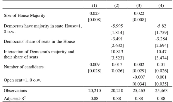
Secondly, we use an instrumental variable procedure for the amount limit on contributions from individuals. In one two-stage least square regression we use the size of the state Assembly legislative majority, measured as the absolute difference in the number of seats between the Democrat and Republican party, as instruments. States differ in the size of their legislatures. For example, in 2000, Pennsylvania’s Assembly seated 203 legislators and Indiana’s Assembly seated 100 legislators. Thus the difference in the number of seats between the majority party and minority party may differ across two states even though their share of seats is the same in each legislature. The instrument is valid if it is correlated with contribution laws but uncorrelated with the error term in the second stage. With respect to the first requirement, our model suggests that if a party has a large majority in the state legislature, then this party is drawing from a larger pool of high quality candidates than the opposition party. Having many high quality candidates, the majority party has an incentive to vote for relaxed limits so that it can better advertise that it has high quality candidates. Thus we predict that the size of the majority is positively correlated with higher contribution limit amounts. With respect to the second requirement there is little reason to believe that the size of the majority in the legislature is correlated with the margin of victory in individual races. Even if one party were to obtain all the seats, this would not allow any deduction regarding the size of the margins of victory of the winning candidates. Furthermore, the difference in seats is not only determined by the fraction of races won by each party, but by the size of the legislature as well. Thus we use the size of the legislative majority as one of our instruments for contribution restrictions. We measure the majority size as the absolute difference between the seats held by Democrats and Republicans in the state Assembly.
Our second instrument is motivated by the recent discussion of federal campaign finance laws in which Democratic Assembly and Senate leaders favored stricter campaign finance limits while
Republican leaders opposed them. Our second instrumental variable approach includes three variables. One variable measures whether Democrats had a majority in the state Assembly, a second variable measures the share of Democratic seats in the state Assembly, and a third variable is an interaction between the first two. The reason we use these three variables is that Democrats may favor limits when they are the minority, but may oppose limits when they are the majority. Thus, including the share of the Democratic seats in the Assembly and an interaction term will allow for such a strategy. Furthermore, including these variables will allow us to test for overidentifying restrictions.
Several other variables may affect the competitiveness of state races as well. For example, states differ with respect to political traditions and outcomes. Thus, roughly similar regulatory regimes may produce dissimilar results due to differences in the political culture in those states. This analysis takes into account the differences in political traditions across states via state indicator variables.
district competitiveness that is associated with redistricting. Second, the state indicators allow for the possibility that some states are more rigorous in their redistricting decisions, resulting in more
competitive races. In a subset of our estimates we are employing district fixed effects. Since we were unable to identify which assembly districts changed their shape in 1992, our district fixed effects are based on district boundaries in the 1980s.
The interpretation of the CFLAW variable is problematic if, in response to stricter limits on contributions, political parties recruit more challengers. In that case, the election is more competitive after passage of the limit, but the competitiveness is caused not by less spending but rather by altered party behavior. Therefore we control for the number of challengers in some of our regression
specifications.
In the 1990s, campaign finance innovations emerged including independent expenditures, party soft money, and leadership funds. Though these activities are prominent at the federal level, they are less important in state Assembly legislative races. To the extent that these activities exist as substitutes for a tightening of campaign finance regulation, they would make it more difficult for us to find an effect of campaign finance laws on election outcomes. We will capture the national trend in these activities via year indicators.
Some groups, for example PACs, may circumvent limits by supporting their candidates in alternative ways, such as issue advertisements. Although this may be an issue at the federal level, PACs run issue ads in few state Assembly districts. PACs undertaking activities to offset existing regulations imply that the estimated effect will be attenuated. The fact that PACs may undertake such activities constitutes an omitted variable problem, but we can obtain consistent coefficients with our two-stage least square methods.
IV. Data Issues
We obtained data on general elections in state Assembly single member districts from the Inter-University Consortium for Political and Social Research (ICPSR) for 1980-1989 and 1993-1994.9 We obtained the state data for the 1990-1992 and 1995-2001 years from each state’s Elections Division or its State Board of Elections. We focus on single member districts since over 80 percent of all state legislators are elected to these districts. Since at the federal level all Assembly districts are single member districts, the focus on single member districts also makes it easier to transfer knowledge from the state to the federal level.10
Our source for the campaign finance laws is the biannual publication, Campaign Finance Law.11 In Table A1 of the appendix we report which states limited individual, PAC, union, corporate,
9
We had to make some corrections to the ICPSR data set since some of its organization was not suitable for this work. For example, in some states, some candidates appeared twice as running for the same district and we combined those records. We spot-checked and found no mistakes in the remaining data.
10
In some states and districts competition for the legislative seats occurs primarily at the party level and, thus, in the primary election rather than in the general election. In this case it is advantageous to study primaries. ICPSR provides primary data only for southern states and for a limited time period. Though a data collection effort to supplement ICPSR data is clearly important, it is beyond the scope of this study.
11
or party contributions for state Assembly candidates and which states did not. If a state switched from one regime to another, we report the first election year for when the new contribution law applied.12 Table A1 shows that a relatively large number of states changed their campaign finance laws in the 1980s and 1990s. For example, the number of states regulating individual contributions has been steadily rising from twenty-two states in 1980 to thirty-four states in 2001. There also has been a similar pattern for PAC, corporate, union and party contributions.
Individual contributions account for the vast majority of total contributions. When candidates’ sources of funds are categorized into “parties,” “PACs,” “public funding,” “self,” and “others including individuals,” in Idaho over 90 percent of the funding sources are from the “others including individuals” category (Malbin and Gais, 1998 p.154ff). This category includes individual contributions by, for instance, CEOs of corporations and labor leaders, but not direct contributions from corporations or labor organizations. The state with one of the lowest percentages in this category is Minnesota, but even there this category amounts to approximately 45 percent of all funding sources (Malbin and Gais, 1998 p.154ff). Party contributions constitute only a small percentage of candidate funding (Gierzynski and Breaux 1991), while the contribution pattern in states examined by Malbin and Gais (1998) showed that in no state did corporate, labor and political action committee contributions together amount to more than thirty percent of all contributions (Malbin and Gais, 1998 p.154ff). Therefore, in some of our regressions, we focus on individual contribution regulations since these contributions are quantitatively the most important in state elections. In other regressions we employ the aforementioned index of whether a state has limits on contributions from individuals, PACs, corporations, unions, or parties.
Table 1 shows the proportion of states that have enacted contribution restrictions on campaign contribution for individuals, PACs, corporations, unions, and parties and shows that these restrictions are highly positively correlated, suggesting that when states limit individual contributions, they tend to put limits on PAC and other contributions at the same time.13 For example, the correlation coefficient between limited individual and PAC giving is 0.81, and between laws that limit union and corporate contributions it is 0.75. The high correlation coefficients suggest that when states implement limits, they implement limits for most categories of giving. Thus, if we were to include all laws in one regression equation, the regression may not be able to precisely identify the marginal effect of each category, and the estimation results may be imprecise due to co-linearity. Therefore, we will analyze the effect of restrictions with an index.14 When examining the effects of contribution limit amounts, we will focus on this Campaign Finance Law publication The precursor was of this publication was Campaign Finance Law 1981. We obtained data for 1980 from this source. For 1982, we consulted the all state statues, and determined whether laws changed from unlimited contributions to limited contributions between 1980 and 1982. All law changes are illustrated in the Table A1.
12
We compared the classifications in Campaign Finance Law to the classification in Malbin and Gais (1998) who shared their law data with us, and found a large overlap. In two cases (Georgia and Ohio) the sources provided different information as to whether a limit was implemented and in those cases we consulted the state statutes.
13
A similar picture emerges when one examines the contribution limit amounts.
14
limits on individual giving, given that these limits are by far the quantitatively most important source of contributions in state Assembly races.
Our data set includes forty-five of the fifty states. Since the empirical analysis focuses on single member districts, Arizona, New Jersey, and North Dakota are omitted from this data set because all of their state legislators run in multi-member districts. Nebraska is omitted because its elections are staggered. Louisiana is omitted since its relevant competition occurs in primaries, and sometimes there is no general election depending on the outcome of the primary.15
Assuming that contribution limits affect the amount of campaign expenditures, contribution limits have a direct effect on vote shares. There is some evidence that stricter contribution limits lead to lower expenditures. Hogan (2000), for example, documents that state campaign contribution restrictions reduced spending in the 1994 state legislative races. Additionally, we correlated campaign spending per candidate, collected by the National Institute on Money in State Politics, with 1998 state
contribution restrictions and found less spending in states with stricter contribution limits, lending further support to the claim that limits are binding and that relaxed limits lead to greater spending.
V. Results
Table 2 presents the means and standard deviations of the variables employed in the two samples of the analysis. One sample contains only races where one of the candidates is an incumbent (Table 2, column 1). The other sample includes all races (Table 2, column 2). The table shows that between 1980 and 2001, fifty-six percent of the district races are subject to individual contribution limits.
We created a “pre-limit incumbent” variable. For individual contribution limits this “pre-limit incumbent” variable equals zero in the years of unrestricted contributions from individuals, and equals one after implementation of the contribution limit law for those legislators who were a member of the state Assembly before the contributio n restrictions were passed. For example, for individual contribution limits, this variable equals one in six percent of the district races (Table 2, column 1). We will include this variable in some regression specifications to address one of the endogeneity concerns and to test whether restrictions’ effects differ across incumbent cohorts.
The variable “contribution limit amount” is measured in thousands of 1998 dollars and has fewer observations than the contribution limit indicator variable because some states do not have a
contribution limit. In states with limits, the average contribution limit per district race is $3,200. The average incumbent vote share is seventy-eight percent, indicating that incumbents tend to win by overwhelming margins. The margin of victory variable measures the difference in the vote share
obtained by the winning candidate and the runner up. On average there are 1.8 candidates per race for a seat in the state Assembly. In our data set incumbents are uncontested in approximately thirty-five percent of all races.
15
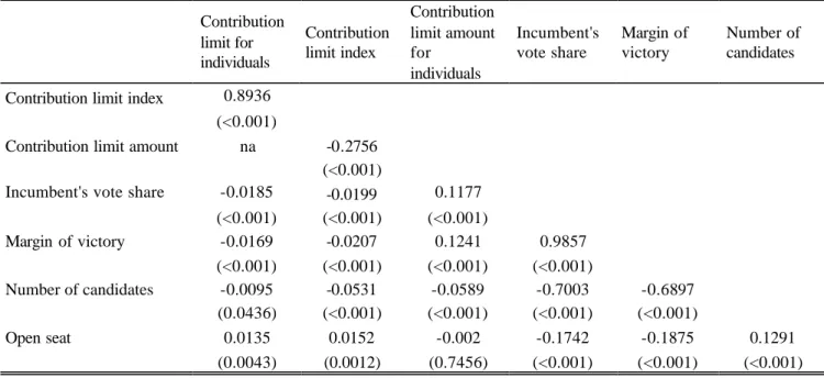
Table 3 shows the correlation matrix for the main variables used in the regression equations. The raw correlations indicate that elections are closer in states with contribution restrictions on individuals and that incumbents receive lower vote shares when these limits are in place.16 Higher individual contribution limit amounts are associated with less close elections, larger incumbent vote shares, and fewer candidates running for office. Clearly, these correlations are only suggestive. We next estimate a statistical model that examines whether a causal connection can be established between campaign finance laws and election outcomes.
Table 4 shows the estimation result corresponding to equations (1) and (2). In these
regressions, the dependent variable is the margin of victory in races with incumbents. In our sample over ninety-five percent of the incumbents win reelection, thus the dependent variable is essentially the incumbent’s margin of victory.17 The first regression includes the individual contribution law indicator and state and year fixed effects (Table 4, column 1). We add the pre-limit incumbency variable to the second regression (Table 4, column 2). In these regressions the CFLAW coefficient measures the effect of the contribution limit for those legislators who were not present when the law was passed. One potential concern with the first two specifications is that contribution restrictions may draw more candidates into races and that the estimates on the CFLAW coefficients are due to a larger number of candidates when the restrictions are in place. Thus, in the third specification we control for the number of candidates (Table 4, column 3). As mentioned earlier, we also constructed a campaign contribution limit index that combines all five contribution laws. The estimation results that use the three
specifications just described but substitute the index for the law on individual giving are in Table 4, columns 9, 10, and 11.
In Table 4 the coefficients for contribution restrictions have the anticipated negative signs. For example, changing the law from having no limits on contributions from individuals to having limits leads to a reduction in the incumbent vote share between 3.3 and 6.0 percentage points.
In all specifications the pre-limit incumbent coefficient takes the opposite sign of the contribution law variables, indicating that the incumbents who passed the limited contribution law are less affected by the law than those who became incumbents after its passage.18 For example, the coefficients in column 2 imply that the margin of victory of pre-limit incumbents narrows by 3.5 percentage points after passage of the individual contribution limit, while the margin of victory of future incumbent generations narrows by over six percentage points. This difference is statistically different from zero. Thus, we conclude that contribution limits reduce the vote shares of all incumbents, but they reduce the vote shares of future incumbent generations more than they reduce the vote shares of those incumbents who passed the law.19
16
The correlation coefficient between the closeness of the election and on whether there are limited PAC contributions, union contributions, and party contributions is also negative and statistically significant, whereas the correlation coefficient is positive for corporate contributions limits.
17
When we estimate these models with only incumbents who won the election, the estimation results are very similar to those reported in Table 4.
18
This finding is also consistent with the hypothesis that low quality incumbents get defeated, so the remaining incumbents have a higher margin of victory.
19
Controlling for the number of candidates reduces the magnitudes of the contribution limit coefficients, but the coefficients remain negative and statistically significant (Table 4, column 3). Furthermore, we continue to find a differential effect of the limits for new incumbents and incumbents who passed the law. The contribution limit coefficients are smaller in the third specification than in the second specification because the number of candidates variable is correlated with contribution limits (Table 3). The size of the number of candidates’ coefficient indicates that one more candidate reduces the margin of victoryby about thirty-nine percentage points, which appears large, but is primarily driven by the fact that a previously uncontested incumbent has a challenger from a main opposition party who draws a large number of votes.2021
We also estimated the same set of regressions in Table 4 with the incumbents’ vote share as the dependent variable (not reported in the Tables). The significance levels are similar to those reported in Table 4, and as one would expect when a race involves only two candidates, the size of the coefficients on the contribution laws in the incumbents’ vote share regressions is half of what it is in the margin of victory regressions. This is due to the fact that almost all races are two candidate races, and when the margin of victory is reduced by ten percentage points, the incumbents vote share typically falls by five percentage points.
When employing the contribution law index variable in our regressions (Table 4, columns 9, 10, 11), using the same specifications as for the individual contribution law variable, we find similar results as those discussed previously. We also estimated the regressions by employing district fixed effects (Table 4, column 4, 5, 12, 13). The magnitudes of the coefficients on contribution limits are slightly reduced when we include district fixed effects and the point estimates remain statistically significant. Not surprisingly these effects account for over eighteen percent of the variation in the data, as indicated by the increase in the R-squared from columns 2 to 4. To test whether our results are robust with respect to the inclusion of the lagged margin of victory of the incumbent, we included this variable in Table 4, columns 6, 7, 14 and 15. In these regressions all point estimates on contribution limits have the
anticipated negative sign and are statistically significant at the ten percent level in three out of four cases. Finally, we eliminated the uncontested races and estimated the regression for the contested races only in Table 4 column 8, which shows that the estimates are robust in this restricted sample.
Table 5 substitutes the individual dollar contribution limit variable for the campaign contribution limit indicators, controlling for number of candidates and previous margin of victory. In columns 1 and 2 we find that a higher dollar contribution limit leads to an increase in the margin of victory of the race, although the OLS point estimates are not statistically significant. In columns 3 and 4 we include an reelection, while low quality incumbents do not.
20
When we use a logistic transformation of our dependent variable, our qualitative and quantitative results are similar to those reported in the table.
21
We examined whether our results are sensitive to the inclusion of time-varying state
indicator for whether a state has limits and its interaction with the dollar limit amount.22 Columns 3 and 4 show that election margins are significantly lower in states with limits and that the looser the dollar limit, the wider the margin.
One potential concern with these estimates is that the contribution limit is endogenous because omitted variables may simultaneously affect vote shares and the contribution limit amount. Columns 5 to 10 of Table 5 address this concern by estimating 2SLS regressions. Columns 5 and 6 use the size of the Assembly majority, measured as the absolute difference in the number of seats between the Democrat and Republican party as the instrument, whereas columns 7 to 10 use Democrat control variables, both with state and district fixed effects.23 The corresponding first stages are shown in Table A2 of the appendix. The first stage regressions that use Democrat control variables show that
Democrats favor tighter limits, but only if they are the minority or have a slim majority. The regression results imply that Democrats favor more generous limits when they have a majority exceeding about fifty-five percent.24
The regressions in Table 5 show that our previous results are robust when we use 2SLS methods. Five out of six estimated coefficients on the contribution amounts are statistically significant at the five percent level. In most specifications, the contribution limit coefficients more than double in size when compared to the OLS estimates. That the OLS coefficient is biased downwards is consistent wit the previously discussed hypothesis that voters press for tighter limits when elections become less competitive, which may be the result of an increased incumbency advantage. When controlling for the number of candidates in the race, reducing the limit from $3,000 to $2,000 lowers the margin of victory by four percentage points (Table 5 column 5). Given that regressions 7 to 10 in Table 5 use several instruments, we can test for overidentifying restrictions. Those tests support the hypothesis that the Democrat control variables are valid instruments. The last two columns of Table 5 estimate 2SLS regressions with district fixed effects and lagged margin of victory. 25
Whether the estimated effects of contribution limits are large has to be evaluated with the understanding that the average contribution limit in this sample is about $3,200 and that the average incumbent receives over seventy five percent of the popular vote. Thus, even significantly reducing an existing $3,000 limit will not put the average incumbent into a close race. Although stricter limits
22 The specification used is β
1CFLAW + β2CFLAW*(dollar limit), where CFLAW is an indicator that
equals one when there are contribution limits, as in Table 4. The dollar limit is coded so that in states without limits, the interaction term equals zero.
23
We also examined two other instruments, such as the size of the Assembly majority measured as the percentage difference in the number of seats, and the presidential two-party vote for each state. In both cases our results were similar to those reported in this paper.
24
We do not report the first stages of some of the subsequent 2SLS regressions sinc e they are very similar to those reported in the Appendix.
25
increase the competitiveness of elections, their overall effect on incumbent turnover rates is rather limited.26
As noted previously, in our sample, 95 percent of the incumbents win the elections. By
examining the vote shares obtained by winning incumbents, we calculated how many incumbents would have lost if the contribution limit were reduced by $2,000. Our point estimate implies that this would lead to a narrowing of the margin of victory by approximately seven percent (Table 5, column 7). When applying this estimate we find that approximately five percent of all winning incumbents would have lost the general election if contribution limits were curtailed by $2,000.
Table 6 addresses the impact of contribution limits on incumbent’s victory or defeat. The dependent variable in these regressions equals one if the incumbent won the election and zero otherwise. We estimate conditional logit models with district and year effects, controlling for number of candidates. Individual contribution limits reduce the incumbent’s probability of winning, but the coefficient is
statistically insignificant (column 1). However, the contribution limit index reduces that probability with a ten percent significance level (column 2). Columns 3 and 4 include dollar contribution limits. The sum of these results indicates that even if contribution limits reduce incumbent’s margins, they only barely produce incumbent defeats. The biggest threat to incumbents is increased entry into the electoral race, as indicated by the negative and statistically significant coefficient on the number of candidates.
In Table 7 we examine both races with incumbents and open seat races and the dependent variable is the margin of victory of the winner—and not the margin of the district election, as in Tables 4 and 5. We continue to find that the introduction of contribution limits for individuals reduces the margin of victory and affects the incumbent generation responsible for passing the law less than it affects subsequent incumbent generations (Table 7, columns 1 to 4). We find similar results for the contribution limit index (columns 5 and 6).
Facing contribution limits, incumbents may decide not to run for reelection because limits reduce their competitive advantage. Such decisions, of course, generate open seats. Thus, to some extent open seats are induced by tighter limits, which explains why the size of the limit coefficient gets smaller when the open seat variable is included (Table 7 columns 2, 4 and 6). Similarly, the finding that the
contribution limit coefficient is getting smaller when the number of candidates is included may be due to the high correlation between these variables (see Table 3). To the extent that limits cause more
candidates to enter the race, the magnitude of the contribution limit coefficient is understated when the number of candidates is included in the regression equation. Table 7 shows that open seats elections are more competitive, even when controlling for the number of candidates.27
26
Because the relationship between dollar contribution limits and vote shares may be nonlinear, we added the squared contribution amount to models 3 and 4 of Table 5. The results showed some evidence that, conditional on having limits, looser limits increase margins of victory at a decreasing rate, which reaches a maximum at about ten thousand dollars. In our sample, six states had limits higher than $10,000.
27
We also examined the impact of restrictions in open races only. If limits restrict the brand name development of incumbents, one would expect limits to reduce the margin of victory in races with
The last four columns in Table 7 substitute the individual contribution limit amount for the contribution limit indicator variable. More restrictions on giving lead to closer elections, both in the OLS and 2SLS specifications. We find that a tightening of contribution limits by $1,000 makes election closer by three percent (Table 7, column 8 and 9). As before, we can not reject the null hypothesis for overidentifying restrictions, which supports the validity of our instruments.
Our data do not allow for discriminating between the hypothesis that limits lead to closer elections, because they reduce the amount of information that high quality candidates can get to voters, and the hypothesis that limits lead to closer elections because they curtail the incumbency advantage. However, while the candidate quality model does not offer predictions regarding the number of candidates entering the race, the hypothesis that limits reduce the incumbency advantage implies that incumbents will face more challengers when contribution limits are in place. This issue is addressed in Table 8.
Table 8 examines whether the number of candidates is positively or negatively related to
campaign contribution restrictions. Excluding the open seat variable, we find that individual limits lead to a 0.11 increase in the number of candidates in district elections. However, we find that there is no increase in competition for legislators who passed the contribution limit law (Table 8, column 1 and 3). Using the contribution limit index variable we find similar results regardless of whether we exclude the open seat variable. The OLS results for contribution limit amounts do not support the previous findings that stricter limits draw extra candidates into elections. The corresponding 2SLS point estimates are significant and similar regardless of whether we use the Assembly majority or democratic control instruments. The largest 2SLS estimate suggests an increase by 0.1 candidates for a $1,000 reduction in an individual contribution limit.
VI. How do limits alter the competitiveness of elections?
The findings in this paper establish that contribution limits lead to closer elections, and the results are consistent with both the hypothesis that limits hurt high-quality incumbents and the brand name hypothesis. However, the results do not shed light on the underlying mechanism. Limits may be associated with more competitive challengers because limits curtail incumbents’ fundraising ability or high quality incumbent’ ability to raise funds. However, it is possible that contribution limits do not affect campaign contribution patterns at all, and that limits may be linked to other mechanisms causing closer elections.
The hypothesis that contribution limits hurt high quality candidates implies that contribution limits lead to fewer contributions to incumbents (assuming incumbents are high quality, on average) and to a smaller contribution gap between incumbents and challengers (assuming challengers are low quality, on average). Thus, the hypothesis implies that the gap is caused by lower contributions to incumbents, not by higher contributions to challengers. The hypothesis that contribution limits reduces the incumbents’ fundraising advantage also implies that incumbents receive fewer contributions.
To test for these implications, we collected camp aign contribution data for main party
incumbents and main party challengers for the 1998 state Assembly elections.28 First, we test whether
28
the share of incumbent contributions as a share of total contributions is lower in states with stricter contribution limits. We find that the share of incumbent contributions is lower in states with stricter contribution limits.29 The point estimate on the contribution limit index coefficient has a negative sign and is statistically significant at the seven percent level, indicating that when states switch from no limits to having limits on all five types of contribution sources, incumbents’ share of total contributions in an electoral race is lowered by six percent (the mean incumbent contribution share is seventy-seven percent). To determine whether this finding is generated by increased challenger contributions or by lower incumbent contributions we estimate two regressions with either incumbent or challengers contributions as the dependent variable. We find that challenger contributions do not differ between states with an without limits, but that contributions to incumbent are lower in states with limits and that the associated point estimate is statistically significant at the six percent level.30 Finally, we examine the dollar gap in contributions between incumbent and challengers and find that the contribution gap narrows with stricter limits.
Clearly, the results have to be interpreted with caution, as they do not stem from a panel analysis but from a cross-section. However, they do suggest that contribution limits lead to changes contribution patters and these changes in patters are consistent with the mechanism described in models predicting that limits lead to more competitive elections.
VI. Conclusion
We examined whether and how campaign finance laws affect incumbent vote shares, closeness of elections, and the number of candidates in an election. We focused on state single member districts between 1980 and 2001 and found support for models that predict that contribution limits narrow the margin of victory of incumbents. Our results show that the introduction of contribution limits decreases the margin of victory, which in turn increases the closeness of elections. Tightening already existing contribution limits makes races closer and reduces the incumbency advantage. Our estimates imply that the introduction of contribution limits increases the closeness of an election for races with incumbents by up to six percentage points (Table 4, column 2 and 4). In our incumbent sample of about 36,000 district elections, a few more than 1,400 incumbents won with a margin of victory of less than six percent. These numbers indicate that the enactment or tightening of campaign finance laws does not lead to a large increase in incumbent turnover. These estimates also suggest that the recent increase in federal individual contribution limits, brought by the Bipartisan Campaign Reform Act of 2002 is most likely to benefit incumbents at the expense of challengers.
However, these effects of contribution restrictions are smaller for the legislators who passed contribution limits. When incumbent legislators decide to let inflation erode limits or to pass legislation curtailing contribution limits, they do so without significantly reducing their expected vote shares. However, contribution limits do reduce the vote shares of future incumbent generations. Contribution available only for recent years. We collected data for thirty-eight states.
29
In these regressions we allow for clustering of observations by state and include state population and state income as control variables. The number of observations in these regressions is 1,618.
30
limits increase the number of candidates in elections, but again this effect holds primarily for future incumbent generations; legislators who pass this legislation are not subject to increased competition.
These results indicate that contribution limits are not incumbency protection devices but that limits lower incumbents’ margins at the polls. These findings support the models that predict that limits make elections more competitive. We have also shown that limits increase the number of candidates in electoral races. This finding lends support to the hypothesis that limits reduce the incumbency
advantage. Our results from a cross-section of campaign contributions to candidates suggest that limits indeed weaken the incumbent’s fundraising ability and that they help the challenger because the
References
Angrist, Joshua D. “Grouped-data estimation and testing in simple labor-supply models,” Journal of Econometrics, 1991, 47, 243-66.
Ansolabehere, Stephen, John M. de Figueredo, and James Snyder. “Why is There so Little Money in U.S. Politics?” Journal of Economic Perspectives, 17(1), Winter 2003, 105-130.
Austen-Smith, David, “Interest Groups, Campaign Contributions and Probabilistic Voting, ” Public Choice, 1987, 54, 123-39.
Bronars, Stephen G. and Lott, John R. Jr., “Do Campaign Donations Alter How a Politician Votes? Or, Do Donors Support Candidates Who Value the Same Things That They Do?” Journal of Law and Economics, 40, 2, October 1997, 317-350.
Coate, Stephen, “Political Competition with Campaign Contributions and Informative Advertising,” 2001, NBER Working Paper #8693.
Coate, Stephen, “Power-hungry Candidates, Policy Favors, and Pareto Improving Campaign Contribution Limits,” mimeo, Cornell University, 2002.
Feigenbaum, Edward D. and James A. Palmer, Campaign Finance Law, Federal Election Commission, bi-annual issues, 1980-2000.
Gierzynski, Anthony, and David Breaux, “Money and Votes in State Legislative Election,” Legislative Studies Quarterly, 1991, 16, 203-17.
Green, D. and Krasno, J. “Salvation of the Spendthrift Incumbent: Reestimating the effects of campaign spending in House elections,” American Journal of Political Science, 32, 1988, 363-72.
Grier, Kevin B. “Campaign Spending and Senate Elections, 1978-84” Public Choice, 63(3), 1989, 201-220.
Grier, Kevin B. and Michael C. Munger, "Committee Assignments, Constituent Preferences, and Campaign Contributions," Economic Inquiry, January 1991, 29, 24-43.
Gross, Donald A., Robert K. Goidel, and Todd G. Shields, “State campaign finance regulations and electoral competition, March 2002, American Politics Research, 30, 2, 143-65.
Hogan, Robert, “The Costs of Representation in State Legislatures: Explaining Variations in Campaign Spending,” Social Science Quarterly, December 2000.
Kettl, Donald, et al. “Report of the Commission, vol. I” Governor’s Blue-Ribbon Commission on Campaign Finance Reform, State of Wisconsin, 1997.
Kousser, Thad and Ray LaRaja, “How Do Campaign Finance Laws Shape Fundraising Patterns and Electoral Outcomes? Evidence from the States,” Working paper, 2000.
Kroszner, Randall S. and Thomas Stratmann. “Interest Group Competition and the Organization of Congress: Theory and Evidence from Financial Services’ Political Action Committees,” American Economic Review, 88, December 1998, 1163-87.
Levitt, Steven. “Using Repeat Challengers to Estimate the Effect of Campaign Spending on Election Outcomes in the U.S. House.” Journal of Political Economy 103, August 1994, 777-98.
Lott, John R. “The Effect of Nontransferable Property Rights on the Efficiency of Political Markets,” Journal of Public Economics, 31(2), 1987, 231-46.
Malbin, Michael J. and Gais, Thomas L., The Day After Reform: sobering campaign finance lessons from the American states. Rockefeller Institute Press, 1998.
Mayer, Kenneth. Public Financing and Electoral Competition in Minnesota and Wisconsin, University of Southern California, 1998.
Milyo, Jeffrey “The Economics of Campaign Finance: FECA and the Puzzle of the Not Very Greedy Grandfathers”, Public Choice, 1997, 93, 245-270.
Milyo, Jeffrey, David Primo, and Timothy Groseclose. “The effects of State Campaign Finance Regulation on Turnout, Electoral Competition, and Partisan Advantage in Gubernatorial Elections, 1949-1998,” mimeo, 2002.
Milyo, Jeffery and Timothy Groseclose, "The Electoral Effects of Incumbent Wealth," Journal of Law and Economics, 42(2), October 1999, 699-722.
Mueller, Dennis C. and Thomas Stratmann "Informative and Persuasive Campaigning," Public Choice, 81(1), October 1994, 55-77.
Ortuno-Ortin, Ignacio and Christian Schultz, “Public Funding for Political Parties,” CESifo Working Paper No. 368, 2000.
Potters, Jan, Randolph Sloof and Frans van Winden, “Campaign Expenditures, Contributions, and Direct Endorsements: The Strategic Use of Information and Money to Influence Voter Behavior,” European Journal of Political Economy, 1997, 13, 1-31.
Prat, Andrea,, “Campaign Spending with Office-Seeking Politicians, Rational Voters, and Multiple Lobbies,” Journal of Economic Theory, 2002b, 103(1), 162-189.
Ramsden, Graham P. “State Legislative Campaign Finance Research: A Review Essay,” State Politics and Policy Quarterly, 2(2), Summer 2002, 176-198.
Redfield, Kent D., Ca$h clout: political money in Illinois legislative elections. University of Illinois at Springfield, 1995.
Redfield, Kent D. Money counts: how dollars dominate Illinois politics and what we can do about it. Institute for Public Affairs, University of Illinois at Springfield, 2001.
Snyder, James M., Jr. “Long-term Investing in Politicians: or, Give Early, Give Often.” Journal of Law and Economics 35, April 1992, 15-43.
Smith, Bradley A. "Campaign Finance Regulation: Faulty Assumptions and Undemocratic Consequences" Cato Policy Analysis no. 238, September 13, 1995.
Stratmann, Thomas, “What Do Campaign Contributions Buy? Deciphering Causal Effects of Money and Votes.” Southern Economic Journal, 57, 1991, 606-64.
Stratmann, Thomas. “Are Contributions Rational? Untangling Strategies of Political Action Committees.” Journal of Political Economy 100, 3, 1992, 647-64.
Stratmann, Thomas, "Campaign Contributions and Congressional Voting: Does the Timing of Contributions Matter?" Review of Economics and Statistics, February 1995, 72 (1).
Stratmann, Thomas, "The Market for Congressional Votes: Is the Timing of Contributions Everything?" Journal of Law and Economics, April 1998, 41, 85-114.
Thompson, Joel A. and Moncrief, Gary F., eds. Campaign Finance in State Legislative Elections. Congressional Quarterly Books, 1998.
TABLE 1
Correlation Matrix of State Contribution limits
Individual contribution limit PAC contribution limit Corporation contribution limit Union contribution limit Mean (Std. Dev.) Individual contribution limit 0.5921 (0.4920) PAC contribution limit 0.8096 (<0.001) 0.4979 (0.5005) Corporation contribution limit 0.7290 (0.1783) 0.5996 (<0.001) 0.7218 (0.4486) Union contribution limit 0.7880 (<0.001) 0.7792 (<0.001) 0.7448 (<0.001) 0.5900 (0.4924) Party contribution limit 0.4909 (<0.001) 0.6170 (<0.001) 0.3606 (<0.001) 0.4932 (<0.001) 0.2741 (0.4465)
TABLE 2
Means and Standard Deviations
Incumbent
Sample All Races
0.562 0.564
Individual contribution limit = 1, 0 otherwise
(0.496) (0.496)
0.060 0.048
Pre-limit Incumbent in years after limit became
law = 1, 0 otherwise (0.237) (0.213)
2.660 2.674 Contribution limit index a
(2.009) (2.017) 0.388 0.310 Pre-limit Incumbent in years after limits became
law (index) (1.124) (1.016)
3.227 3.223
Individual contribution limit amount, in 1998
thousands of dollars b (3.153) (3.184)
78.202 -
Incumbent’s vote share
(19.78) -
57.80 54.22
Margin of victory for the winning candidate
(37.65) (38.04)
60.75 -
Previous margin of victory for incumbent
candidate c (36.640) -
- 0.202
Open seat = 1, 0 otherwise
- (0.401)
1.761 1.806
Number of candidates per district
(0.684) (0.690)
Number of observations 35,998 45,084
Notes:
a. Index is the sum of dummy variables for whether individuals, corporations, unions, PACs, and political parties face contribution limits.
TABLE 3 Correlation Matrix
Contribution limit for individuals
Contribution limit index
Contribution limit amount for
individuals
Incumbent's vote share
Margin of victory
Number of candidates
Contribution limit index 0.8936 (<0.001)
Contribution limit amount na -0.2756 (<0.001)
Incumbent's vote share -0.0185 -0.0199 0.1177 (<0.001) (<0.001) (<0.001)
Margin of victory -0.0169 -0.0207 0.1241 0.9857
(<0.001) (<0.001) (<0.001) (<0.001)
Number of candidates -0.0095 -0.0531 -0.0589 -0.7003 -0.6897 (0.0436) (<0.001) (<0.001) (<0.001) (<0.001)
Open seat 0.0135 0.0152 -0.002 -0.1742 -0.1875 0.1291
(0.0043) (0.0012) (0.7456) (<0.001) (<0.001) (<0.001)
TABLE 4
Effects of Campaign Finance Restrictions on Vote Margins: Races with Incumbents Standard errors below coefficient estimates
(1) (2) (3) (4) (5) (6) (7) (8)
-4.413 -6.024 -3.29 -5.737 -3.603 -3.606 -1.508 -9.258 Contribution limit for individuals = 1, 0
otherwise [1.494] [1.793] [1.744] [1.954] [1.766] [1.732] [1.639] [2.468]
2.509 1.759 2.443 1.706 -0.036 0.328 3.625 Pre-limit incumbent in years after limit
became law = 1, 0 o.w. [1.359] [1.123] [1.752] [1.339] [1.362] [1.211] [1.654]
-39.26 -37.001 -37.567
Number of candidates
[2.108] [2.189] [2.079]
0.373 0.227 Previous margin of victory
[0.008] [0.012]
Includes year effects Yes Yes Yes Yes Yes Yes Yes Yes
Includes state/district effects State State State District* District* State State State
Period / sample 1980-2001 1980-2001 1980-2001 1980-2001 1980-2001 1982-2001 1982-2001 Contested races only
Observations 35,998 35,998 35,998 35,998 35,998 24,116 24,116 23,087
Adjusted-R2 0.15 0.15 0.55 0.33 0.64 0.27 0.61 0.16
TABLE 4 continued
(9) (10) (11) (12) (13) (14) (15)
-0.885 -1.557 -1.094 -1.393 -0.961 -0.709 -0.739 Contribution limit index
[0.342] [0.389] [0.387] [0.416] [0.395] [0.378] [0.357]
1.06 0.677 0.808 0.545 0.083 0.29
Pre-limit incumbent in years after limit
became law = 1, 0 o.w. [0.297] [0.251] [0.351] [0.301] [0.310] [0.272]
-39.257 -37.001 -37.575
Number of candidates
[2.108] [2.189] [2.078]
0.373 0.226 Previous margin of victory
[0.008] [0.012]
Includes year effects Yes Yes Yes Yes Yes Yes Yes
Includes state/district effects State State State District* District* State State
Period / sample 1980-2001 1980-2001 1980-2001 1980-2001 1980-2001 1982-2001 1982-2001
Observations 35,998 35,998 35,998 35,998 35,998 24,116 24,116
Adjusted-R2 0.15 0.15 0.55 0.33 0.64 0.27 0.61
TABLE 5
Effects of Individual Contribution Limit Amounts on the Margin of Victory: Races with Incumbents
Standard errors below coefficient estimates
(1) (2) (3) (4) (5) (6) (7) (8) (9) (10)
OLS OLS OLS OLS 2SLS 2SLS 2SLS 2SLS 2SLS 2SLS
0.425 0.376 0.662 0.562 4.037 1.985 3.403 1.567 4.487 3.36 Contribution limit amount for
individuals [0.263] [0.295] [0.240] [0.256] [1.842] [0.853] [1.455] [0.880] [0.542] [0.583]
0.24 0.226 0.239 0.239 0.061
Previous margin of victory
[0.019] [0.012] [0.019] [0.019] [0.007]
-4.599 -3.324 Individual limit exists=1
[1.792] [1.721]
-39.426 -36.497 -39.266 -37.58 -39.387 -36.488 -39.394 -36.49 -36.752 -36.696 Number of candidates
[3.494] [3.342] [2.107] [2.079] [3.493] [3.344] [3.494] [3.344] [0.322] [0.387]
Includes year effects Yes Yes Yes Yes Yes Yes Yes Yes Yes Yes
Includes state/district effects State State State State State State State State District* District*
Instruments - - - -
Size of House Majority
Size of House Majority
Democrat control variables
Democrat control variables
Democrat control variables
Democrat control variables
Observations 20,213 13,665 35,998 24,116 20,213 13,665 20,213 13,665 20,213 13,665
Adjusted-R2 0.55 0.61 0.55 0.61 0.54 0.61 0.55 0.61 0.43 0.47
TABLE 6
Effects of Campaign Finance Restrictions on Incumbent Victory Standard errors below coefficient estimates
(1) (2) (3) (4)
-0.161 -0.226
Contribution limit for individuals = 1, 0 otherwise
[0.136] [0.170]
-0.054 Contribution limit index
[0.029]
0.041 0.019
Contribution limit amount for individuals
[0.033] [0.028]
-1.115 -1.114 -1.02 -1.114
Number of candidates
[0.075] [0.075] [0.123] [0.075]
Includes year effects Yes Yes Yes Yes
Includes district effects Yes Yes Yes Yes
Observations 10,713 10,713 5,732 10,713
Log likelihood -2,989 -2,988 -1,676 -2,988
Pseudo R2 0.096 0.096 0.082 0.096
TABLE 7
Effects of Campaign Finance Restrictions on the Margin of Victory: All Races Standard errors below coefficient estimates
(1) (2) (3) (4) (5) (6) (7) (8) (9) (10)
OLS OLS OLS OLS OLS OLS OLS 2SLS 2SLS 2SLS
-3.301 -1.426 -4.345 -2.229 Contribution limit for individuals = 1
[1.610] [1.626] [1.704] [1.702] 4.406 0.673 5.111 0.957 Pre-limit incumbent in years after limit
became law = 1 [0.959] [0.979] [1.195] [1.217]
-1.054 -0.557 Contribution limit index
[0.357] [0.353] 1.347 0.336 Pre-limit incumbent in years after limit
became law = 1 [0.230] [0.210]
0.393 3.157 2.629 3.192 Contribution limit amount for individuals
[0.253] [1.441] [1.167] [0.468] -10.137 -10.321 -10.051 -9.574 -9.548 -9.553 -9.746 Open seat = 1
[0.583] [0.580] [0.571] [0.911] [0.909] [0.908] [0.386] -38.415 -37.4 -36.499 -35.352 -38.378 -37.398 -38.284 -38.237 -38.246 -36.057 Number of candidates
[1.823] [1.820] [1.877] [1.868] [1.825] [1.821] [2.921] [2.921] [2.922] [0.279]
Includes year effects Yes Yes Yes Yes Yes Yes Yes Yes Yes Yes
Includes state/district effects State State District* District* State State State State State District*
Observations 43,208 43,208 43,208 43,208 43,208 43,208 24,344 24,344 24,344 24,344
Adjusted-R2 0.55 0.56 0.63 0.64 0.55 0.56 0.57 0.56 0.56 0.53
Notes: *District fixed effects subsume state effects. Standard errors are clustered by state-year in all regressions, except in column 10.
TABLE 8
Effects of Campaign Finance Restrictions on the Number of Candidates in All Races Standard errors below coefficient estimates
(1) (2) (3) (4) (5) (6) (7) (8) (9) (10)
OLS OLS OLS OLS OLS OLS OLS 2SLS 2SLS 2SLS
0.1152 0.0734 0.1118 Contribution limit for individuals =
1, 0 o.w. [0.0454] [0.0426] [0.0168]
-0.106 -0.0254 -0.1174 Pre-limit incumbent in years after
limit became law = 1, 0 o.w. [0.0284] [0.0262] [0.0195]
0.0224 0.0116 0.0252 Contribution limit index
[0.0097] [0.0093] [0.0036] -0.0321 -0.0103 -0.0327 Pre-limit incumbent in years after
limit became law = 1, 0 o.w. [0.0058] [0.0052] [0.0041]
-0.005 -0.09 -0.104 -0.0682 Contribution limit amount for
individuals [0.0076] [0.0482] [0.0470] [0.0348]
-0.004 Previous margin
[0.0002]
0.2178 0.2154 0.2155 0.2146 0.2145
Open seat = 1, 0 o.w.
[0.0094] [0.0095] [0.0129] [0.0133] [0.0134]
Includes year effects Yes Yes Yes Yes Yes Yes Yes Yes Yes Yes
Includes state/district effects State State District* State State District* State State State State Observations 45,084 45,084 45,084 45,084 45,084 45,084 25,466 25,466 25,466 13,665
Adjusted-R2 0.21 0.22 0.38 0.21 0.22 0.38 0.24 0.22 0.21 0.26
Notes: *District fixed effects subsume state effects. Standard errors are clustered by state -year in all regressions.
Appendix TABLE A1
State Contribution Laws for State House Races
Unlimited Contributions for entire time period
Switch from unlimited to limited contributions
Switch from limited to unlimited contributions
Limited contributions for entire time period
Individual contribution limit
AL, CA, IL, IN, IA, MS, NM, PA, TX, UT, VA
CO '98, GA '90, HI '82, ID '2000, MO '96, NV '92, OH '96, OR '96, RI '90, SC '92, TN '96, WA '94
CO 2000, MO 2000, OR '98
AK, AR, CT, DE, FL, KS, KY, MA, MD, ME, MI, MN, MT, NC, NH, NY, OK, SD, VT, WI, WV, WY
PAC contribution limit
AL, CA, IL, IN, IA, MS, NM, PA, SD, TX, UT, VA, WY
CO '98, GA '90, HI '82, ID '98, KS ‘82, KY '88, MA '94, MD '92, MO '96, NH '86, NV '92, NY '94, OH '96,OR '96, RI '90, SC '92, TN '96, WA '94
MO 2000, OR ‘98 AK, AR, CT, DE, FL, ME, MI, MN, MT, NC, OK, VT, WI, WV
Corporation contribution limit
CA, IL, IN, MO, NM, UT, VA CO '98, GA '90, HI ‘82, ID '98, NV '92, OR '96, RI '90, SC '92, WA '94
OR ‘98 AK, AL, AR, CT, DE, FL, IA, KS, KY, MA, MD, ME, MI, MN, MS, MT, NC, NH, NY, OH, OK, PA, SD, TN, TX, WI, VT, WV, WY
Union contribution limit
AL, CA, IL, IN, IA, MO, MS, NM, UT, VA
CO '98, GA '90, ID '98, KS '82, KY '92, MA '94, NV '92, NY '94, OH '96, OR '96, RI '90, SC '92, TN '96, WA '94, WI '84
OR ‘98 AK, AR, CT, DE, FL, HI, MD, ME, MI, MN, MT, NC, NH, OK, PA, SD, TX, VT, WV, WY
Party contribution limit
AL, CA, CT, DE, IL, IN, IA, KS, MD, MS, NC, NM, NY, PA, SD, TX, UT, VA, VT, WI, WY
AK '98, CO '98, FL '92, GA '90, HI '96, ID '98, KY '96, MA '96, MO '96, NH '96, NV '98, OH '96, OR '96, RI '94, SC '92, TN '96, WA '94
MO 2000, OR ’98, TN 98 AR, ME, MI, MN, MT, OK, WV
TABLE A2 First Stage Regressions Standard errors below coefficient estimates
(1) (2) (3) (4)
0.023 0.022
Size of House Majority
[0.008] [0.008]
-5.995 -5.82
Democrats have majority in state House=1,
0 o.w. [1.814] [1.759]
-3.491 -3.284
Democrats' share of seats in the House
[2.632] [2.694]
10.813 10.47
Interaction of Democrat's majority and
their share of seats [3.523] [3.474]
0.009 0.017 0.002 0.01 Number of candidates
[0.028] [0.026] [0.029] [0.026] -0.007 0.001 Open seat=1, 0 o.w.
[0.034] [0.035]
Observations 20,210 20,210 25,463 25,463
Adjusted-R2 0.88 0.88 0.88 0.88
Notes: Standard errors are clustered by state-year in all regressions.