Monetary Policy, Inflation,
and the Business Cycle
An Introduction to the New Keynesian Framework
Jordi Galí
Princeton University Press
Copyright © 2008 by Princeton University Press
Published by Princeton University Press, 41 William Street, Princeton, New Jersey 08540
In the United Kingdom: Princeton University Press, 6 Oxford Street, Woodstock, Oxfordshire OX20 1TW
All Rights Reserved
Library of Congress Cataloging-in-Publication Data Galí, Jordi, 1961–
Monetary policy, inflation, and the business cycle : an introduction to the New Keynesian framework / Jordi Galí.
p. cm.
Includes bibliographical references and index.
ISBN 978-0-691-13316-4 (hbk. : alk. paper) 1. Monetary policy.
2. Inflation (Finance). 3. Business cycles. 4. Keynesian economics. I. Title. HG230.3.G35 2008
339.5'3—dc22 2007044381
British Library Cataloging-in-Publication Data is available
This book has been composed in Times Roman by Westchester Book Group.
Printed on acid-free paper.∞ press.princeton.edu
Printed in the United States of America
Contents
Preface ix
1 Introduction 1
2 A Classical Monetary Model 15
3 The Basic New Keynesian Model 41
4 Monetary Policy Design in the Basic New Keynesian Model 71
5 Monetary Policy Tradeoffs: Discretion versus Commitment 95
6 A Model with Sticky Wages and Prices 119
7 Monetary Policy and the Open Economy 149
8 Main Lessons and Some Extensions 185
Preface
This book brings together some of the lecture notes that I have developed over the past few years, and which have been the basis for graduate courses on monetary economics taught at different institutions, including Universitat Pompeu Fabra (UPF), Massachusetts Institute of Technology (MIT), and the Swiss Doctoral Program at Gerzensee. The book’s main objective is to give an introduction to the New Keynesian framework and some of its applications. That framework has emerged as the workhorse for the analysis of monetary policy and its implications for inflation, economic fluctuations, and welfare. It constitutes the backbone of the new generation of medium-scale models under development at the International Monetary Fund, the Federal Reserve Board, the European Central Bank (ECB), and many other central banks. It has also provided the theoretical underpinnings to the inflation stability-oriented strategies adopted by the majority of central banks in the industrialized world.
A defining feature of this book is the use of a single reference model throughout the chapters. That benchmark framework, which I refer to as the “basic New Keynesian model,” is developed in chapter 3. It features monopolistic competition and staggered price setting in goods markets, coexisting with perfectly competitive labor markets. The “classical model” introduced in chapter 2, characterized by perfect competition in goods markets and flexible prices, can be viewed as a limiting case of the benchmark model when both the degree of price stickiness and firms’ market power vanish. The discussion of the empirical shortcomings of the classical monetary model provides the motivation for the development of the New Keynesian model, as discussed in the introductory chapter.
x Preface
policy implications of the coexistence of sticky wages and sticky prices. Chapter 7 develops a small open economy version of the basic New Keynesian model, intro-ducing explicitly in the analysis a number of variables inherent to open economies, including trade flows, nominal and real exchange rates, and the terms of trade. It should be emphasized that the extensions of the basic New Keynesian model covered in chapters 5 through 7 are only a sample of those found in the literature. In addition to some concluding comments, chapter 8 provides a brief description of several extensions not covered in this book, as well as a list of key references for each one.
Chapters 2 through 7 each contain a final section with a brief summary and discussion of the literature, including references to some of the key papers. Thus, references within the main text are kept to a minimum. The reader will also find at the end of each of these chapters a list of exercises related directly to the material covered.
The level of this book makes it suitable for use as a reference in a graduate course on monetary theory, possibly supplemented with readings covering some of the recent extensions not treated here. Chapters 1 through 5 could prove useful as the basis for the “monetary block” of a first-year graduate macro sequence or even in an advanced undergraduate course on monetary theory. Chapters 3 through 5 could be used as the basis for a short course that serves as an introduction to the New Keynesian framework.
Much of the material contained in this book overlaps with that found in two other (excellent) books on monetary theory published in recent years: Carl Walsh’s Monetary Theory and Policy(MIT Press, second edition 2003) and Michael Wood-ford’sInterest and Prices(Princeton University Press 2003). This book’s focus on the New Keynesian model, with the use of a single, underlying framework throughout, represents the main difference from Walsh’s, with the latter providing in many respects a more comprehensive, textbook-like coverage of the field of monetary theory, with a variety of models being used. On the other hand, the main difference with Woodford’s comprehensive treatise lies in the more compact presentation of the basic New Keynesian model and the main associated results found here, which may facilitate its use as a textbook in an introductory graduate course. In addition, this book includes a chapter on open economy extensions of the basic New Keynesian model, a topic not covered in Woodford’s book.
Preface xi
by Mike Woodford at MIT in the fall of 1988. His work in monetary economics (and in everything else) has always been a source of inspiration to me.
Many other colleagues have helped me to improve the original manuscript, either with specific comments on earlier versions of the chapters, or through discussions over the years on some of the covered topics. A nonexhaustive list includes Kosuke Aoki, Larry Christiano, José de Gregorio, Mike Kiley, Andy Levin, David López-Salido, Albert Marcet, Dirk Niepelt, Stephanie Schmitt-Grohé, Lars Svensson, and Lutz Weinke. I am also grateful to five anony-mous reviewers for useful comments (and, of course, for a positive verdict on publication).
I owe special thanks to Davide Debortoli, for his excellent research assistance. Many other students uncovered algebra mistakes or made helpful suggestions on different chapters, including Suman Basu, Sevinc Cucurova, José Dorich, Elmar Mertens, Juan Carlos Odar, and Aron Tobias. Needless to say, I am solely responsible for any remaining errors.
I am also thankful to the Department of Economics at MIT, which I visited during the academic year 2005–2006, and where much of this book was written (and tested in the classroom). This book has also benefited from numerous conver-sations with many researchers at the European Central Bank, the Federal Reserve Board, and the Federal Reserve Banks of New York and Boston during my several visits to those institutions as an academic consultant.
I should also like to thank Richard Baggaley, from Princeton University Press, for his support of this project from day one.
1
Introduction
The present monograph seeks to provide the reader with an overview of modern monetary theory. Over the past decade, monetary economics has been among the most fruitful research areas within macroeconomics. The effort of many researchers to understand the relationship between monetary policy, inflation, and the business cycle has led to the development of a framework—the so-called New Keynesian model—that is widely used for monetary policy analysis. The following chapters offer an introduction to that basic framework and a discussion of its policy implications.
The need for a framework that can help us understand the links between mone-tary policy and the aggregate performance of an economy seems self-evident. On the one hand, citizens of modern societies have good reason to care about devel-opments in inflation, employment, and other economy-wide variables, for those developments affect to an important degree people’s opportunities to maintain or improve their standard of living. On the other hand, monetary policy, as conducted by central banks, has an important role in shaping those macroeconomic devel-opments, both at the national and supranational levels. Changes in interest rates have a direct effect on the valuation of financial assets and their expected returns, as well as on the consumption and investment decisions of households and firms. Those decisions can in turn have consequences for gross domestic product (GDP) growth, employment, and inflation. It is thus not surprising that the interest rate decisions made by the Federal Reserve system (Fed), the European Central Bank (ECB), or other prominent central banks around the world are given so much attention, not only by market analysts and the financial press, but also by the general public. It would thus seem important to understand how those interest rate decisions end up affecting the various measures of an economy’s performance, both nominal and real. A key goal of monetary theory is to provide us with an account of the mechanisms through which those effects arise, i.e., the transmission mechanism of monetary policy.
2 1. Introduction
market economy in which the vast majority of economic decisions are made in a decentralized manner by a large number of individuals and firms. Understanding what should be the objectives of monetary policy and how the latter should be conducted in order to attain those objectives constitutes another important aim of modern monetary theory in its normative dimension.
The following chapters present a framework that helps us understand both the transmission mechanism of monetary policy and the elements that come into play in the design of rules or guidelines for the conduct of monetary policy. The framework is, admittedly, highly stylized and should be viewed more as a pedagogical tool than a quantitative model that can be readily taken to the data. Nevertheless, and despite its simplicity, it contains the key elements (though not all the bells and whistles) found in the medium-scale monetary models that are currently being developed by the research teams of many central banks.1
The monetary framework that constitutes the focus of the present monograph has a core structure that corresponds to a Real Business Cycle (RBC) model, on which a number of elements characteristic of Keynesian models are superimposed. That confluence of elements has led some authors to label the new paradigm as the New Neoclassical Synthesis.2The following sections describe briefly each of those two influences in turn, in order to provide some historical background to the framework developed in subsequent chapters.
1.1 Background: Real Business Cycle (RBC) Theory and Classical Monetary Models
During the years following the seminal papers of Kydland and Prescott (1982) and Prescott (1986), RBC theory provided the main reference framework for the analysis of economic fluctuations and became to a large extent the core of macro-economic theory. The impact of the RBC revolution had both a methodological and a conceptual dimension.
From a methodological point of view, RBC theory firmly established the use of dynamic stochastic general equilibrium (DSGE) models as a central tool for macroeconomic analysis. Behavioral equations describing aggregate variables were thus replaced by first-order conditions of intertemporal problems facing consumers and firms. Ad hoc assumptions on the formation of expectations gave way to rational expectations. In addition, RBC economists stressed the importance of the quantitative aspects of modelling, as reflected in the central role given to the calibration, simulation, and evaluation of their models.
1See, e.g., Bayoumi (2004) and Coenen, McAdam, and Straub (2006) for a description of the models
under development at the International Monetary Fund and the European Central Bank, respectively. For descriptions of the Federal Reserve Board models, see Erceg, Guerrieri, and Gust (2006) and Edge, Kiley, and Laforte (2007).
1.1. Background: RBC Theory and Classical Monetary Models 3
The most striking dimension of the RBC revolution was, however, conceptual. It rested on three basic claims:
• The efficiency of business cycles. The bulk of economic fluctuations observed in industrialized countries could be interpreted as an equilibrium outcome resulting from the economy’s response to exogenous variations in real forces (most importantly, technology), in an environment characterized by per-fect competition and frictionless markets. According to that view, cyclical fluctuations did not necessarily signal an inefficient allocation of resources (in fact, the fluctuations generated by the standard RBC model were fully optimal). That view had an important corollary: Stabilization policies may not be necessary or desirable, and they could even be counterproductive. This was in contrast with the conventional interpretation, tracing back to Keynes (1936), of recessions as periods with an inefficiently low utilization of resources that could be brought to an end by means of economic policies aimed at expanding aggregate demand.
• The importance of technology shocks as a source of economic fluctuations. That claim derived from the ability of the basic RBC model to generate “realistic” fluctuations in output and other macroeconomic variables, even when variations in total factor productivity—calibrated to match the prop-erties of the Solow residual—are assumed to be the only exogenous driving force. Such an interpretation of economic fluctuations was in stark contrast with the traditional view of technological change as a source of long term growth, unrelated to business cycles.
• The limited role of monetary factors. Most important, given the subject of the present monograph, RBC theory sought to explain economic fluctuations withno reference to monetary factors, even abstracting from the existence of a monetary sector.
Its strong influence among academic researchers notwithstanding, the RBC approach had a very limited impact (if any) on central banks and other policy institutions. The latter continued to rely on large-scale macroeconometric models despite the challenges to their usefulness for policy evaluation (Lucas 1976) or the largely arbitrary identifying restrictions underlying the estimates of those models (Sims 1980).
4 1. Introduction
central bankers) in the power of that policy to influence output and employment developments, at least in the short run. That belief is underpinned by a large body of empirical work, tracing back to the narrative evidence of Friedman and Schwartz (1963), up to the more recent work using time series techniques, as described in Christiano, Eichenbaum, and Evans (1999).3
In addition to the empirical challenges mentioned above, the normative impli-cations of classical monetary models have also led many economists to call into question their relevance as a framework for policy evaluation. Thus, those models generally yield as a normative implication the optimality of the Friedman rule—a policy that requires central banks to keep the short term nominal rate constant at a zero level—even though that policy seems to bear no connection whatsoever with the monetary policies pursued (and viewed as desirable) by the vast majority of central banks. Instead, the latter are characterized by (often large) adjustments of interest rates in response to deviations of inflation and indicators of economic activity from their target levels.4
The conflict between theoretical predictions and evidence, and between norma-tive implications and policy practice, can be viewed as a symptom that some elements that are important in actual economies may be missing in classi-cal monetary models. As discussed in section 1.2, those shortcomings are the main motivation behind the introduction of some Keynesian assumptions, while maintaining the RBC apparatus as an underlying structure.
1.2 The New Keynesian Model: Main Elements and Features
Despite their different policy implications, there are important similarities between the RBC model and the New Keynesian monetary model.5The latter, whether in the canonical form presented below or in its more complex extensions, has at its core some version of the RBC model. This is reflected in the assumption of (i) an
3An additional challenge to RBC models has been posed by the recent empirical evidence on the
effects of technology shocks. Some of that evidence suggests that technology shocks generate a negative short-run comovement between output and labor input measures, thus rejecting a prediction of the RBC model that is key to its ability to generate fluctuations that resemble actual business cycles (see, e.g., Galí 1999 and Basu, Fernald, and Kimball 2006). Other evidence suggests that the contribution of technology shocks to the business cycle has been quantitatively small (see, e.g., Christiano, Eichenbaum, and Vigfusson 2003), though investment-specific technology shocks may have played a more important role (Fisher 2006). See Galí and Rabanal (2004) for a survey of the empirical evidence on the effects of technology shocks.
4An exception to that pattern is given by the Bank of Japan, which kept its policy rate at a zero
level over the period 1999–2006. Few, however, would interpret that policy as the result of a deliberate attempt to implement the Friedman rule. Rather, it is generally viewed as a consequence of the zero lower bound on interest rates becoming binding, with the resulting inability of the central banks to stimulate the economy out of a deflationary trap.
5See Galí and Gertler (2007) for an extended introduction to the New Keynesian model and a
1.2. The New Keynesian Model: Main Elements and Features 5
infinitely-lived representative household that seeks to maximize the utility from consumption and leisure, subject to an intertemporal budget constraint, and (ii) a large number of firms with access to an identical technology, subject to exogenous random shifts. Though endogenous capital accumulation, a key element of RBC theory, is absent in canonical versions of the New Keynesian model, it is easy to incorporate and is a common feature of medium-scale versions.6Also, as in RBC theory, an equilibrium takes the form of a stochastic process for all the economy’s endogenous variables consistent with optimal intertemporal decisions by house-holds and firms, given their objectives and constraints and with the clearing of all markets.
The New Keynesian modelling approach, however, combines the DSGE struc-ture characteristic of RBC models with assumptions that depart from those found in classical monetary models. Here is a list of some of the key elements and properties of the resulting models:
• Monopolistic competition. The prices of goods and inputs are set by pri-vate economic agents in order to maximize their objectives, as opposed to being determined by an anonymous Walrasian auctioneer seeking to clear all (competitive) markets at once.
• Nominal rigidities. Firms are subject to some constraints on the frequency with which they can adjust the prices of the goods and services they sell. Alternatively, firms may face some costs of adjusting those prices. The same kind of friction applies to workers in the presence of sticky wages.
• Short run non-neutrality of monetary policy. As a consequence of the pres-ence of nominal rigidities, changes in short term nominal interest rates (whether chosen directly by the central bank or induced by changes in the money supply) are not matched by one-for-one changes in expected infla-tion, thus leading to variations in real interest rates. The latter bring about changes in consumption and investment and, as a result, on output and employment, because firms find it optimal to adjust the quantity of goods supplied to the new level of demand. In the long run, however, all prices and wages adjust, and the economy reverts back to its natural equilibrium.
It is important to note that the three aforementioned ingredients were already central to the New Keynesian literature that emerged in the late 1970s and 1980s, and which developed parallel to RBC theory. The models used in that literature, however, were often static or used reduced form equilibrium condi-tions that were not derived from explicit dynamic optimization problems facing firms and households. The emphasis of much of that work was instead on pro-viding microfoundations, based on the presence of small menu costs, for the
6 1. Introduction
stickiness of prices and the resulting monetary non-neutralities.7 Other papers emphasized the persistent effects of monetary policy on output, and the role that staggered contracts played in generating that persistence.8The novelty of the new generation of monetary models has been to embed those features in a fully speci-fied DSGE framework, thus adopting the formal modelling approach that has been the hallmark of RBC theory.
Not surprisingly, important differences with respect to RBC models emerge in the new framework. First, the economy’s response to shocks is generally ineffi-cient. Second, the non-neutrality of monetary policy resulting from the presence of nominal rigidities makes room for potentially welfare-enhancing interventions by the monetary authority in order to minimize the existing distortions. Furthermore, those models are arguably suited for the analysis and comparison of alternative monetary regimes without being subject to the Lucas critique.9
1.2.1 Evidence of Nominal Rigidities and Monetary
Policy Non-neutrality
The presence of nominal rigidities and the implied real effects of monetary policy are two key ingredients of New Keynesian models. It would be hard to justify the use of a model with those distinctive features in the absence of evidence in support of their relevance. Next, some of that evidence is described briefly to provide the reader with relevant references.
1.2.1.1 Evidence of Nominal Rigidities
Most attempts to uncover evidence on the existence and importance of price rigidi-ties have generally relied on the analysis of micro data, i.e., data on the prices of individual goods and services.10 In an early survey of that research, Taylor (1999) concludes that there is ample evidence of price rigidities, with the aver-age frequency of price adjustment being about one year. In addition, he points to the very limited evidence of synchronization of price adjustments, thus providing some justification for the assumption of staggered price setting commonly found in the New Keynesian model. The study of Bils and Klenow (2004), based on the analysis of the average frequencies of price changes for 350 product cate-gories underlying the U.S. consumer price index (CPI), called into question that conventional wisdom by uncovering a median duration of prices between 4 and
7See, e.g., Akerlof and Yellen (1985), Mankiw (1985), Blanchard and Kiyotaki (1987), and Ball and
Romer (1990).
8See, e.g., Fischer (1977) and Taylor (1980).
9At least to the extent that the economy is sufficiently stable so that the log-linearized equilibrium
conditions remain a good approximation and that some of the parameters that are taken as “structural” (including the degree of nominal rigidities) can be viewed as approximately constant.
10See, e.g., Cecchetti (1986) and Kashyap (1995) for early works examining the patterns of prices of
1.2. The New Keynesian Model: Main Elements and Features 7
6 months. Nevertheless, more recent evidence by Nakamura and Steinsson (2006), using data on the individual prices underlying the U.S. CPI and excluding price changes associated with sales, has led to a reconsideration of the Bils–Klenow evidence, with an upward adjustment of the estimated median duration to a range between 8 and 11 months. Evidence for the euro area, discussed in Dhyne et al. (2006), points to a similar distribution of price durations to that uncovered by Nakamura and Steinsson for the United States.11 It is worth mentioning that, in addition to evidence of substantial price rigidities, most studies find a large amount of heterogeneity in price durations across sectors/types of goods, with services being associated with the largest degree of price rigidities, and unprocessed food and energy with the smallest.
The literature also contains several studies based on micro data that provide analogous evidence of nominal rigidities for wages. Taylor (1999) surveys that literature and suggests an estimate of the average frequency of wage changes of about one year, the same frequency as for prices. A significant branch of the literature on wage rigidities has focused on the possible existence of asymmetries that make wage cuts very rare or unlikely. Bewley’s (1999) detailed study of firms’ wage policies based on interviews with managers finds ample evidence of downward nominal wage rigidities. More recently, the multicountry study of Dickens et al. (2007) uncovers evidence of significant downward nominal and real wage rigidities in most of the countries in their sample.
1.2.1.2 Evidence of Monetary Policy Non-neutralities
Monetary non-neutralities are, at least in theory, a natural consequence of the presence of nominal rigidities. As will be shown in chapter 3, if prices do not adjust in proportion to changes in the money supply (thus causing real balances to vary), or if expected inflation does not move one for one with the nominal interest rate when the latter is changed (thus leading to a change in the real interest rate), the central bank will generally be able to alter the level aggregate demand and, as a result, the equilibrium levels of output and employment. Is the evidence consistent with that prediction of models with nominal rigidities? And if so, are the effects of monetary policy interventions sufficiently important quantitatively to be relevant?
Unfortunately, identifying the effects of changes in monetary policy is not an easy task. The reason for this is well understood: An important part of the movements in whatever variable is taken as the instrument of monetary policy (e.g., the short term nominal rate) are likely to be endogenous, i.e., the result of a deliberate response of the monetary authority to developments in the economy.
11In addition to studies based on the analysis of micro data, some researchers have conducted surveys
8 1. Introduction
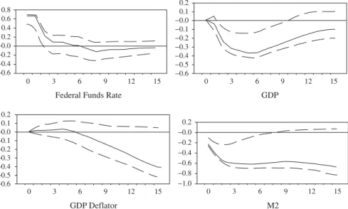
Thus, simple correlations of interest rates (or the money supply) on output or other real variables cannot be used as evidence of non-neutralities. The direction of causality could well go, fully or in part, from movements in the real variable (resulting from nonmonetary forces) to the monetary variable. Over the years, a large literature has developed seeking to answer such questions while avoiding the pitfalls of a simple analysis of comovements. The main challenge facing that literature lies in identifying changes in policy that could be interpreted as autonomous, i.e., not the result of the central bank’s response to movements in other variables. While alternative approaches have been pursued in order to meet that challenge, much of the recent literature has relied on time series econometrics techniques and, in particular, on structural (or identified) vector autoregressions. The evidence displayed in figure 1.1, taken from Christiano, Eichenbaum, and Evans (1999), is representative of the findings in the recent literature seeking to estimate the effects of exogenous monetary policy shocks.12In the empirical model underlying figure 1.1, monetary policy shocks are identified as the residual from an estimated policy rule followed by the Federal Reserve. That policy rule determines the level of the federal funds rate (taken to be the instrument of monetary policy), as a linear function of its own lagged values, current and lagged values of GDP, the GDP deflator, and an index of commodity prices, as well as the lagged values of some monetary aggregates. Under the assumption that neither GDP nor the two price indexes can respond contemporaneously to a monetary policy shock, the coefficients of the previous policy rule can be estimated consistently with ordinary least squares (OLS), and the fitted residual can be taken as an estimate of the exogenous monetary policy shock. The response over time of any variable of interest to that shock is then given by the estimated coefficients of a regression of the current value of that variable on the current and lagged values of the fitted residual from the first-stage regression.
Figure 1.1 shows the dynamic responses of the federal funds rate, (log) GDP, (log) GDP deflator, and the money supply (measured by M2) to an exogenous tightening of monetary policy. The solid line represents the estimated response, with the dashed lines capturing the corresponding 95 percent confidence interval. The scale on the horizontal axis measures the number of quarters after the initial shock. Note that the path of the funds rate itself, depicted in the top left graph, shows an initial increase of about 75 basis points, followed by a gradual return to its original level. In response to that tightening of policy, GDP declines with a characteristic hump-shaped pattern. It reaches a trough after five quarters at a level about 50 basis points below its original level, and then it slowly reverts back to its original level. That estimated response of GDP can be viewed as
12Other references include Sims (1992), Galí (1992), Bernanke and Mihov (1998), and Uhlig (2005).
1.3. Organization of the Book 9
0.8 0.6 0.4 0.2
−0.0
−0.2
−0.4
−0.6
0 3 6
Federal Funds Rate
9 12 15
0.2 0.1
−0.0
−0.2
−0.1
−0.3
−0.4
−0.5
−0.6
0 3 6
GDP
9 12 15
0.2 0.1
−0.0
−0.2
−0.1
−0.3
−0.4
−0.5
−0.6
0 3 6
GDP Deflator
9 12 15 0 3 6 9 12 15
0.2
−0.0
−0.2
−0.4
−0.6
−0.8
−1.0
M2
Figure 1.1 Estimated Dynamic Response to a Monetary Policy Shock
Source: Christiano, Eichenbaum, and Evans (1999).
evidence of sizable and persistent real effects of monetary policy shocks. On the other hand, the (log) GDP deflator displays a flat response for over a year, after which it declines. That estimated sluggish response of prices to the policy tightening is generally interpreted as evidence of substantial price rigidities.13 Finally, note that (log) M2 displays a persistent decline in the face of the rise in the federal funds rate, suggesting that the Fed needs to reduce the amount of money in circulation in order to bring about the increase in the nominal rate. The observed negative comovement between money supply and nominal interest rates is known asliquidity effect. As will be discussed in chapter 2, that liquidity effect appears at odds with the predictions of a classical monetary model.
Having discussed the empirical evidence in support of the key assumptions underlying the New Keynesian framework, this introductory chapter ends with a brief description of the organization of the remaining chapters.
1.3 Organization of the Book
The book is organized into eight chapters, including this introduction. Chapters 2 through 7 progressively develop a unified framework, with new elements being incorporated in each chapter. Throughout the book, the references in the main text are kept to a minimum, and a section is added to the end of each chapter with
13Also, note that expected inflation hardly changes for several quarters and then declines. Combined
10 1. Introduction
a discussion of the literature, including references to the key papers underlying the results presented in the chapter. In addition, each chapter contains a list of suggested exercises related to the material covered in the chapter.
Next, the content of each chapter is briefly described.
Chapter 2 introduces the assumptions on preferences and technology that will be used in most of the remaining chapters. The economy’s equilibrium is determined and analyzed under the assumption of perfect competition in all markets and fully flexible prices and wages. Those assumptions define what is labeled as the classical monetary economy, which is characterized by neutrality of monetary policy and efficiency of the equilibrium allocation. In particular, the specification of monetary policy is shown to play a role only for the determination of nominal variables.
In the baseline model used in the first part of chapter 2, as in the rest of the book, money’s role is limited to being the unit of account, i.e., the unit in terms of which prices of goods, labor services, and financial assets are quoted. Its potential role as a store of value (and hence as an asset in agents’ portfolios), or as a medium of exchange, is ignored. As a result, there is generally no need to specify a money demand function, unless monetary policy itself is specified in terms of a monetary aggregate, in which case a simple log-linear money demand schedule is postulated. The second part of chapter 2, however, generates a motive to hold money by introducing real balances as an argument of the household’s utility function, and examines its implications under the alternative assumptions of separability and nonseparability of real balances. In the latter case, in particular, the result of monetary policy neutrality is shown to break down, even in the absence of nominal rigidities. The resulting non-neutralities, however, are shown to be of limited interest empirically.
Chapter 3 introduces the basic New Keynesian model, by adding product differ-entiation, monopolistic competition, and staggered price setting to the framework developed in chapter 2. Labor markets are still assumed to be competitive. The solution is derived to the optimal price-setting problem of a firm in that environ-ment with the resulting inflation dynamics. The log–linearization of the optimality conditions of households and firms, combined with some market clearing condi-tions, leads to the canonical representation of the model’s equilibrium, which includes the New Keynesian Phillips curve, a dynamic IS equation and a descrip-tion of monetary policy. Two variables play a central role in the equilibrium dynamics: the output gap and the natural rate of interest. The presence of sticky prices is shown to make monetary policy non-neutral. This is illustrated by ana-lyzing the economy’s response to two types of shocks: an exogenous monetary policy shock and a technology shock.
1.3. Organization of the Book 11
level (strict inflation targeting) and alternative ways in which that policy can be implemented are discussed (optimal interest rate rules). There follows a discussion of the likely practical difficulties in the implementation of the optimal policy, which motivates the introduction and analysis of simple monetary policy rules, i.e., rules that can be implemented with little or no knowledge of the economy’s structure and/or realization of shocks. A welfare-based loss function that can be used for the evaluation and comparison of those rules is then derived and applied to two simple rules: a Taylor rule and a constant money growth rule.
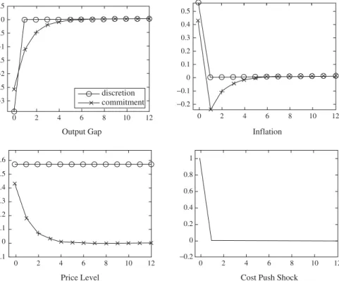
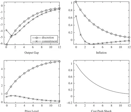
A common criticism of the analysis of optimal monetary policy contained in chapter 4 is the absence of a conflict between inflation stabilization and output gap stabilization in the basic New Keynesian model. In chapter 5 that criticism is addressed by appending an exogenous additive shock to the New Keynesian Phillips curve, thus generating a meaningful policy tradeoff. In that context, and following the analysis in Clarida, Galí, and Gertler (1999), the optimal mone-tary policy under the alternative assumptions of discretion and commitment is discussed, emphasizing the key role played by the forward-looking nature of inflation as a source of the gains from commitment.
Chapter 6 extends the basic New Keynesian framework by introducing imper-fect competition and staggered nominal wage setting in labor markets, in co-existence with staggered price setting and modelled in an analogous way, fol-lowing the work of Erceg, Henderson, and Levin (2000). The presence of sticky nominal wages and the consequent variations in wage markups render a policy aimed at fully stabilizing price inflation as suboptimal. The reason is that fluctu-ations in wage inflation, in addition to varifluctu-ations in price inflation and the output gap, generate a resource misallocation and a consequent welfare loss. Thus, the optimal policy is one that seeks to strike the right balance between stabilization of those three variables. For a broad range of parameters, however, the optimal policy can be well approximated by a rule that stabilizes a weighted average of price and wage inflation, where the proper weights are a function of the relative stickiness of prices and wages.
12 1. Introduction
Finally, chapter 8 reviews some of the general lessons that can be drawn from the previous chapters. In doing so, the focus is on two key insights generated by the new framework, namely, the key role of expectations in shaping the effects of monetary policy, and the importance of the natural levels of output and the interest rate for the design of monetary policy. Chapter 8 ends by describing briefly some of the extensions of the basic New Keynesian model that have not been covered in the book, and by discussing some of the recent developments in the literature.
References
Akerlof, George, and Janet Yellen (1985): “A Near-Rational Model of the Business Cycle with Wage and Price Inertia,”Quarterly Journal of Economics100, 823–838.
Ball, Laurence, and David H. Romer (1990): “Real Rigidities and the Nonneutrality of Money,”Review of Economic Studies57, 183–203.
Basu, Susanto, John Fernald, and Miles Kimball (2006): “Are Technology Improvements Contractionary?”American Economic Review96, no. 5, 1418–1448.
Bayoumi, Tam (2004): “GEM: A New International Macroeconomic Model,”IMF
Occa-sional Paperno. 239.
Bernanke, Ben S., and Ilian Mihov (1998): “Measuring Monetary Policy,”Quarterly Journal of Economics113, no. 3, 869–902.
Bewley, Truman F. (1999):Why Wages Don’t Fall during a Recession?, Harvard University Press, Cambridge, MA.
Bils, Mark, and Peter J. Klenow (2004): “Some Evidence on the Importance of Sticky Prices,”
Journal of Political Economy112, no. 5, 947–985.
Blanchard, Olivier J., and Nobuhiro Kiyotaki (1987): “Monopolistic Competition and the Effects of Aggregate Demand,”American Economic Review77, no. 4, 647–666. Blinder, Alan S., Elie R. D. Canetti, David E. Lebow, and Jeremy B. Rudd (1998):
Ask-ing about Prices: A New Approach to UnderstandAsk-ing Price Stickiness, Russell Sage Foundation, New York.
Cecchetti, Stephen G. (1986): “The Frequency of Price Adjustment: A Study of Newsstand Prices of Magazines,”Journal of Econometrics31, no. 3, 255–274.
Christiano, Lawrence J., Martin Eichenbaum, and Charles L. Evans (1999): “Monetary Policy Shocks: What Have We Learned and to What End?” in J. B. Taylor and M. Woodford (eds.),
Handbook of Macroeconomics1A, Elsevier Science, Amsterdam, 65–148.
Christiano, Lawrence J., Martin Eichenbaum, and Robert Vigfusson (2003): “What Happens After a Technology Shock?” NBER WP#9819.
Clarida, Richard, Jordi Galí, and Mark Gertler (1999): “ The Science of Monetary Policy: A New Keynesian Perspective,”Journal of Economic Literature37, 1661–1707.
Coenen, Günter, Peter McAdam, and Roland Straub (2006): “ Tax Reform and Labour Market Performance in the Euro Area: A Simulation-Based Analysis Using the New Area-Wide Model,”Journal of Economic Dynamics and Control, forthcoming.
Cooley, Thomas F., and Gary D. Hansen (1989): “Inflation Tax in a Real Business Cycle Model,”American Economic Review79, no. 4, 733–748.
References 13
(2006): “Price Changes in the Euro Area and the United States: Some Facts from Individual Consumer Price Data,”Journal of Economic Perspectives20, no. 2, 171–192.
Dickens, William T., Lorenz Goette, Erica L. Groshen, Steinar Holden, Julian Messina, Mark E. Schweitzer, Jarkko Turunen, and Melanie E. Ward (2007): “How Wages Change: Micro Evidence from the International Wage Flexibility Project,” Journal of Economic Perspectives21, no. 2, 195–214.
Edge, Rochelle M., Michael T. Kiley, and Jean-Philippe Laforte (2007): “Documentation of the Research and Statistics Division’s Estimated DSGE Model of the U.S. Economy: 2006 Version,” Federal Reserve Board, Finance and Economics Discussion Series, no. 2007-52. Erceg, Christopher J., Luca Guerrieri, and Christopher Gust (2006): “SIGMA: A New Open Economy Model for Policy Analysis,”International Journal of Central Banking2, no. 1, 1–50.
Erceg, Christopher J., Dale W. Henderson, and Andrew T. Levin (2000): “Optimal Monetary Policy with Staggered Wage and Price Contracts,”Journal of Monetary Economics46, no. 2, 281–314.
Fabiani, Silvia, Martine Druant, Ignacio Hernando, Claudia Kwapil, Bettina Landau, Claire Loupias, Fernando Martins, Thomas Y. Matha, Roberto Sabbatini, Harald Stahl, and Ad. C. J. Stokman (2005): “ The Pricing Behavior of Firms in the Euro Area: New Survey Evidence,”ECB Working Paperno. 535.
Fischer, Stanley (1977): “Long-Term Contracts, Rational Expectations, and the Optimal Money Supply,”Journal of Political Economy85, no. 1, 191–206.
Fisher, Jonas D. M. (2006): “ The Dynamic Effects of Neutral and Investment-Specific Technology Shocks,”Journal of Political Economy114, no. 3, 413–451.
Friedman, Milton, and Anna J. Schwartz (1963):A Monetary History of the United States, 1867–1960, Princeton University Press, Princeton, NJ.
Galí, Jordi (1992): “How Well Does the IS-LM Model Fit Postwar U.S. Data?”Quarterly Journal of Economics107, no. 2, 709–738.
Galí, Jordi (1999): “ Technology, Employment, and the Business Cycle: Do Technology Shocks Explain Aggregate Fluctuations?”American Economic Review89, no. 1, 249–271. Galí, Jordi, and Mark Gertler (2007): “Macroeconomic Modeling for Monetary Policy
Evaluation,”Journal of Economic Perspectives, forthcoming.
Galí, Jordi, and Pau Rabanal (2004): “ Technology Shocks and Aggregate Fluctuations: How Well Does the RBC Model Fit Postwar U.S. Data?,”NBER Macroeconomics Annual 2004, MIT Press, Cambridge, MA.
Goodfriend, Marvin, and Robert G. King (1997): “ The New Neoclassical Synthesis and the Role of Monetary Policy,”NBER Macroeconomics Annual 1997, 231–282.
Kashyap, Anil K. (1995): “Sticky Prices: New Evidence from Retail Catalogues,”Quarterly Journal of Economics110, no. 1, 245–274.
Keynes, John Maynard (1936):The General Theory of Employment, Interest and Money,
MacMillan and Co., London.
Kydland, Finn E., and Edward C. Prescott (1982): “ Time to Build and Aggregate Fluctuations,”Econometrica50, no. 6, 1345–1370.
Lucas, Robert E. (1976): “Econometric Policy Evaluation: A Critique,”Carnegie–Rochester Conference Series on Public Policy1, 19–46.
14 1. Introduction
Nakamura, Emi, and Jon Steinsson (2006): “Five Facts about Prices: A Reevaluation of Menu Costs Models,” Harvard University Press, Cambridge, MA.
Peersman, Gert, and Frank Smets (2003): “ The Monetary Transmission Mechanism in the Euro Area: More Evidence from VAR Analysis,” in Angeloni et al. (eds.),Monetary Policy Transmission in the Euro Area,Cambridge University Press, New York.
Prescott, Edward C. (1986): “ Theory Ahead of Business Cycle Measurement,”Quarterly Review10, 9–22, Federal Reserve Bank of Minneapolis, Minneapolis, MN.
Romer, Christina, and David Romer (1989): “Does Monetary Policy Matter? A New Test in the Spirit of Friedman and Schwartz,”NBER Macroeconomics Annual4, 121–170. Sims, Christopher (1980): “Macroeconomics and Reality,”Econometrica48, no. 1, 1–48. Sims, Christopher (1992): “Interpreting the Macroeconomic Time Series Facts: The Effects
of Monetary Policy,”European Economic Review36, 975–1011.
Smets, Frank, and Raf Wouters (2003): “An Estimated Dynamic Stochastic General Equilib-rium Model of the Euro Area,”Journal of the European Economic Association1, no. 5, 1123–1175.
Taylor, John B. (1980): “Aggregate Dynamics and Staggered Contracts,”Journal of Political Economy88, no. 1, 1–24.
Taylor, John B. (1999): “Staggered Price and Wage Setting in Macroeconomics,” in J. B. Taylor and M. Woodford (eds.), Handbook of Macroeconomics, chap. 15, 1341–1397, Elsevier, New York.
Uhlig, Harald (2005): “What Are the Effects of Monetary Policy on Output? Results from an Anostic Identification Procedure,”Journal of Monetary Economics52, no. 2, 381–419. Walsh, Carl E. (2003):Monetary Theory and Policy, Second Edition, MIT Press, Boston,
MA.
2
A Classical Monetary Model
This chapter presents a simple model of a classical monetary economy, featuring perfect competition and fully flexible prices in all markets. As stressed below, many of the predictions of that classical economy are strongly at odds with the evidence reviewed in chapter 1. That notwithstanding, the analysis of the classical economy provides a benchmark that will be useful in subsequent chapters when some of its strong assumptions are relaxed. It also allows for the introduction of some notation, as well as assumptions on preferences and technology that are used in the remainder of the book.
Following much of the recent literature, the baseline classical model developed here attaches a very limited role to money. Thus, in the first four sections of this chapter, the only explicit role played by money is to serve as a unit of account. In that case, and as shown below, whenever monetary policy is specified in terms of an interest rate rule, no reference whatsoever is made to the quantity of money in circulation in order to determine the economy’s equilibrium. When the speci-fication of monetary policy involves the money supply, a “conventional” money demand equation is postulated in order to close the model without taking a stand on its microfoundations. In section 2.5, an explicit role for money is introduced, beyond that of serving as a unit of account. In particular, a model is analyzed in which real balances are assumed to generate utility to households, and the impli-cations for monetary policy of alternative assumptions on the properties of that utility function are explored.
16 2. A Classical Monetary Model
2.1 Households
The representative household seeks to maximize the objective function
E0
∞
t=0
βtU (Ct, Nt) (1)
where Ct is the quantity consumed of the single good, and Nt denotes hours of work or employment.1The period utilityU (Ct, Nt)is assumed to be contin-uous and twice differentiable, withUc,t≡∂U (C∂Ct,Nt)
t >0,Ucc,t≡
∂2U (Ct,Nt) ∂Ct2 ≤0,
Un,t≡∂U (C∂Nt,Nt)
t ≤0, andUnn,t≡
∂2U (Ct,Nt)
∂Nt2 ≤0. In words, the marginal utility of consumptionUc,tis assumed to be positive and nonincreasing, while the marginal disutility of labor,−Un,t, is positive and nondecreasing.
Maximization of (1) is subject to a sequence of flow budget constraints given by
PtCt+QtBt≤Bt−1+Wt Nt−Tt (2) fort=0,1,2, . . . Ptis the price of the consumption good.Wtdenotes the nominal wage,Btrepresents the quantity of one-period, nominally riskless discount bonds purchased in periodt and maturing in period t+1. Each bond pays one unit of money at maturity and its price is Qt. Tt represents lump-sum additions or subtractions to period income (e.g., lump-sum taxes, dividends, etc.), expressed in nominal terms. When solving the problem above, the household is assumed to take as given the price of the good, the wage, and the price of bonds.
In addition to (2), it is assumed that the household is subject to a solvency constraint that prevents it from engaging in Ponzi-type schemes. The following constraint
lim
T→∞Et{BT} ≥0 (3)
for alltis sufficient for our purposes.
2.1.1 Optimal Consumption and Labor Supply
The optimality conditions implied by the maximization of (1) subject to (2) are given by
−Un,t
Uc,t =
Wt
Pt
(4)
Qt=β Et
Uc,t+1
Uc,t
Pt
Pt+1
(5)
fort=0,1,2, . . ..
1Note thatN
2.1. Households 17
The previous optimality conditions can be derived using a simple variational argument. Let us first consider the impact on utility of a small departure, in period
t, from the household’s optimal plan. That departure consists of an increase in consumption dCt and an increase in hours dNt, while keeping the remaining variables unchanged (including consumption and hours in other periods). If the household was following an optimal plan to begin with, it must be the case that
Uc,t dCt+Un,tdNt=0
for any pair(dCt, dNt)satisfying the budget constraint, i.e.,
PtdCt=WtdNt
for otherwise it would be possible to raise utility by increasing (or decreasing) consumption and hours, thus contradicting the assumption that the household is on an optimal plan. Note that by combining both equations the optimality condition (4) is obtained.
Similarly, consider the impact on expected utility as of timet of a reallocation of consumption between periodst andt+1, while keeping consumption in any period other thantandt+1, and hours worked (in all periods) unchanged. If the household is optimizing, it must be the case that
Uc,t dCt+β Et{Uc,t+1dCt+1} =0
for any pair(dCt, dCt+1)satisfying
Pt+1dCt+1= −
Pt
Qt
dCt
where the latter equation determines the increase in consumption expenditures in periodt+1 made possible by the additional savings−PtdCtallocated into one-period bonds. Combining the two previous equations yields the intertemporal optimality condition (5).
Much of what follows, assumes that the period utility takes the form
U (Ct, Nt)=
C1−σ t 1−σ −
Nt1+ϕ 1+ϕ.
The consumer’s optimality conditions (4) and (5) thus become
Wt
Pt
=CtσNtϕ (6)
Qt=β Et
Ct+1
Ct
−σ
Pt
Pt+1
18 2. A Classical Monetary Model
Note, for future reference, that equation (6) can be rewritten in log-linear form as
wt−pt=σ ct+ϕ nt (8)
where lowercase letters denote the natural logs of the corresponding variable (i.e.,
xt≡logXt). The previous condition can be interpreted as a competitive labor supply schedule, determining the quantity of labor supplied as a function of the real wage, given the marginal utility of consumption (which under the assumptions is a function of consumption only).
As shown in appendix 2.1, a log-linear approximation of (7) around a steady state with constant rates of inflation and consumption growth is given by
ct=Et{ct+1} − 1
σ (it−Et{πt+1} −ρ) (9)
whereit≡ −logQt,ρ≡ −logβand whereπt+1≡pt+1−ptis the rate of infla-tion betweentandt+1 (having definedpt≡logPt). Notice thatit corresponds to the log of the gross yield on the one-period bond; henceforth, it is referred to as thenominal interest rate.2 Similarly,ρ can be interpreted as the household’s discount rate.
While the previous framework does not explicitly introduce a motive for holding money balances, in some cases it will be convenient to postulate a demand for real balances with a log-linear form given by (up to an additive constant)
mt−pt=yt−η it (10)
whereη≥0 denotes the interest semi-elasticity of money demand.
A money demand equation similar to (10) can be derived under a variety of assumptions. For instance, in section 2.5 it is derived as an optimality condition for the household when money balances yield utility.
2.2 Firms
A representative firm is assumed whose technology is described by a production function given by
Yt=AtNt1−α (11)
whereAtrepresents the level of technology, andat≡logAtevolves exogenously according to some stochastic process.
Each period the firm maximizes profits
Pt Yt−WtNt (12)
subject to (11), taking the price and wage as given.
2The yield on the one period bond is defined byQ
2.3. Equilibrium 19
Maximization of (12) subject to (11) yields the optimality condition
Wt
Pt
=(1−α) AtNt−α (13)
i.e., the firm hires labor up to the point where its marginal product equals the real wage. Equivalently, the marginal cost Wt
(1−α)AtNt−α must be equated to the pricePt. In log-linear terms,
wt−pt=at−α nt+log(1−α) (14)
which can be interpreted as labor demand schedule, mapping the real wage into the quantity of labor demanded, given the level of technology.
2.3 Equilibrium
The baseline model abstracts from aggregate demand components like investment, government purchases, or net exports. Accordingly, the goods market clearing condition is given by
yt=ct (15)
i.e., all output must be consumed.
By combining the optimality conditions of households and firms with (15) and the log-linear aggregate production relationship
yt=at+(1−α) nt (16)
the equilibrium levels of employment and output are determined as a function of the level of technology
nt=ψnaat+ϑn (17)
yt=ψyaat+ϑy (18)
where ψna≡ σ (1−1α)−+σϕ+α, ϑn≡ log(1− α)
σ (1−α)+ϕ+α, ψya≡ 1+ϕ
σ (1−α)+ϕ+α, and
ϑy≡(1−α)ϑn.
Furthermore, given the equilibrium process for output, (9) can be used to determine the implied real interest rate,rt≡it−Et{πt+1}, as
rt=ρ+σ Et{yt+1}
=ρ+σ ψyaEt{at+1}. (19) Finally, the equilibrium real wageωt≡wt−ptis given by
ωt=at−α nt+log(1−α) (20)
=ψωa at+ϑω
whereψωa≡ σ+ϕ
σ (1−α)+ϕ+α andϑω≡
20 2. A Classical Monetary Model
Notice that the equilibrium dynamics of employment, output, and the real interest rate are determinedindependently of monetary policy. In other words, monetary policy is neutral with respect to those real variables. In the simple model, output and employment fluctuate in response to variations in technology, which is assumed to be the only real driving force.3 In particular, output always rises in the face of a productivity increase, with the size of the increase being given byψya>0. The same is true for the real wage. On the other hand, the sign of the employment is ambiguous, depending on whetherσ(which measures the strength of the wealth effect of labor supply) is larger or smaller than one. Whenσ <1, the substitution effect on labor supply resulting from a higher real wage dominates the negative effect caused by a smaller marginal utility of consumption, leading to an increase in employment. The converse is true wheneverσ >1. When the utility of consumption is logarithmic (σ=1), employment remains unchanged in the face of technology variations, for substitution and wealth effects exactly cancel one another. Finally, the response of the real interest rate depends critically on the time series properties of technology. If the current improvement in technology is transitory so thatEt{at+1}< at, then the real rate will go down. Otherwise, if technology is expected to keep improving, thenEt{at+1}> at and the real rate will increase with a rise inat.
What about nominal variables, like inflation or the nominal interest rate? Not surprisingly, and in contrast with real variables, their equilibrium behavior cannot be determined uniquely by real forces. Instead, it requires the specification of how monetary policy is conducted. Several monetary policy rules and their implied outcomes will be considered next.
2.4 Monetary Policy and Price Level Determination
Let us start by examining the implications of some interest rate rules. Rules that involve monetary aggregates will be introduced later. All cases will make use of the Fisherian equation
it=Et{πt+1} +rt (21)
that implies that the nominal rate adjusts one for one with expected inflation, given a real interest rate that is determined exclusively by real factors, as in (19).
2.4.1 An Exogenous Path for the Nominal Interest Rate
Let us first consider the case of the nominal interest rate following anexogenous stationary process{it}. Without loss of generality, assume thatit has meanρ,
3It would be straightforward to introduce other real driving forces like variations in government
2.4. Monetary Policy and Price Level Determination 21
which is consistent with a steady state with zero inflation and no secular growth. Notice that a particular case of this rule corresponds to a constant interest rate
it=i=ρ for allt. Using (21), write
Et{πt+1} =it−rt
where, as discussed above,rtis determined independently of the monetary policy rule.
Note that expected inflation is pinned down by the previous equation but actual inflation is not. Because there is no other condition that can be used to determine inflation, it follows that any path for the price level that satisfies
pt+1=pt+it−rt+ξt+1
is consistent with equilibrium, whereξt+1is a shock, possibly unrelated to eco-nomic fundamentals, satisfying Et{ξt+1} =0 for all t. Such shocks are often referred to in the literature as sunspot shocks. An equilibrium in which such nonfundamental factors may cause fluctuations in one or more variables is referred to as anindeterminate equilibrium. The example above shows how an exogenous nominal interest rate leads toprice level indeterminacy.
Notice that when (10) is operative the equilibrium path for the money supply (which is endogenous under the present policy regime) is given by
mt=pt+yt−η it.
Hence, the money supply will inherit the indeterminacy ofpt. The same will be true of the nominal wage (which, in logs, equals the real wage, which is determined by (20) plus the price level, which is indeterminate).
2.4.2 A Simple Inflation-Based Interest Rate Rule
Suppose that the central bank adjusts the nominal interest rate according to the rule
it=ρ+φπ πt
whereφπ ≥0.
Combining the previous rule with the Fisherian equation (21) yields
φπ πt=Et{πt+1} +rt (22)
22 2. A Classical Monetary Model
If φπ>1, the previous difference equation has only one stationary solution, i.e., a solution that remains in a neighborhood of the steady state. That solution can be obtained by solving (22) forward, which yields
πt=
∞
k=0
φ−π(k+1)Et{rt+k}. (23)
The previous equation fully determines inflation (and, hence, the price level) as a function of the path of the real interest rate, which in turn is a function of fundamentals, as shown in (19). Consider, for the sake of illustration, the case in which technology follows the stationary AR(1) process
at=ρaat−1+εat
whereρa∈ [0,1). Then, (19) impliesrt= −σ ψya(1−ρa) at, which combined with (23) yields the following expression for equilibrium inflation
πt= −
σ ψya(1−ρa)
φπ−ρa
at.
Note that a central bank following a rule of the form considered here can influ-ence the degree of inflation volatility by choosing the size ofφπ. The larger is the latter parameter the smaller will be the impact of the real shock on inflation.
On the other hand, ifφπ<1, the stationary solutions to (22) take the form
πt+1=φπ πt−rt+ξt+1 (24)
where {ξt} is, again, an arbitrary sequence of shocks, possibly unrelated to fundamentals, satisfyingEt{ξt+1} =0 for allt.
Accordingly, any process {πt}satisfying (24) is consistent with equilibrium, while remaining in a neighborhood of the steady state. So, as in the case of an exogenous nominal rate, the price level (and, hence, inflation and the nominal rate) are not determined uniquely when the interest rate rule implies a weak response of the nominal rate to changes in inflation. More specifically, the condition for a determinate price level,φπ>1, requires that the central bank adjust nominal interest rates more than one for one in response to any change in inflation, a property known as theTaylor principle. The previous result can be viewed as a particular instance of the need to satisfy the Taylor principle in order for an interest rate rule to bring about a determinate equilibrium.
2.4.3 An Exogenous Path for the Money Supply
2.4. Monetary Policy and Price Level Determination 23
equation for the price level can be derived as
pt=
η
1+η
Et{pt+1} +
1 1+η
mt+ut
whereut≡(1+η)−1(η rt−yt)evolves independently of{mt}. Assumingη >0 and solving forward obtains
pt= 1 1+η
∞
k=0
η
1+η
k
Et{mt+k} +ut
whereut≡ ∞k=0(1+ηη)kE
t{ut+k}is, again, independent of monetary policy. Equivalently, the previous expression can be rewritten in terms of expected future growth rate of money as
pt=mt+
∞
k=1
η
1+η
k
Et{mt+k} +ut. (25)
Hence, an arbitrary exogenous path for the money supply always determines the price level uniquely. Given the price level, as determined above, (10) can be used to solve for the nominal interest rate
it=η−1[yt−(mt−pt)]
=η−1 ∞
k=1
η
1+η
k
Et{mt+k} +u t
whereu t ≡η−1(u
t+yt)is independent of monetary policy.
For example, consider the case in which money growth follows the AR(1) process
mt=ρmmt−1+εmt .
For simplicity, assume the absence of real shocks, thus implying a constant output and a constant real rate. Without loss of generality, setrt=yt=0 for allt. Then, it follows from (25) that
pt=mt+
ηρm 1+η(1−ρm)
mt.
Hence, in response to an exogenous monetary policy shock, and as long as
24 2. A Classical Monetary Model
The nominal interest rate is in turn given by
it=
ρm 1+η(1−ρm)
mt
i.e., in response to an expansion of the money supply, and as long asρm>0, the nominal interest rate is predicted to go up. In other words, the model implies the absence of a liquidity effect, in contrast with the evidence discussed in chapter 1.
2.4.4 Optimal Monetary Policy
The analysis of the baseline classical economy above has shown that while real variables are independent of monetary policy, the latter can have important impli-cations for the behavior of nominal variables and, in particular, of prices. Yet, and given that the household’s utility is a function of consumption and hours only— two real variables that are invariant to the way monetary policy is conducted—it follows that there is no policy rule that is better than any other. Thus, in the clas-sical model above, a policy that generates large fluctuations in inflation and other nominal variables (perhaps as a consequence of following a policy rule that does not guarantee a unique equilibrium for those variables) is no less desirable than one that succeeds in stabilizing prices in the face of the same shocks.
The previous result, which is clearly extreme and empirically unappealing, can be overcome once versions of the classical monetary model are considered in which a motive to keep part of a household’s wealth in the form of monetary assets is introduced explicitly. Section 2.5 discusses one such model in which real balances are assumed to yield utility.
The overall assessment of the classical monetary model as a framework to understand the joint behavior of nominal and real variables and their con-nection to monetary policy cannot be positive. The model cannot explain the observed real effects of monetary policy on real variables. Its predictions regard-ing the response of the price level, the nominal rate, and the money supply to exogenous monetary policy shocks are also in conflict with the empirical evi-dence. Those empirical failures are the main motivation behind the introduction of nominal frictions in otherwise similar models, a task that will be undertaken in chapter 3.
2.5 Money in the Utility Function
In the model developed in the previous sections, and in much of the recent mone-tary literature, the only role played by money is to serve as a numéraire, i.e., a unit of account in which prices, wages, and securities’ payoffs are stated.4Economies
4Readers not interested in this extension may skip this section and proceed to section 2.6 without any
2.5. Money in the Utility Function 25
with that characteristic are often referred to ascashless economies. Whenever a simple log-linear money demand function was postulated, it was done in an ad-hoc manner without an explicit justification for why agents would want to hold an asset that is dominated in return by bonds while having identical risk properties. Even though in the analysis of subsequent chapters the assumption of a cashless economy is held, it is useful to understand how the basic framework can incorpo-rate a role for money other than that of a unit of account and, in particular, how it can generate a demand for money. The discussion in this section focuses on models that achieve the previous objective by assuming that real balances are an argument of the utility function.
The introduction of money in the utility function requires modifying the household’s problem in two ways. First, preferences are now given by
E0
∞
t=0
βtU
Ct,
Mt
Pt
, Nt
(26)
whereMt denotes holdings of money in periodt. Assume that period utility is increasing and concave in real balancesMt/Pt. Second, the flow budget constraint incorporates monetary holdings explicitly, taking the form
PtCt+Qt Bt+Mt≤Bt−1+Mt−1+Wt Nt−Tt.
By lettingAt≡Bt−1+Mt−1denote total financial wealth at the beginning of the periodt(i.e., before consumption and portfolio decisions are made), the previous flow budget constraint can be rewritten as
PtCt+QtAt+1+(1−Qt)Mt≤At+Wt Nt−Tt (27)
with the solvency constraint now taking the form
limT→∞Et{AT} ≥0, for allt.
The previous representation of the budget constraint can be thought of as equiv-alent to that of an economy in which all financial assets (represented byAt) yield a gross nominal returnQ−t1(=exp{it}), and where agents can purchase the utility-yielding “services” of money balances at a unit price(1−Qt)=1−exp{−it}
it. Thus, the implicit price for money services roughly corresponds to the nominal interest rate, which in turn is the opportunity cost of holding one’s financial wealth in terms of monetary assets, instead of interest-bearing bonds.