Dynamic obstacles avoidance algorithms for unmanned ground vehicles
256
0
0
Texto completo
(2)
(3)
(4) ESCUELA DE DOCTORADO Servicio de Estudios Oficiales de Posgrado. DILIGENCIA DE DEPÓSITO DE TESIS.. EDUARDO JOSÉ MOLINOS VICENTE Comprobado que el expediente académico de D./Dª ____________________________________________ reúne los requisitos exigidos para la presentación de la Tesis, de acuerdo a la normativa vigente, y habiendo presentado la misma en formato: soporte electrónico. impreso en papel, para el depósito de la. 252 misma, en el Servicio de Estudios Oficiales de Posgrado, con el nº de páginas: __________ se procede, con fecha de hoy a registrar el depósito de la tesis.. 17 26 de ___________________ ABRIL Alcalá de Henares a _____ de 20_____. Rosa Carrillo Salas Fdo. El Funcionario.
(5) Universidad de Alcalá PhD. Program in Electronics: Advanced Electronic Systems. Intelligent Systems. Dynamic Obstacles Avoidance Algorithms for Unmanned Ground Vehicles PhD. Thesis Presented by Eduardo José Molinos Vicente. 2017.
(6)
(7) Universidad de Alcalá PhD. Program in Electronics: Advanced Electronic Systems. Intelligent Systems. Dynamic Obstacles Avoidance Algorithms for Unmanned Ground Vehicles PhD. Thesis Presented by Eduardo José Molinos Vicente Advisor Dr. Manuel Ocaña Miguel. Alcalá de Henares, 2017.
(8)
(9)
(10)
(11)
(12)
(13) “Which is the longest path? Any path is the longest when the feet go and the heart doesn’t” - Alejandro Jodorowsky.
(14)
(15) Agradecimientos Tras mucho tiempo y sacrificio, pero también muchos momentos buenos y constructivos me encuentro escribiendo estos agradecimientos. Al final estas lı́neas resumen unos cuantos años de mi vida y una etapa de la que me llevo muchos gratos recuerdos. Para empezar quiero agradecer a mi familia más cercana, porque ellos son los que más me han apoyado y han tenido que soportar el estrés y las tensiones que se derivan de la elaboración de una tesis. Desde luego sin ellos hubiera sido imposible. Para continuar tengo que dar las gracias a mi tutor, Manuel. Primero, por confiar en mı́ cuando aún era un estudiante de segundo de carrera. Lo que empezó con un pequeño proyecto llevando la página web para complementar mis estudios ha terminado con muchos años de trabajo juntos. Y segundo, por todo el apoyo y el tiempo que me ha dedicado en esos años. Siguiendo en orden de importancia quiero dar las gracias a toda la gente del Robe-Isis. Ángel por aguantarme todos los dı́as, por los pocos (seguro que aún queda alguno más), viajes y momentos compartidos. Noelia que llevamos compartiendo pupitres (¡y al final hasta barrio!) más de una decada. Fer por todas las risas que nos hemos echado. Nacho por todo el tiempo compartido y la ayuda que ha proporcionado en esta tesis. Rober por surtirnos de jugosos pasteles siempre que la ocasión lo requerı́a. A los chicos del Isis/Invett por tantos desayunos (Raúl, Carlos, Mario, Rubén, Javi, Carlota). También a todos los que han pasado por aquı́ estos años: Jorge, Javi, Balki, Augusto, Hugo. Y por último para los alumnos de TFG que terminaron siendo compañeros: Raúl, Rocı́o, Fran, Guillermo, Carlos (y seguro que para cuando este libro salga a la luz, Adrián, Alejandro,.
(16) 12 Adolfo, Eduardo y David). Gracias también a los profesores (Manuel, Dani, Elena, Carlos, Luismi) y los alumnos con los que he podido compartir labores docentes. Cada hora de clase ha sido una experiencia enriquecedora. No quiero olvidarme tampoco de dar las gracias al fabuloso equipo con el que coincidı́ en Edimburgo. Ir a un paı́s que no conoces no suele ser nada fácil, pero desde luego con un grupo ası́ lo fue. Ası́ que gracias a todos, especialmente a Sethu, Vlad, Jose y Yimming. No puedo terminar estos agradecimientos sin pedir disculpas si me dejo a alguien. Son muchos años en la universidad entre unas cosas y otras y mi memoria cada vez es peor. Ası́ que si estas leyendo esto y crees que mereces estar aquı́, ¡gracias a ti también!.
(17) Resumen En las últimas décadas, los vehı́culos terrestres no tripulados (UGVs) están siendo cada vez más empleados como robots de servicios. A diferencia de los robots industriales, situados en posiciones fijas y controladas, estos han de trabajar en entornos dinámicos, compartiendo su espacio con otros vehı́culos y personas. Los UGVs han de ser capaces de desplazarse sin colisionar con ningún obstáculo, de tal manera que puedan asegurar tanto su integridad como la del entorno. En el estado del arte encontramos algoritmos de navegación autónoma diseñados para UGVs que son capaces de planificar rutas de forma segura con objetos estáticos y trabajando en entornos parcialmente controlados. Sin embargo, cuando estos entornos son dinámicos, se planifican rutas más peligrosas y que a menudo requieren de un mayor consumo de energı́a y recursos, e incluso pueden llegar a bloquear el UGV en un mı́nimo local. En esta tesis, la adaptación de algunos algoritmos disponibles en el estado del arte para trabajar en entornos dinámicos han sido planteados. Estos algoritmos incluyen información temporal tales como los basados en arcos de curvatura (PCVM y DCVM) y los basados en ventanas dinámicas (DW4DO y DW4DOT). Además, se ha propuesto un planificador global basado en Lattice State Planner (DLP) que puede resolver situaciones donde los evitadores de obstáculos reactivos no funcionan. Estos algoritmos han sido validados tanto en simulación como en entornos reales, utilizando distintas plataformas robóticas, entre las que se incluye un robot asistente (RoboShop) diseñado y construido en el marco de esta tesis. Palabras Clave: Navegación autónoma, Evitación de obstáculos.
(18) II dinámicos, Planificación de caminos, Vehı́culos terrestres no tripulados..
(19) Abstract In the recent years, unmanned ground vehicles (UGVs) are being increasingly used as service robots. Unlike industrial robots, which are situated in fixed and controlled positions, UGVs work in dynamic environments, sharing the space with other vehicles and humans. UGVs should being able to move without colliding with any obstacle, assuring its integrity and the environment safety. In the state of the art, navigation algorithms for UGVs are able to plan routes in a safe way, with static obstacles and work in partially controlled environments. However, when the environment is dynamic, the paths planned are more dangerous and often result in more energy and resources consumption, or even can block the UGV in a local minima situation. In this thesis, adaptation of state of the art algorithms for working in dynamic environments has been proposed. These algorithms take into account time information, such as based on curvature arcs (PCVM and DCVM) and based on dynamic window approach (DW4DO and DW4DOT). A global path planning algorithm based in Lattice State Planner (DLP) that can solve situations where an obstacle avoidance algorithm does not work is also proposed. These algorithms have been validated in both simulated and real tests using several robotic platforms, including an assistant robot (RoboShop) that has also been designed and built during this thesis development. KeyWords: Autonomous Navigation, Dynamic Obstacle Avoidance, Path Planning, Unmanned Ground Vehicles..
(20)
(21) Table of Contents Resumen. I. Abstract. III. Table of Contents. V. List of Figures. IX. List of Tables. XV. List of Acronyms 1 Introduction 1.1 Motivation . . . . . . 1.2 Scope of this thesis . 1.3 Proposal . . . . . . . 1.4 Document structure .. XVII. . . . .. 1 1 8 9 10. . . . .. 11 12 15 25 33. 3 Architecture 3.1 Robotics Middlewares . . . . . . . . . . . . . . . . . 3.1.1 ROS . . . . . . . . . . . . . . . . . . . . . . . 3.2 Robotic Platforms . . . . . . . . . . . . . . . . . . .. 35 35 41 46. . . . .. . . . .. 2 State of the Art 2.1 Perception and Mapping 2.2 Local Navigation . . . . 2.3 Global Path Planning . . 2.4 Objectives . . . . . . . .. . . . .. . . . .. V. . . . .. . . . .. . . . .. . . . .. . . . .. . . . .. . . . .. . . . .. . . . .. . . . .. . . . .. . . . .. . . . .. . . . .. . . . .. . . . .. . . . .. . . . .. . . . .. . . . .. . . . .. . . . .. . . . .. . . . .. . . . .. . . . .. . . . .. . . . ..
(22) VI. TABLE OF CONTENTS 3.2.1. 3.3. Commercial Platforms . . . . . . . . . . . . . 3.2.1.1 Pioneer Robots . . . . . . . . . . . . 3.2.1.2 Pioneer 3-DX and Pioneer 3-AT . . . 3.2.1.3 Seekur Jr . . . . . . . . . . . . . . . 3.2.2 Developed Platforms . . . . . . . . . . . . . . 3.2.2.1 PROPINA Platform . . . . . . . . . 3.2.2.2 PROPINA Platform: Mechanical design . . . . . . . . . . . . . . . . . . 3.2.2.3 PROPINA Platform: Electronic design 3.2.2.4 PROPINA Platform: Software . . . 3.2.2.5 Modelling PROPINA in Gazebo . . 3.2.2.6 RoboShop Platform . . . . . . . . . 3.2.2.7 Modelling RoboShop in Gazebo . . . Robotic Platforms Comparison . . . . . . . . . . . .. 4 Development 4.1 Local Mapping . . . . . . . . . . . . . . . . . . 4.2 Algorithms Based on Curvature Arcs . . . . . . 4.2.1 Curvature Velocity Method . . . . . . . 4.2.2 Predicted Curvature Velocity Method . . 4.2.3 Dynamic Curvature Velocity Method . . 4.2.4 Conclusions . . . . . . . . . . . . . . . . 4.3 Dynamic Window based Algorithms . . . . . . . 4.3.1 Dynamic Window for Dynamic Obstacles 4.3.2 Dynamic Window for Dynamic Obstacles 4.3.3 Conclusions . . . . . . . . . . . . . . . . 4.4 Dynamic Lattice Planner . . . . . . . . . . . . . 5 Results 5.1 Simulation Results . . . . . . . . . . 5.1.1 Parameters Sensitivity Studio 5.1.2 Dynamic Obstacle Avoidance 5.1.3 Navigation . . . . . . . . . . . 5.1.4 Global Path Planning . . . . 5.2 Real Robot Experiments . . . . . . . 5.2.1 Dynamic Obstacle Avoidance 5.2.2 Global Path Planning . . . .. . . . . . . . .. . . . . . . . .. . . . . . . . .. . . . . . . . .. . . . . . . . .. . . . . . . . .. 46 47 47 48 49 50 51 52 57 61 64 66 69. . . . . . . . . . . . . . . . . . . . . . . . . Tree . . . . . .. 77 78 92 92 106 107 111 112 113 126 130 131. . . . . . . . .. 141 141 141 151 160 163 172 172 178. . . . . . . . .. . . . . . . . ..
(23) TABLE OF CONTENTS 5.2.3 5.2.4. VII. ABSYNTHE Project . . . . . . . . . . . . . . RoboShop Project . . . . . . . . . . . . . . .. 180 182. 6 Conclusions and Future Work 185 6.1 Main Contributions . . . . . . . . . . . . . . . . . . . 186 6.2 Future Work . . . . . . . . . . . . . . . . . . . . . . . 187 Appendices. 189. A Localisation, Perception and Control Algorithms 191 A.1 Localisation System . . . . . . . . . . . . . . . . . . . 191 A.2 Perception System . . . . . . . . . . . . . . . . . . . 198 A.3 Robot’s Control . . . . . . . . . . . . . . . . . . . . . 200 B Publications Derived from this PhD Dissertation B.1 Journal Publications . . . . . . . . . . . . . . . . . B.2 Conference Publications . . . . . . . . . . . . . . . B.3 Partially Related Publications . . . . . . . . . . . . B.3.1 Journal Publications . . . . . . . . . . . . . B.3.2 Conference Publications . . . . . . . . . . . Bibliography. . . . . .. 205 205 206 207 207 207 209.
(24)
(25) List of Figures 1.1 1.2 1.3 1.4 1.5 1.6 1.7. Assembly line. . . . . . . . . . . . . . . . . . . . . . . Estimated worldwide annual supply of industrial robots Forecast supply of industrial robots . . . . . . . . . . Estimated worldwide annual supply of service robots Forecast supply of service robots for domestic use . . Autonomous Navigation Stages Diagram . . . . . . . DARPA Challenge Autonomous Robots . . . . . . .. 2 2 3 4 4 5 8. 2.1 2.2 2.3 2.4 2.5 2.6 2.7. Topological (left) and metric (right) mapping . . . . Cells Discretisation Techniques. Credits to M. Huber Bug2 Example. Credits to H. Choset . . . . . . . . . VFF Example. Credits to J. Borenstein et al. . . . . VFH Example. Credits to J. Borenstein and Y. Koren DWA Example. Credits to D. Fox et al. . . . . . . . ND scenarios classification. Credits to J. Minguez and L. Montano . . . . . . . . . . . . . . . . . . . . . . . LCM Example. Credits to N. Y. Ko et al. . . . . . . Collision Cone Example. Credits to X. Zhong et al. . TVDW Example. Credits to M.Seder and I.Petrovic . Wavefront Example . . . . . . . . . . . . . . . . . . . Global Potential Field. Local Minima Problem Example Visibility Graph and Voronoi Diagram Example . . . State Lattice Planning Example. Credits to M. Pivtoraiko and A. Kelly . . . . . . . . . . . . . . . . . . Decision Tree Example . . . . . . . . . . . . . . . . . Hybrid A* Example. . . . . . . . . . . . . . . . . . .. 14 15 16 17 18 19. 2.8 2.9 2.10 2.11 2.12 2.13 2.14 2.15 2.16. IX. 20 21 22 23 26 27 28 29 29 32.
(26) X. LIST OF FIGURES 3.1 3.2 3.3 3.4 3.5 3.6 3.7 3.8 3.9 3.10 3.11 3.12 3.13 3.14 3.15 3.16 3.17 3.18 3.19 3.20 3.21 3.22 3.23 3.24 3.25 3.26 4.1 4.2 4.3 4.4 4.5 4.6. Robotics Simulators . . . . . . . . . . . . . . . . . . . ROS architecture example . . . . . . . . . . . . . . . RViz example . . . . . . . . . . . . . . . . . . . . . . RobeSafe Group’s Robots . . . . . . . . . . . . . . . Pioneer 3 Robots . . . . . . . . . . . . . . . . . . . . Seekur Jr: platform and dimensions . . . . . . . . . . PROPINA: design and logo . . . . . . . . . . . . . . Plataforma Robótica Para La Investigación (PROPINA) platform . . . . . . . . . . . . . . . . . . PROPINA: PM10 Motor and gearbox . . . . . . . . . PROPINA: Motor’s Driver and Arduino boards. . . . PROPINA: Wheel encoder RI38 . . . . . . . . . . . . PROPINA: Infrared Sensor . . . . . . . . . . . . . . Infrared Sensor: Transfer function and Polynomial Approximation . . . . . . . . . . . . . . . . . . . . . . . PROPINA: Sonar Range Sensor . . . . . . . . . . . . PROPINA: Software Diagram . . . . . . . . . . . . . Gazebo model of PROPINA . . . . . . . . . . . . . . Gazebo diagram of PROPINA . . . . . . . . . . . . . RoboShop platform . . . . . . . . . . . . . . . . . . . RoboShop Diagram . . . . . . . . . . . . . . . . . . . Hokuyo URG-04LX in Gazebo . . . . . . . . . . . . . Depth Camera sensor in Gazebo . . . . . . . . . . . . Gazebo model of RoboShop . . . . . . . . . . . . . . Gazebo diagram of RoboShop . . . . . . . . . . . . . UMBmark path . . . . . . . . . . . . . . . . . . . . . Comparison of platform’s odometry based on UMBmark Comparison of platform’s odometry on real runs . . .. 39 43 44 47 48 49 50. Local Mapping Example . . . . . . . . . . . . . . . . Local Mapping Example: Current Situation . . . . . Local Mapping Example: Insert Static Obstacles . . . Local Mapping Example: Insert Dynamic Obstacles . Local Mapping Example: Order and Filter Cells (First Time) . . . . . . . . . . . . . . . . . . . . . . . . . . Local Mapping Example: Move the Previous Local Map. 81 82 82 83. 52 53 54 54 55 56 57 58 63 64 65 66 67 68 68 69 71 74 75. 84 85.
(27) LIST OF FIGURES 4.7. XI. 4.13 4.14 4.15 4.16 4.17 4.18 4.19 4.20 4.21 4.22 4.23 4.24 4.25 4.26 4.27 4.28 4.29 4.30 4.31 4.32. Local Mapping Example: Previous Local Map after Raytrace . . . . . . . . . . . . . . . . . . . . . . . . . Local Mapping Example: Add Previous and Current Local Maps . . . . . . . . . . . . . . . . . . . . . . . Local Mapping Example: Order and Filter Cells (Second Time) . . . . . . . . . . . . . . . . . . . . . . . . Obstacle Enlargement Example . . . . . . . . . . . . Local Mapping Example: Enlarge Obstacles . . . . . Local Mapping Example: Order and Filter Cells (Third Time) . . . . . . . . . . . . . . . . . . . . . . Local Mapping Example: Final Map . . . . . . . . . Local Mapping Flowchart . . . . . . . . . . . . . . . CVM: Local Mapping Stage . . . . . . . . . . . . . . CVM: Tangent curvature arcs to obstacles . . . . . . CVM: Curvature Interval contained in the current one CVM: Curvature Interval contains the current one . . CVM: Curvature Interval Overlapped . . . . . . . . . CVM: Curvature Interval Reduction . . . . . . . . . . CVM: Set of curvature arcs . . . . . . . . . . . . . . CVM: Flowchart . . . . . . . . . . . . . . . . . . . . PCVM: Risky Situation . . . . . . . . . . . . . . . . DCVM: Local Mapping Stage . . . . . . . . . . . . . DCVM Diagram . . . . . . . . . . . . . . . . . . . . Dynamic Window Example . . . . . . . . . . . . . . Collision Checking . . . . . . . . . . . . . . . . . . . DW4DO: Flowchart . . . . . . . . . . . . . . . . . . . DW4DOT: Tree building techniques . . . . . . . . . . A* Path Planning Example . . . . . . . . . . . . . . Multilevel Grid Map . . . . . . . . . . . . . . . . . . DLP: Flowchart . . . . . . . . . . . . . . . . . . . . .. 90 91 92 94 96 97 98 99 100 102 105 107 108 111 116 118 126 129 133 135 140. 5.1 5.2 5.3 5.4 5.5 5.6. CVM Parameters Test: Scenario 1 . . . . . CVM Parameters Test: Scenario 2 . . . . . CVM Parameters Test: Scenario 3: Results DW4DO Parameters Test: Scenario 1 . . . DW4DO Parameters Test: Scenario 2 . . . DW4DO Parameters Test: Scenario 3 . . .. 144 145 146 148 149 151. 4.8 4.9 4.10 4.11 4.12. . . . . . .. . . . . . .. . . . . . .. . . . . . .. . . . . . .. . . . . . .. 86 86 87 88 89.
(28) XII 5.7 5.8. LIST OF FIGURES. 5.11 5.12 5.13 5.14 5.15 5.16 5.17 5.18 5.19 5.20 5.21 5.22 5.23 5.24 5.25 5.26 5.27 5.28 5.29 5.30 5.31 5.32 5.33 5.34. Dynamic Obstacle Avoidance: Two obstacles crossing Dynamic Obstacle Avoidance: Corner and Two Obstacles . . . . . . . . . . . . . . . . . . . . . . . . . . Dynamic Obstacle Avoidance: Corner and Two Obstacles Approaching the Robot . . . . . . . . . . . . . Dynamic Obstacle Avoidance: Multiple Obstacles and Moving Obstacle approaching the robot . . . . . . . . Dynamic Obstacle Avoidance: Crossroad . . . . . . . Dynamic Obstacle Avoidance: Lane Changing . . . . Navigation: Scenario 1 . . . . . . . . . . . . . . . . . Navigation: Scenario 2 . . . . . . . . . . . . . . . . . Navigation: Scenario 3 . . . . . . . . . . . . . . . . . A* Weight Function Evaluation: Scenario 1 . . . . . A* Weight Function Evaluation: Scenario 2 . . . . . A* Multi Resolution Test: Scenario 1 . . . . . . . . . A* Multi Resolution Test: Scenario 2 . . . . . . . . . DLP + A* evaluation: Scenario 1 . . . . . . . . . . . DLP + A* evaluation: Scenario 2 . . . . . . . . . . . DLP Lane Example . . . . . . . . . . . . . . . . . . . DLP Semaphore Test . . . . . . . . . . . . . . . . . . DLP Dynamic Obstacle Example . . . . . . . . . . . Dynamic Obstacle Avoidance: Real Scenario 1 . . . . Dynamic Obstacle Avoidance: Real Scenario 2 . . . . Dynamic Obstacle Avoidance: Real Scenario 3 . . . . Dynamic Obstacle Avoidance: Real Scenario 4 . . . . Dynamic Obstacle Avoidance: Real Scenario 5 . . . . Dynamic Obstacle Avoidance: Real Scenario 6 . . . . DLP: Real Robot Tests . . . . . . . . . . . . . . . . . ABSYNTHE project demonstration . . . . . . . . . . RoboShop HMI . . . . . . . . . . . . . . . . . . . . . RoboShop Project demonstration . . . . . . . . . . .. 156 157 158 161 162 163 164 165 166 167 168 168 170 170 171 173 174 175 176 177 178 179 181 183 184. A.1 A.2 A.3 A.4 A.5. Localisation System . . . . . Localisation: Scenario 1 . . Localisation: Scenario 2 . . Localisation: AMCL + EKF Perception: DOMap Scheme. 192 195 196 198 199. 5.9 5.10. . . . . .. . . . . .. . . . . .. . . . . .. . . . . .. . . . . .. . . . . .. . . . . .. . . . . .. . . . . .. . . . . .. . . . . .. . . . . .. . . . . .. 153 154 155.
(29) LIST OF FIGURES A.6 Perception: DOMap example . . . . . . . . . . . . . A.7 DLP Path Following Test 1 . . . . . . . . . . . . . . A.8 DLP Path Following Test 2 . . . . . . . . . . . . . .. XIII 200 202 203.
(30)
(31) List of Tables 2.1. Local Navigation Algorithms Summary . . . . . . . .. 24. 3.1 3.2 3.3 3.4. Robotics middlewares comparison . . . . . . . . . . Pioneer 3-DX, 3-AT and PROPINA Comparison . . Measure of odometric accuracy based on UMBmark Measure of errors on real runs . . . . . . . . . . . .. 40 70 74 75. . . . .. 5.1 5.2 5.3 5.4 5.5 5.6 5.7 5.8 5.9 5.10 5.11 5.12 5.13. CVM Parameters Test: Scenario 1: Results . . . . . . 144 CVM Parameters Test: Scenario 2: Results . . . . . . 145 CVM Parameters Test: Scenario 3: Results . . . . . . 146 DW4DO Parameters Test: Scenario 1: Results . . . . 148 DW4DO Parameters Test: Scenario 2: Results . . . . 150 DW4DO Parameters Test: Scenario 3 . . . . . . . . . 151 Dynamic Obstacle Avoidance: numerical results . . . 160 Navigation: numerical results . . . . . . . . . . . . . 163 Global Path Planning: A* Weight Function Evaluation 166 Global Path Planning: A* Multi Resolution Evaluation 167 DLP + A* evaluation: Scenario 1 . . . . . . . . . . . 169 DLP + A* evaluation: Scenario 2 . . . . . . . . . . . 169 Real Robot: Dynamic Obstacle Avoidance: numerical results . . . . . . . . . . . . . . . . . . . . . . . . . . 178 5.14 DLP: Numerical Errors . . . . . . . . . . . . . . . . . 180 A.1 Localisation: Scenario 1 Results . . . . . . . . . . . . A.2 Localisation: Scenario 2 Results . . . . . . . . . . . . A.3 Robot’s Control: Numerical Errors . . . . . . . . . .. XV. 195 196 203.
(32)
(33) List of Acronyms ABSYNTHE AMCL AR ARA* ARIA. Abstraction, Synthesis and Integration of Information for Human-Robot Teams. Adaptive Monte Carlo Localization. Augmented Reality. Anytime Repaired A*. MobileRobots’ Advanced Robot Interface for Applications.. BCM. Beam Curvature Method.. CARMEN CPR CVM. Carnegie Mellon Robot Navigation Toolkit. Cycles Per Revolution. Curvature Velocity Method.. DARPA DCVM DLP DOMap DW4DO DW4DOT DWA DWA*. Defense Advanced Research Projects Agency. Dynamic Curvature Velocity Method. Dynamic Lattice Planner. Dynamic Obstacles Map. Dynamic Window for Dynamic Obstacles. Dynamic Window for Dynamic Obstacles Tree. Dynamic Window Approach. Dynamic Window Approach Star.. EKF. Extended Kalman Filter.. XVII.
(34) XVIII. List of Acronyms. GPFs GPS. Global Potential Fields. Global Positioning System.. HMI. Human-Machine Interface.. IFR IMU. International Federation of Robotics. Inertial Measurement Unit.. LCM LIDAR LTS. Lane Curvature Method. Light Detection and Ranging. Long Time Support.. MRDS MVSE. Microsoft Robotics Development Studio. Microsoft Visual Simulator Environment.. ND. Nearness Diagram.. OSRF. Open Source Robotics Foundation, Inc... PCVM Predicted Curvature Velocity Method. PFs Potential Fields. PI Proportional Integral. POMDP Partially Observable Markov Decision Process. PROPINA Plataforma Robótica Para La Investigación. PWM Pulse-Width Modulation. QR. Quick Response.. RobeSafe RoboShop ROS RPM. Robotics and eSafety Research Group. ROBOtic Guide for Shop. Robot Operating System. Revolutions per Minute..
(35) List of Acronyms RRT. Rapidly Exploring Random Trees.. SLAM SND STDR. Simultaneous Localization And Mapping. Smooth Nearness Diagram. Simple Two Dimensional Robot Simulator.. Tf TVDW. Transform. Time Variant Dynamic Window.. UAV UGV UMBmark UUV. Unmanned Aerial Vehicle. Unmanned Ground Vehicle. University of Michigan Benchmark. Unmanned Underwater Vehicle.. VFF Vector Field Force. VFH Vector Field Histogram. VFH* Vector Field Histogram Star. VFH*TDT Vector Field Histogram with Time Dependent Tree. VFH+ Vector Field Histogram Plus. VOXEL VOLumetric piXEL.. XIX.
(36)
(37) Chapter 1 Introduction 1.1. Motivation. For the past 50 years, robotics have been a key component in the manufacturing industry. Industrial robots are programmable mechanical devices designed to move materials, parts, tools, or specialized devices through variable programmed motions to perform a variety of tasks. Usually, industrial robots operate in controlled environments and they are situated in fixed positions, forming part of the environment itself. An industrial robot system includes, apart from the robot itself, any devices and/or sensors required by the robot to perform its tasks. Robots are generally used to perform unsafe, hazardous, highly repetitive and unpleasant tasks. Figure 1.1 shows a car assembly line where industrial robotic arms work. Industries, especially the automotive and electrical ones, have invested on robots for the last decades. These investments have contributed to the growth of industrial robots, especially in the last decade. The International Federation of Robotics (IFR) collects all the information related to robots in order to analyse their growth. Figure 1.2 shows the estimated worldwide annual supply of industrial robots, which is increasing almost every year (with the exception of the years 2006-2009, due to the worldwide economy recession). Figure 1.3 shows the 2014-2015 industrial robot supply divided by regions (Asia/Australia, Europe and America) and the forecast for the next. 1.
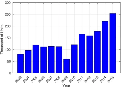
(38) 2. Introduction. years where the supply is expected to continue increasing.. Figure 1.1: Assembly line. 300. Thousand of Units. 250. 200. 150. 100. 50. 15. 14. 20. 13. 20. 12. 20. 11. 20. 10. 20. 09. 20. 08. 20. 07. 20. 06. 20. 05. 20. 04. 20. 20. 20. 03. 0. Year. Figure 1.2: Estimated worldwide annual supply of industrial robots While industrial robots are a fixture in the industry, advancements in safety systems, actuators and sensors are bringing robotics into new applications. Mobile robots promise to be the next frontier in service robotics. Although fixed robots will always have a place in the manufacturing industry, augmenting traditional robots with mobile robots adds flexibility to end-users in new applications..
(39) 1.1. Motivation. 3. 300. Thousand of Units. 250. Asia/Australia Europe America. 200 150 100 50. * 19 20. * 18 20. * 17 20. * 16 20. 15 20. 20. 14. 0. Year. Figure 1.3: Forecast supply of industrial robots. These applications include medical and surgical uses, personal assistance, security and rescue, warehouse, distribution, and even ocean and space exploration. Since 1998, about 220.000 service robots for professional use have been supplied. Due to the diversity lifespan of the products (underwater robots can have an average life time of 10 years in operation while defence robots may serve for short time), it is not possible to estimate how many robots are still in operation. The sales of service robots rose considerably in 2015, increasing 25 percent with respect to 2014 in professional use service robots, and 16 percent in domestic use ones. The most selling units are mobile platforms (domestic and professional use), and cleaning platforms (domestic use). Figure 1.4 shows how the supplies of service robots for professional use increase in every area in 2015 with respect to 2014. Figure 1.5 shows the forecast of service robots for domestic use and how the expected increment will be, from less than 10 million in the years 2014 and 2015 to more than 30 million in the period between years 2016 and 2019, only in household robots. With this forecast, it is clear that mobile robotics is a field of interest, as more robots will coexist with humans in uncontrolled.
(40) 4. Introduction 20. 2014 2015 Thousand of Units. 15. 10. 5. th er s lO Al. ru ct. io. n. ng an i C. on st. le C. tfo. M. ob. ile. Pl a. M. ed. rm. ic. s. al. el d Fi. en ef D. Lo. gi s. tic. ce. 0. Figure 1.4: Estimated worldwide annual supply of service robots 35. 2014 2015 2016-2019. 30. Thousand of Units. 25. 20. 15. 10. 5. 0 Household Robots. Entertainment & Leisure Robots. Figure 1.5: Forecast supply of service robots for domestic use environments. In order to achieve their tasks, mobile robotic platforms need to move in the environment, at the same time that assure their security and the environment one. To achieve an autonomous navigation, a mobile robot needs to perform several stages that are interconnected: perception, localisation, planning and control. Figure.
(41) 1.1. Motivation. 5. 1.6 shows these stages and the connection between them.. Map. Localisation. Planning. Perception. Control. Figure 1.6: Autonomous Navigation Stages Diagram An autonomous robot needs to perceive the environment, and it needs to know its own status, in order to perform the rest of stages. For this reason, it is equipped with two kind of sensors: proprioceptive and extereoceptive. Proprioceptive sensors, like odometers, gyroscopes or battery level sensors allow the robot to know its own state. Extereoceptive sensors, like Light Detection and Ranging (LIDAR), sonar, cameras or bumpers, allow the robot to perceive the environment. Usually an autonomous robot needs different and redundant sensors to achieve the autonomous navigation task with enough safety. For example, LIDAR and sonar are range measurement sensors. While LIDAR is a more precise sensor than sonar, its limitations are different, and, for example, it can not detect glasses. For this reason, an indoor autonomous robot usually needs to be equipped with both sensors. Sensor fusion techniques are generally used for working with dif-.
(42) 6. Introduction. ferent kind of sensors, improving the weakness of each one. Also, the information obtained from the sensors needs to be processed and interpreted in a way that the autonomous navigation systems can work with (for example, reducing the complexity of a depth image in a way that can be computed by the obstacle avoidance algorithm). Localisation stage answers the question “Where am I?”. The localisation can be performed with two different approaches, using a map or not. If the localisation is made without the use of maps, is commonly known as Dead Reckoning, and allows the system to know where the robot is at each time with respect to its origin. This localisation is made with one or more proprioceptive sensors like odometer, gyroscopes and accelerometers, or extereoceptive sensors like compass or Global Positioning System (GPS). Localisation using maps needs extereoceptive sensors to know where the robot with respect the map coordinates. Common techniques used in this localisation are Adaptive Monte Carlo Filter [Thrun et al., 2001] and Iterative Closest Point [Biswas and Veloso, 2012] which use range information obtained from the sensors and match this information with an a prior built map, aided with the dead reckoning navigation, in order to obtain the position of the robot inside the map. Maps can be built before the navigation, for example, using architectonic maps. But the environments, even the indoor ones, tend to slightly change with time. For this reason, maps can be more accurate if they are refined as the robot moves, adding information from the sensor measures. Also, there are techniques, known as Simultaneous Localization And Mapping (SLAM) [Newman et al., 2006] [Bekris et al., 2006], that build the map with the information from the sensors at the same time that localise the robot within the incrementally built map. Once a map is built and the robot is localised into it, to achieve an autonomous navigation the robot needs to execute the planning stage. This planning stage can be divided into global path planning and obstacle avoidance (or local navigation). Global path planning provides a series of way points that the robot must reach in order to achieve its final goal. This can be a slow task, depending on the.
(43) 1.1. Motivation. 7. complexity of the environment and the robot. While the robot is moving, unexpected obstacles can be detected by the sensors. Obstacle avoidance algorithms are in charge of reacting to these unexpected obstacles and avoiding them, assuring the integrity of the robot and the surroundings, at the same time that the robot tries to reach the way points obtained from the global path planning. Classic obstacle avoidance algorithms, like Vector Field Force (VFF) [Borenstein and Koren, 1989] and Potential Fields (PFs) [Hwang and Ahuja, 1992], work in a merely reactive way with the distance readings obtained by the sensors. These algorithms are light and fast but tend to produce not optimal motions and get stuck in local minima. Modern algorithms, like Beam Curvature Method (BCM) [Fernández et al., 2004], Nearness Diagram (ND) [Mı́nguez and Montano, 2004] obtain more information from the surroundings in order to plan the movement avoiding the obstacles, while obtaining smooth paths and avoiding the local minima problem. There are also algorithms that fuses the global navigation and obstacle avoidance stages ( [Montemerlo et al., 2009], [Kushleyev and Likhachev, 2009]) using the local information to replan the whole path in a faster way. Finally, Control stage is the one in charge of executing the commands obtained from the planning stage. This stage is related to the actuators of the robot and its complexity depends on the kind of driving of the autonomous platform. In the last years, autonomous navigation for robots and even vehicles has been improved with international competitions like DARPA Grand Challenge [Thrun et al., 2006] and DARPA Urban Challenge [Montemerlo et al., 2009], where car like robots were able to navigate autonomously reacting to unexpected obstacles. Figure 1.7(a) shows the winner of the 2003 edition and Figure 1.7(b) shows the winner of the 2005 edition. These robots are equipped with state of the art sensors and powerful computers and move in scenarios of known characteristics (for example, the traversable road is delimited with curbs). However, achieving autonomous navigation in previously unknown environments, and without this kind of expensive and redundant sensors, is still a challenge..
(44) 8. Introduction. Figure 1.7: DARPA Challenge Autonomous Robots. 1.2. Scope of this thesis. This thesis is placed within several projects: Abstraction, Synthesis and Integration of Information for Human-Robot Teams (ABSYNTHE)1 [Alonso et al., 2012], Plataforma Robótica Para La Investigación (PROPINA)2 and ROBOtic Guide for Shop (RoboShop)3 [Ocaña et al., 2014]. ABSYNTHE project main goals are the development of concepts, tools, and approaches for the collaborative production and application of high-level semantic descriptions of computational objects with a view to facilitate the joint intelligent processing and exploitation of knowledge by mixed and heterogeneous teams of human and robots. Some of the problems that the project needs to deal with are: • Qualitative Object Description: the collaboration between team members requires the ability to exchange information at various levels of abstraction. • Cooperative Robotics: the collaboration between humans and robots requires the capacity to map of perceptual information into symbols describing environmental features (topological maps). 1. Ministry of Economy and Competitiveness funded, code TIN2011-29824-C02-. 2. University of Alcalá funded, code UAH2011/EXP-013 University of Alcalá funded, code CCG2013/EXP-066. 02 3.
(45) 1.3. Proposal. 9. • Autonomous navigation in complex environments: it is needed that the robots in the team can navigate in realistic scenarios, with people moving around them and even changeable environments. • Integration of high-level sensor information: the perceptual information can be collected by distributed, multi-modal and different characteristics sensors used by the team members (humans and robots). So the developing of techniques that integrate and fuse this information are needed. This thesis is focused on the third point, the development of an autonomous navigation system that can react to moving and dynamic objects in the surroundings of the robot. With the experience of the real experiments made in the Robotics and eSafety Research Group (RobeSafe)4 with commercial robotics platform, PROPINA project proposes the design and development of our own robotic platform that can improve some of the flaws that the commercial platforms have. RoboShop project goal is to build a Robotic Guide for Shops. For this reason, PROPINA platform is used and equipped with more sensors (LIDAR, depth cameras, RGB cameras, Inertial Measurement Unit (IMU), etc.) to improve its usability. This Robotic Guide needs to cooperate with humans and needs to navigate autonomously in challenging environments.. 1.3. Proposal. Since 2004, the researchers of the RobeSafe research group at the Department of Electronics have been working in the autonomous navigation scope. Several important results were achieved in this scope. Some important works were, the development of a robot navigation system for indoor environments using signal strength from WiFi measurements and ultrasounds [Ocaña, 2005] [Ocaña et al., 2005], and the 4. www.robesafe.com.
(46) 10. Introduction. development of a robot navigation system based on Partially Observable Markov Decision Process (POMDP) using vision and proximity sensors [López, 2004] [López et al., 2005]. The RobeSafe research group has focused its efforts in some important aspects in order to develop these robot navigation systems. RobeSafe research group is interested in developing non-invasive systems, which means to use the own infrastructure of the environment without adding extra devices or technologies. Finally, developing solutions that work in real scenarios is always a premise for RobeSafe research group. The aim of this thesis is to develop a navigation system that can deal with dynamic obstacles and, even, changeable environments. This navigation system will not only assure the robot and environment safety, but also will produce smooth and fast trajectories. In order to do this, a perception system that can detect the variations in the robot’s surroundings is needed. The navigation system only uses the onboard sensors of the robot (especially LIDAR, IMU and odometry) in a way that beacons or devices in the environment are not needed.. 1.4. Document structure. After the introduction in Chapter 1, Chapter 2 contains a review of the most significant research in autonomous robot navigation, including obstacle avoidance and global path planning algorithms. In Chapter 3 a review of several commercial robotics middlewares is done. And, the proposal, development and simulation of our own robotic platform RoboShop. In Chapter 4, methods for autonomous navigation in dynamic environments are proposed. From local mapping stage, obstacle avoidance algorithms to global path planning ones. In Chapter 5 these algorithms are tested and evaluated, both in simulation and in real scenarios. Finally, Chapter 6 shows the conclusions and future work derived from this thesis dissertation..
(47) Chapter 2 State of the Art The main task of an autonomous mobile robot is to be capable of reaching several points in the environment, while assuring its own integrity and the environment safety. This task is known as navigation. Navigation can be divided into two different and complementary categories: global path planning and local navigation. Global path planning is the task that provides a series of positions or configurations that the robot must reach in order to reach a goal. To achieve this task the map needs to be known or, at least, partially known. As the robot moves, unexpected obstacles that have not been mapped before, or changes in the previously mapped environment, can happen and have to be measured by the available sensors (usually onboard the robot). These obstacles can block or affect the previously calculated path, so the robot must alter its route to the goal in order to avoid these unexpected obstacles, at the same time that the navigation has to be completed. This task is known as local navigation or obstacle avoidance. The line that separates local navigation and global path planning is sometimes very blurry. In order to clarify the main differences between them, these characteristics are pointed: • Local navigation: – It uses local information, usually obtained from onboard sensors.. 11.
(48) 12. State of the Art – It plans the next commands for the robot to execute (immediate or short time ahead). – It has near real time requirements. The algorithms are fast and work as reactive processes. – It allows the robot to travel safely. • Global path planning: – It uses known or partially known maps. – It plans for long distance and time periods. – It is a slower and deliberative process. – It allows the robot to avoid getting trapped in local minima scenarios, and fulfil its task.. However, in recent studies some of these classical characteristics are relaxed. For example, some local navigation algorithms use cumulative sensors data, or fuse with known maps, in order to plan the next optimal movement. Also, some global path planning algorithms can react to unexpected obstacles and replan the path in real time scenarios, fusing the local and global navigation in the same process. In the next sections a brief summary of several state of the art techniques that are used in local navigation and global path planning stages is performed. As the navigation task needs the perception and mapping stages, a brief summary of some helpful techniques is also included.. 2.1. Perception and Mapping. Before the navigation stage can be achieved, the robot needs to know the environment where it moves. For this reason the perception and mapping stages must be performed. In this section a brief summary of these stages is done. Perception is usually addressed with the onboard sensors of the robot, even when it can be complemented with intelligent environment sensors. Commonly used sensors in mobile robotics are: sonar.
(49) 2.1. Perception and Mapping. 13. sensors, LIDAR sensors, colour cameras, depth cameras, infrared sensors, etc. For local navigation purposes, the main information needed is if an area is traversable or not, or, what is the same, where are the obstacles surrounding the robot. For indoor mobile robots, it is assumed that any detection in the same height of the robot is an obstacle and the robot should not collide with it. For this reason the most used sensors are range only sensors (sonar, infrared, LIDAR), situated parallel to the floor. Nevertheless, for outdoor mobile robots and for some complex robots or environments, 3D information is needed. This information can be obtained from 3D-LIDAR, moving 2D-LIDAR, 2D-LIDAR positioned not parallel to the floor, stereo cameras, etc. In order to perform the local navigation or global path planning, a representation of the environment (map) is needed. Map can be local (it represents the surroundings of the robot, most suitable for local navigation) or global (it represents the whole environment where the robot moves). These maps can be built based on another map, based on measures from the sensors, based on expert knowledge, etc. Usually, indoor mobile robots move in planar environments that can be represented as 2D maps. These representations can be classified into topological and metric maps [Thrun, 1998]. Topological maps represent important zones and the relations between them. These maps tend to be simple, close to the human interpretation of the environment, they are very useful for top level tasks or path planning, but they are not suitable for local navigation. On the other hand, metric maps represent a continuous space discretised in a way that can be used by a robot. Figure 2.1 shows the same map represented in both ways: topological map represents each room and the transition between them and metric map divides the continuous map in cells of the same size. Building a metric map from continuous information needs a discretisation. One effective way to perform the discretisation in 2D environments are the cell decomposition methods. These methods divide the environment in cells that are connected with the adjacent ones and they allow to represent whether each cell is occupied (not traversable by the robot) or free (traversable by the robot). Even a.
(50) 14. State of the Art. Figure 2.1: Topological (left) and metric (right) mapping level of occupancy can be represented in a way that the loss of information caused by the discretisation, or the inaccuracies of the sensors measures can be directly used by the robot [Coué et al., 2006]. Some methods for cells discretisation are: • Approximate cell decomposition [Latombe, 1991a]: the environment is divided into cells of the same size and shape. It is an easy process but needs a trade-off between loss of information (the smaller the cell is, the lesser information will be lost) and size of the map generated (the smaller the cell is, the bigger the resulting map will be). • Adaptive cell decomposition: the environment is divided into cells of different size. One particular case of adaptive decomposition is the quadtree [Samet, 1988]. The method of dividing an environment into quadtrees begins with one cell that represents the whole map. If that cell is partially occupied, it is divided into four ones. That division is repeated on each cell until the resolution limit is reached or there are not partially occupied cells in the environment. This representation allows to have the same information as approximate cell decomposition using less memory. • Exact cell decomposition: the cells does not have a predefined size or shape and are determined based on the environment. The joins between cells represent the free space in the map. Figure 2.2 shows the three previously explained methods for cell.
(51) 2.2. Local Navigation. 15. discretisation applied to the same map where yellow colour represents free space, red colour represents obstacles and light red colour represents occupied cells after the discretisation.. (a) Continuous Map. (b) Approximate Cell Decomposition. (c) Adaptive Cell Decomposition. (d) Exact Cell Decomposition. Figure 2.2: Cells Discretisation Techniques. Credits to M. Huber The grid cell representation can be extended to full 3D maps, where the representation is usually based on VOLumetric piXELs (VOXELs) [Foley et al., 1994] instead of grid cells and it is useful for 3D navigation, as Unmanned Aerial Vehicles (UAVs) and Unmanned Underwater Vehicles (UUVs) need. Also, the grid map representation can contain more information apart from the occupancy value, allowing to fuse topological and metric maps by means of adding information, for example, about features on the environment that are situated inside each cell coordinate limits.. 2.2. Local Navigation. As a robot is moving, trying to reach a position or follow a path, unexpected obstacles, which have not been mapped before, could.
(52) 16. State of the Art. appear and be detected. Therefore, the robot needs to modify its path in order to assure the surroundings and its own integrity, at the same time that the assigned task is addressed. In this section a review of the state of the art techniques used for local navigation is performed. The simplest algorithms for local navigation are the bug based algorithms, such as Bug1, Bug2 (both algorithms in [Lumelsky and Stepanov, 1987]) and Tangent Bug [Kamon et al., 1996]. The behaviour of these algorithms is very simple: if an obstacle appears in the path of the robot, the robot follows the obstacle edge until it is avoided. These algorithms are very inefficient because the shortest or smoothest path to the goal is not calculated, and also potentially risky paths are performed because the robot do not react with enough anticipation to the obstacles. On the other hand, these algorithms can be used with very simple sensors such infrared or tactile ones. Figure 2.3 illustrates how the Bug2 algorithm works. The robot must follow the line that connects its initial position to the goal, but when an obstacle appears, it is surrounded until the robot crosses with the initial path and returns to it.. Figure 2.3: Bug2 Example. Credits to H. Choset Another approach for local navigation is the vector summation based algorithms. In this approach, each obstacle create a repulsive force around it at the same time that the goal creates an attractive force toward them. The addition of all these forces creates a safety.
(53) 2.2. Local Navigation. 17. path without obstacles which the robot can follow. Some implementations are VFF [Borenstein and Koren, 1989] and PFs [Hwang and Ahuja, 1992]. These algorithms are computationally simple and can work in controlled environments but they have several problems with some configurations of obstacles that can cause local minima and block the movement of the robot. In addition, they are suitable for omnidirectional robots, but, as they do not take into consideration the kinematics and dynamic restrictions, they do not work well in non-holonomic robots. Figure 2.4 shows the vector summation of the VFF algorithm, where the repulsive forces caused by the obstacles (Fr ), the attractive force of the goal (Ft ) and the resulting direction that the robot must follow R, are represented as vectors.. Figure 2.4: VFF Example. Credits to J. Borenstein et al. As indoor robots move in planar floors, the local navigation can be calculated in a cartesian space (x,y coordinates). There are techniques that use other searching spaces, like the histogram based methods, which divide the surroundings of the robot into angular sectors that can be transformed into a polar histogram. In this histogram, the proximity of an obstacle on each angular sector is represented, and it is easier to calculate the next orientation of the robot.
(54) 18. State of the Art. than in cartesian coordinates. Next orientation is obtained based on a cost function that have parameters such as security or distance to the goal. Algorithms of this kind are Vector Field Histogram (VFH) [Borenstein and Koren, 1991] and its extension Vector Field Histogram Plus (VFH+) [Ulrich and Borenstein, 1998]. These algorithms can deal better with uncertainties in the measurements and take into account kinematics restrictions of the robot. But they have some potential local minima problems, especially with “U” shaped obstacles. Figure 2.5 shows the transformation between the metric map (active window, shown below) to the polar histogram, where the height represents the proximity (and riskiness) of an obstacle, and the next action selection is performed.. Figure 2.5: VFH Example. Credits to J. Borenstein and Y. Koren Velocity Methods plan the next movement of the robot in the velocity space configuration instead of the cartesian one. In this way, velocity space maps the cartesian space (X-Y) into one that represents the linear and angular velocities of the robot, which made this.
(55) 2.2. Local Navigation. 19. very suitable for navigation in differential and holonomic robots, as a point in the velocity space corresponds to a velocity directly executable to the robot. In this transformation, the obstacles in the environment block some velocities and reducing the searching space. At each iteration, the algorithm selects the next reachable velocity to command to the robot using a cost function with parameters like security or smoothness. Some well known implementations of this algorithms are Dynamic Window Approach (DWA) [Fox et al., 1997] and Curvature Velocity Method (CVM) [Simmons, 1996]. Figure 2.6 shows the transformation between the cartesian space and the velocity space in DWA implementation, where the obstacles detected in the cartesian space (semicircle in left image) block possible velocities in the velocity space (dark areas in right image). These velocity methods are ones of the most used in mobile robotics but, as purely reactive methods, they have some local minima issues.. Figure 2.6: DWA Example. Credits to D. Fox et al. As the previous algorithms are merely reactive ones, they have potential local minima issues. In order to tackle this problem, another family of algorithms classifies the environment into different scenarios and uses different strategies of avoidance for each one. Implementations of these algorithms are ND [Mı́nguez and Montano, 2004] and Smooth Nearness Diagram (SND) [Durham and Bullo, 2008]. Figure 2.7 shows the scenarios classification for ND algorithm. The big issue of these algorithms is the complexity, due to several avoidance strategies have to be implemented, and the needing of good.
(56) 20. State of the Art. perception stage in order to classify the scenarios correctly.. Figure 2.7: ND scenarios classification. Credits to J. Minguez and L. Montano Another idea in order to avoid the local minima problem is to mix different techniques and create two different planners: one that selects a local goal within the surroundings of the robot and one that selects the next movement to reach this goal. Some of these methods are Lane Curvature Method (LCM) [Ko et al., 1998] and BCM [Fernández et al., 2004]. Both implementations obtain a local goal by means of dividing the surroundings of the robot (LCM into lanes, BCM into angular sectors) and they use CVM algorithm to reach this goal. Figure 2.8 shows the sectorisation of the free space (lighter areas) into lanes of the same direction using the LCM method. These methods are computationally more complex than the previous ones, as a two stage local navigation is performed. Instead of these deterministic or probabilistic approaches, there are a family of algorithms that uses soft-computing techniques to perform the local navigation. Some of these algorithms are based on Fuzzy Logic like [Faisal et al., 2013] [Dongshu et al., 2011] [Liang et al., 2011] [Lee et al., 2012] [Mbede et al., 2012] [Tang et al., 2013] or Neuro-Fuzzy Logic like [Mohanty and Parhi, 2012]. These algo-.
(57) 2.2. Local Navigation. 21. Figure 2.8: LCM Example. Credits to N. Y. Ko et al. rithms are easy to understand and to code but usually perform a merely reactive behaviour without achieving the best path to avoid the obstacles. It is assumed that the reviewed methods can achieve the local navigation, even in dynamic and changing environments where moving obstacles are. But this is only true under certain assumptions, especially that the robot can move faster than the obstacles. With this constrain, it is possible to avoid a moving obstacle in the same way than a static one. However, not dealing with the dynamic obstacles in a different way results in avoidance strategies that are not optimal and potentially risky, like moving toward approaching obstacles or crossing the robot and obstacle paths. To tackle this problem, there are algorithms that avoid the dynamic obstacles in a different way than the static ones. Apart from the perception of the velocity of the obstacles (which is not a matter of study in this dissertation), the first step is to calculate when a collision with a moving obstacle is possible. Work in Velocity Space is a method to deal with it. In [Fiorini and Shiller, 1993] the Collision Cone concept is proposed, a transformation between the cartesian positions where two mobile objects can collide into the velocity space. Based on this idea, a family of implementations known as Velocity-Objects algorithms appears. Figure 2.9 shows graphically.
(58) 22. State of the Art. the collision cone concept. The Collision Cone proposition only works with circular objects and it has been extended by [Chakravarthy and Ghose, 1998] to any irregular object. Some Velocity-Obstacle based methods are [Choi, 2014] where the collision cones are used to compute the path trajectory, [Masehian and Katebi, 2014] uses the collision cone to create angular sectors centred in the robot and choose the safer direction, [Alsaab and Bicker, 2014] where a simplified extension of the collision cones for irregular obstacles is used and [Zhong et al., 2011] where time constraints are introduced for rapidly planning. The big weakness of these methods is that the collision cone can only be calculated if the movement of the obstacles is linear.. Figure 2.9: Collision Cone Example. Credits to X. Zhong et al. There are also algorithms for local navigation that take dynamic obstacles into account without using the collision cone concept. [Yaghmaie et al., 2013] proposes an extension of the PFs algorithm, where the relative velocity of the obstacle affects the vector summation in order to avoid it. [Benzerrouk et al., 2012] uses the relative velocity of the obstacle to choose the direction of avoidance. The previous dynamic obstacle avoidance algorithms work with linear and instantaneous velocities of the obstacles. [Seder and Petrovic, 2007] proposes an extension of the DWA algorithm (Time Variant Dynamic Window (TVDW)) where the collisions are checked cell by cell in a grid map. It allows the avoidance of moving obstacles even.
(59) 2.2. Local Navigation. 23. if the movement is not linear, but increments the complexity of the searching (Figure 2.10 shows the cells intersections in the TVDW algorithm).. Figure 2.10: TVDW Example. Credits to M.Seder and I.Petrovic The main disadvantage of these methods, is that they guarantee an avoidance of the dynamic obstacles, but the safer and usually longer avoidance path is not achieved. In that way, the perception error in the velocities of the obstacles can affect these algorithms in a critical way, crossing the robot with the obstacle’s path. Therefore, if the obstacle increases its velocity or it is incorrectly perceived, it can crash with the robot. Lastly, there are algorithms that mix the local and global navigation. They use not only the next movement according to the current state of the robot, but also the future possible positions (in a local window). Some algorithms of this kind are Vector Field Histogram Star (VFH*) [Ulrich and Borenstein, 2000] and Dynamic Window Approach Star (DWA*) [Chou et al., 2011] where a tree of classic algorithms executions (VFH+ and DWA respectively) is built and the next movement is selected according to the whole path cost, and Vector Field Histogram with Time Dependent Tree (VFH*TDT) [Babinec et al., 2014] that modifies VFH* including the time in the planning to avoid moving obstacles. Table 2.1 shows a brief summary of the methods studied, and the pros and disadvantages of each family of algorithms..
(60) 24. Method. Pros Easy to implement. Simple sensors. Easy to implement. Suitable for omni-directional robots Easy to calculate next direction. Includes kinematic restrictions. Includes Kinematic restrictions. Suitable for differential and holonomic robots. Easy to implement. Human-like behaviour.. Bug Based Vector Summation Histogram Based Velocity Space Based Soft-Computing Based. Reduce local minima.. Two-Stage Planning. Reduce local minima problems.. Medium Time Planning. Most optimal path are calculated.. Velocity-Obstacles Based. Avoid dynamic obstacles.. Local minima issues Local minima issues Non optimal path. Complexity. Need good perception stage. Complexity. Slower methods. Complexity. Slower methods. Only linear velocities obstacles.. Table 2.1: Local Navigation Algorithms Summary. State of the Art. Environment Classification. Disadvantages Non optimal path. Potentially risky. Local minima issues Not Suitable for non holonomic robots..
(61) 2.3. Global Path Planning. 25. In this section a review of the local navigation techniques has been performed. However, it is important to remark that there is not a perfect algorithm that solves all the local navigation problems. The simpler algorithms can be used in smaller and computationally less powerful robots, even when the performance is worse than other more complex ones. It is also important to remark that in real scenarios is needed to avoid the dynamic obstacles taking into account their velocities and directions. In the literature some algorithms take this into account, but they deal with the immediate collision, and not the whole path that the obstacle is following.. 2.3. Global Path Planning. Given initial and goal states, the global path planning calculates a sequence of configurations that connects both states and avoids colliding with any obstacle. Global path planning can be used in a variety of robotic fields (including industrial arms, for example) but, in this section, some techniques that are used for path planning in mobile robots are surveyed. An Unmanned Ground Vehicle (UGV) can be considered as a solid rigid that moves in a 2D environment. So its configuration space is the cartesian coordinates (x and y) and its orientation. This configuration space can be increased if more variables are included like velocities, time, etc. The quality of a global planner can be measured with some parameters like: • Completeness: One algorithm is complete, if it is guaranteed that the solution is found. • Optimality: One algorithm is optimal, if it is guaranteed that the best solution (according to the evaluation function) is found. • Time/Space Complexity: the time and memory that the algorithm needs as the number of possible paths/states grows. In mobile robotics, time/space complexity is an important constraint, due to the systems real or near real time requirements. Also it is important that the completeness characteristic is achieved. The.
(62) 26. State of the Art. optimality of a global planner is a characteristic that can be relaxed: in real applications it is better to find a path that is not optimal (suboptimal) faster than a better path with time longer computation. If it is assumed that the robot moves in a 2D environment represented as a grid map, path planning can be performed. The best path that connects the two points can be evaluated using different metrics: less cells traversed, less turns performed, more distance to the obstacles, etc. One planning method for this grid maps is the Wavefront Based Algorithms. This family of algorithms calculates the value of each cell as the distance from the goal and propagates backward to the start point. Once the start position is reached, the planner can step back the cells with the less value in order to reach the goal. Some implementations are NF1 [Lengyel et al., 1990], NF2 [Latombe, 1991b] and Trulla [Murphy et al., 1999]. Figure 2.11 shows the path planned using a Wavefront algorithm in a grid map environment.. Figure 2.11: Wavefront Example Another planning method for grid based maps is the Global Potential Fields (GPFs) [Khatib, 1986]. Like the PFs algorithms for local navigation, each obstacle creates a potential field around it (greater values near the obstacle) and the goal creates another attractive potential field (lesser value near the goal). All the potentials are.
(63) 2.3. Global Path Planning. 27. added, and the path is reconstructed as a descending gradient from the start to the goal. This method is prone to local minima problem. Figure 2.12 shows the local minima issue: when all the potential fields are added, there is a point with a lesser value surrounding with bigger values in the way from the goal to the beginning.. Figure 2.12: Global Potential Field. Local Minima Problem Example One of the problems with the global path planning in grid maps is that the result is an unnatural path to follow, as it only considers 4 or 8 possibles changes of directions. There are techniques to smooth the path in order to be more natural to follow, but they need a two step algorithm and the computational cost is increased. On the other hand, the search space is reduced (x-y coordinates) and the path planning can be performed in a quick way. To cope with the unnatural path problem, and to reduce the search space at the same time, roadmap based representations appear. These methods find the connection between the free space as a set of lines or curves. Some methods based on the roadmap representation are: • Visibility Graphs [Nilsson, 1984]: connect each vertex of the obstacles in the environment with all the other vertex if the line does not cross any obstacle. Figure 2.13(a) shows an example of visibility graph and a path planned based on it..
(64) 28. State of the Art • Voronoi Diagrams [Choset and Burdick, 1996]: the roadmap consists of paths which are equidistant from all obstacles in the region. These paths merges in vertices forming a full roadmap where a planning stage can be executed. Figure 2.13(b) shows a Voronoi diagram with the path planned.. Figure 2.13: Visibility Graph and Voronoi Diagram Example • Probabilistic Roadmaps [Kavraki et al., 1996]: this technique tries to reduce the complexity of a continuous space into a discrete space, but instead of using characteristics of the environment, like Voronoi Diagrams or Visibility Graphs, it works creating nodes in the space and checking if these nodes can be connected. One commonly used variation of this technique is the Rapidly Exploring Random Trees (RRT) [LaValle and James J. Kuffner, 2001] which are more suitable for a rapid search and it captures the dynamic or even non-holonomic constraints. [Pepy et al., 2006] uses an RRT with kinematic constraints to plan a directly executable path for a mobile robot. • State Lattice [Pivtoraiko and Kelly, 2005]: this technique fuses the planning on configuration and cartesian states. The configuration space is discretised into configurations that are reachable from the previous one and they do not cross any obstacle. In that way, it is very useful to add dynamic and not holonomic constraints and to plan directly executable paths to a robot. Figure 2.14 shows a state lattice planner for a planetary rover..
(65) 2.3. Global Path Planning. 29. Figure 2.14: State Lattice Planning Example. Credits to M. Pivtoraiko and A. Kelly. The former methods (even the grid cell based ones) can be represented into a tree. This tree contains the possible configurations, the transition between them and the cost of performing this transition from a state to another. Figure 2.15 shows a typical decision tree, where each node can have an arbitrary number of successors, but each one only has one predecessor.. Figure 2.15: Decision Tree Example.
(66) 30. State of the Art. In order to search the best path into the tree, a graph search algorithm is needed. These algorithms are also used in a wide variety of applications like artificial intelligence, computer networking, etc. Some of these algorithms are the following ones: • Depth-first search: a branch is selected where the child is the better of its level and it is explored until the branch ends. If the goal is not reached, that particular branch is eliminated and the process is repeated. This search is simple and works well when there are multiple solutions to a problem, but does not guarantee that the best solution is found. • Breadth-first search: this search evaluates all the nodes at the same level in parallel. It guarantees that the optimal path is found and it works better than the Depth-First Search when there are a small number of solutions. Nevertheless the whole set of possible paths needs to be evaluated increasing the time required. • Iterative deepening [Korf, 1985]: this search is an iterative process of depth-first search with level limit. The optimal found tree can be found before the whole tree is explored, being faster than a breadth-first search, but it is slower than the depth-first search if there are many solutions. • Uniform-cost search: if there is a different cost to travel from one node to another in the graph, this solution can be used. It is similar to the breadth-first, but the nodes of same cost are evaluated instead of the nodes within the same level in the tree. One particular case of this search is the Dijkstra’s Algorithm [Dijkstra, 1959]. In that implementation (for global path planning) the cost of each node represents its distance to the goal. In real applications, creating and computing the whole graph could be not possible due to the size or complexity of the environment. In these cases, an heuristic search is used. These algorithms can not guarantee to find the optimal path to the goal but find, at.
(67) 2.3. Global Path Planning. 31. least, a suboptimal executable path. They use an evaluation function to score each node or state so a guided search can be performed. Some heuristic search algorithms for path planning are the following: • Best-first search [Winston, 1992]: it is depth-first algorithm where a heuristic is used, and indicates how far is each state from the goal. At each time, the best node in the frontier of evaluating nodes is selected and expanded. If the heuristic used is the distance from the node to the start the algorithm becomes an Uniform-Cost Search. If the metric is an estimate of the distance to the goal it becomes to a greedy search. Bestfirst search is faster than Dijkstra’s algorithm but ignores the cost of the whole path generated. • A* Search [Hart et al., 1968]: it is one of the most widely used search algorithm in robotics. It works in a similar way than the best-first search but the heuristic used is a combination of two metrics: the distance from the start and the estimated distance to the goal. The heuristic that estimates the cost of the node must be admissible. If the metric of the cost to the goal is stronger than the distance from the start, the algorithm works like a Dijkstra’s algorithm and it results in the optimal shortest path to the goal, but the search process is longer. If the weight distance from the start is the strongest, it works like a BestFirst Search, running faster but the optimal path may be not obtained. There are several variations of that heuristic that results in other algorithms, like Theta* [Daniel et al., 2014] and Block A* [Yap et al., 2011]. Even if these Heuristic searches are able to speed up the searching, when the environment is changing or partially unknown the replanning stage could not satisfy real time constraints. For this reason, algorithms for continuous or event driven replanning are used. One of the most used algorithm is the D* Algorithm [Stentz , 1994], an extension of the A* Algorithm. D* computes several paths at the start of the execution using an A* Algorithm and, if the map changes, is able to switch from one path to another and it repairs the previous one..
(68) 32. State of the Art. Several variants of A* and D* have been developed which are able to speed up the search, like Anytime A* [Hansen and Zhou, 2011], Anytime Repaired A* (ARA*) [Maxim Likhachev and Thrun, 2004], Focussed D* [Stentz, 1995], Framed Quadtree D* [Yahja et al., 1998], D*Lite [Koenig and Likhachev, 2002] and Constrained D* [Stentz, 2002]. The inclusion of dynamic obstacles into the global planning (or replanning) stage increments the search space. For example, if we consider the planning of a point-type agent in a grid type environment, it could be done in a 2D state space (x,y cartesian coordinates) but if we include the time, the complexity increments (3D state space, x,y cartesian coordinates and time). However, the previous techniques can be used but may not satisfy the time requirements of the real system. Nevertheless, works like [Kummerle et al., 2013] demonstrate that an autonomous robot navigation in real environments could be performed. During the Defense Advanced Research Projects Agency (DARPA) Urban Challenge, the Stanford Entry [Montemerlo et al., 2009] proposes the use of a state lattice for planning purposes mixing with an A* Search (Hybrid A*). As the time is implicit in the tree construction, planning in that kind of roadmap does not increases the complexity of the space from a cartesian one. Figure 2.16 shows the lattice planning of an autonomous car parking. [Kushleyev and Likhachev, 2009] and [Phillips and Likhachev, 2011] extend this lattice graph planning for indoor robots, where the transition space without moving in the space is needed. In this section a review of the global path planning for mobile robots has been performed. Some of these techniques, especially the ones based on Lattice States, have demonstrated that a navigation with dynamic environments can be performed. However, these techniques need heavy computation (at least, heavier than the local navigation techniques)..
(69) 2.4. Objectives. 33. Figure 2.16: Hybrid A* Example.. 2.4. Objectives. Once the state of the art has been summarized, and the flaws of the algorithms and improvement needed have been detected, the objectives of this thesis are the following: • Study of the several robotics middlewares available. This studio will be used to select one standard development platform where the algorithms can be applied in the maximum different robotics platforms and sensors as possible. • Study and comparison of local navigation algorithms. In this studio a real comparison of available local navigation algorithms will be performed, obtaining their pros and cons. Also, metrics for that comparison will be defined. • Study if the local navigation algorithms can be adapted for dynamic environments. • Obtaining the dynamics of the objects in the environment. Once the different objects are identified and classified, there is a need of modelling its movement and mapping that movement in a way that a local navigation algorithm can use it. • Integration of local navigation algorithms for dynamic obstacles in a full navigation framework, and test in real scenarios..
(70)
Figure


![Figure 2.2: Cells Discretisation Techniques. Credits to M. Huber The grid cell representation can be extended to full 3D maps, where the representation is usually based on VOLumetric piXELs (VOXELs) [Foley et al., 1994] instead of grid cells and it is usef](https://thumb-us.123doks.com/thumbv2/123dok_es/7293300.349414/51.748.168.622.229.527/discretisation-techniques-credits-representation-extended-representation-volumetric-instead.webp)
+7


Documento similar
The new approaches used in global path planning are Genetic Algorithm [4, 5], Neural Network [6] and Ant Colony Optimization (ACO) [7, 8]. Local path planning algorithms [9, 10]
Point cloud density analyses are presented in order to achieve the optimal rotation speed depending on the vehicle speed, distance to obstacles, etc.. The proposed system is able
Then, four measures based on color and motion are selected and examined in detail with different segmentation algorithms and standard test sequences for video object
To create genetic graph-based clustering algorithms and heuristics to improve the robustness and solutions of classical partitional clustering algorithms, and to study its
A new two-tier inverse technique for characterizing coaxial to waveguide transitions based on the use of genetic algorithms and the gradient descent method has been described and
A new two-tier inverse technique for characterizing jointly two coaxial to waveguide transitions and a device under test based on the use of genetic algorithms and
For this work we have implemented three algorithms: algorithm A, for the estimation of the global alignment with k differences, based on dynamic programming; algorithm B, for
From the available capacity of the underlying links as given by the linearized capacity region, we propose two routing algorithms (based on multipath and single path) that find
