Essays on the pharmaceutical industry

Chapter 3

The Effect of Generic Goods in the Pharmaceutical Industry

3.1

Introduction.

The so-called generic pharmaceuticals are those drugs for which their patents on the active

ingredient have expired. Their main characteristic is that they are sold at a cheaper price

than the already established, branded, medicine. In all but few cases, and referring to the

US, these generics are certified by the FDA (Food and Drug Administration) to be perfect

substitutes to the branded good in that their active ingredient is identical. Furthermore, they

are bioequivalent in the sense of being statistically indistinguishable from the established

product in key aspects of therapeutic use. However, they could vary in characteristics

such as shape, colour, packaging and labelling. Taking into account the fact that not all

consumers switch immediately to generics gives support to the idea of both goods not

being perfect substitutes.

During the 1980s, and especially in the US, there has been a dramatic increase in the spread

of generic drugs into markets for pharmaceutical products. For example, the volume of

sales of generics in the US accounts for 50% of the total volume of sales of prescribed

medicines. The mean in the European Union is around 35%. Both figures are very high

compared to the 2% in Spain (NERA 1997). However, Spain has been a peculiar country

in this respect, and we will not go into the details of why this has been so. The interested

reader will find a description of the Spanish pharmaceutical industry in N.E.R.A. (1997)

3.1 Introduction. 110

and Mestre-Ferrándiz (1999). These figures compared with the figures for 1984 (de Wolf

(1988)), as shown in Table 1, reflect the increase in the use of generics. The difference

between the US and Europe will be explained throughout the introduction.

Table 1 Total generic sales as % drug sales (1984,1996)

Year Year Country 1984 1996

❤❥✐❧❦✰♠♦♥

1.5 2

♣rq✰s

❦✰t✰✉✎✈①✇

q

✐✬②

3 35

③ ❤⑤④

15 50

Source: N.E.R.A. (1997) and de Wolf (1988).

The question that arises is why should we be interested in the production of generics and

why should they be economically viable? Due to their lower prices with respect to the

branded good, their production and use has been promoted by the public administration. In

the case of the US, for example, regulation of the pharmaceutical industry has seen different

phases. The Kefauver-Harris Act of 1962 enforced the FDA to issue more stringent rules

governing new drug testing and approval and reducing the effective patent protection period

by delaying the time of approval. This was due to the considerable monopoly power of

well-accepted drugs associated with informational failures, physician decision making and

third party payment, which reduced the price elasticity of demand to lower level than it

otherwise would be. At the same time, the ability of generics to compete was reduced

considerably because they had to duplicate the approval tests of the original drug, which

are generally very costly. The Waxman-Hatch Act (1984) tried to solve the two problems

of the reduced effective patent period and the high degree of difficulty for the generic drug

to enter the market once the patent had expired. This was done by extending the life of drug

patents and by simplifying the procedures required to approve generic substitutes without

3.1 Introduction. 111

tests to gain approval, but only required a bioequivalence demonstration to the pioneer’s

brand. This Act had the desired effect of stimulating competition against drugs whose

patent protection had expired.

In Europe, in many countries such as Belgium, France, Italy, Spain and the

Scandina-vian countries, the prescription pattern is influenced by making positive lists, or by placing

generics in a superior reimbursement category. Further, availability of generics is

encour-aged by abbreviated registration procedures in all European countries.

Economic motives other than promoting competition exist for encouraging the use and

production of generics both on the part of governments subsidising social health funds as

well as the part of consumers who pay for the medicines themselves. For instance, in Spain,

even though there is no specific policy to encourage the use of generics, the Ministry of

Health has announced the willingness to promote the use of generics in the National Health

System as a way of reducing costs. In other countries, such as France, whenever there exist

various medicines in the market with the same therapeutic value, general practitioners have

to prescribe the cheapest one. Furthermore, the French government has promised, through

the Agènce du Médicament, to double the number of generics before the end of 1999 (El

Pais, Thursday 19 February, 1998, p. 25).

One of the main factors that could explain generic substitution is the intensified pressure

from third party payers to minimise drug prices. In Caves et al. (1991) it is pointed out that

the substitution rates from branded to generic goods on Medicaid prescriptions more than

doubled prescriptions subject to reimbursement with respect to private insurers. Medicaid,

reimburse-3.1 Introduction. 112

ment limits to generic levels, if they exist. Furthermore, the growth of Health Maintenance

Organisations (HMOs) has also encouraged the use of generics. HMOs provide health

coverage to approximately 11% of the US population and on average, 31% of all HMO

pharmacy claims are for generics, compared to the 14% of insurance plans that cover

fee-for-service medical practice (Frank and Salkever 1997).

With respect to the supply side, it is argued in the literature that there seem to be little or

no barriers to entry. This implication is due to the provisions previously mentioned of the

Waxman-Hatch Act (Frank and Salkever 1992). Hence, the primary impediments seem

to come from the demand side. The first impediment refers to the accumulated goodwill

of branded producers, and any concerns about the difference in quality between the two

products. This point will be analysed later. The second impediment comes from the role

the pharmacist and the consumer play in deciding whether the original brand or the generic

is dispensed, once the physician has prescribed the drug and a generic is available. Before

1984, generic substitution was precluded once the physician had dispensed the brand name,

although these anti-substitution laws have now been universally rejected and pharmacists

are allowed to dispense generics. In Europe, however, generic substitution is not permitted

by the pharmacist. This is one of the reasons that could explain the pattern shown in Table

1.

The effect of the introduction of these generics on the price of the already-established

branded good has been a source of controversy. Various empirical estimates obtained to

measure the price response of branded goods in the face of entry give rise to different

3.1 Introduction. 113

during the early to mid-1980s, providing evidence that branded prices have increased

af-ter generic entry. Grabowski and Vernon (1992) obtain similar results when estimating the

effect of generic entry on prices for 18 high-sales-volume pharmaceutical products when

first exposed to generic competition during the mid 1980s. They compared prices before

generic entry and prices one year after entry, estimating a negative coefficient for the

num-ber of generics on the ratio of generic to branded price, which is of course consistent with

brand-name prices rising relative to generic prices after generic entry.

Caves et al. (1991) studied 30 drugs that lost their patent between the years 1976 and 1987.

They estimated a 2% reduction in brand name prices after patent loss, while entry by 20

generics caused a 17% price decrease in branded goods. These reductions were viewed as

very small price responses to entry.

However, it seems that the most widely accepted view is that brand-name prices have

in-creased after generic entry, rather than observing a two-way price rivalry between branded

and generic drug suppliers in order to deter entry. The most common scenario after generic

entry is then that the branded good’s price is maintained or increased, while losing market

share to lower-priced generics. Furthermore, as the number of generics increases, its price

is reduced.

This “Generic Competition Paradox”, as expressed by Scherer (1993), could be explained

by two institutional regularities. First, physicians tend to be reluctant to switch to generics.

Not only is the menu of drugs so vast that is virtually impossible for physicians to have

full information about all the possible alternatives available, but also the tendency to stick

3.1 Introduction. 114

branded goods in terms of general reputation makes physicians prescribe more expensive

drugs when cheaper ones exist. Pharmaceuticals are usually considered to benefit from

first-mover pricing advantages, as Grabowski and Vernon (1992) note:

“under conditions like those found in pharmaceuticals, first movers have natural prod-uct differentiation advantages that permit to charge high prices and retain substantial market shares.”

Hence, this strong brand loyalty has made physicians gain experience with the drug under

the period of patent exclusivity, making them insensitive to lower price opportunities. A

Dutch study (de Wolf 1988) interviewing 200 prescribing physicians shows their reluctance

to switch to generics since generic goods were badly represented in the doctor’s preferred

set of drug names. Secondly, and from the point of view of the consumer purchasing

drugs at the retail pharmacy, they usually lack the knowledge to evaluate the alternatives

to branded goods. This effect is reinforced with wholesalers and pharmacists who have

greater incentives to sell more expensive drugs, specially when pharmacies charge a fixed

percentage margin by product sold. This percentage, given a base retail price of 100, ranges

from 22.0 in the UK to 28.2 in Spain and 29.0 in France (NERA 1997). This is in contrast to

the USA, where Masson and Steiner (1985) provide evidence that generic products usually

carry higher gross margins to pharmacists which implies that both the consumer and the

pharmacist will be willing to substitute. This difference could be another reason which

could explain Table 1.

Hence, when the generic drug is introduced, we could say, without oversimplifying, that

drug buyers can be of two different types: those who are price-insensitive to generics and

intro-3.1 Introduction. 115

duced at a lower price, we have to take into account this market segmentation effect, since

we could argue that the branded-good seller prefers to increase price in the price-insensitive

market segment and desert the other segments rather than to reduce price to the price

sensi-tive customers. Hence, if we see from empirical results that branded goods have increased

in price, then we could reasonably argue that this price discrimination argument yield

supe-rior profits. This is the approach taken by Frank and Salkever (1992). They find conditions

supporting this empirical fact, and use for this purpose a market segmentation model with

one firm producing the branded good and a competitive fringe producing a homogeneous

generic drug i.e. they propose a model à la Stackelberg, with a leader - the pioneer

firm-and a follower - the competitive fringe.

Several authors have argued that first-mover advantages also exist in the market for

gener-ics. In particular, one hypothesis to explain large shares obtained by certain generic firms

is that if these introduce the generic several months before their rivals, they will obtain a

significant market advantage. Grabowski and Vernon (1992) indicate that for the sample

they study, for virtually all products the market leader is an early entrant. Of course, this

hypothesis is in line with branded good manufacturers producing their own generic

alter-native. Lobo (1996) argues that these firms have a natural advantage to produce their own

generic version. Furthermore, that can undertake the necessary studies and tests for the

cer-tification of the generic good during the patent life of their branded good, so that they are

the first in the market, earning higher market shares than their competitors as argued above.

en-3.1 Introduction. 116

try into the market to choose not to enter. The result could be a significant reduction in

competition due to the first-mover advantage of the brand-name manufacturer.

Therefore, if we take the US pharmaceutical sector as an example to be used where the

generic is well established, we could examine the situation when the generic is already in

the market. With this approach, we could have many possible situations, although we will

restrict ourselves to the pioneer firm producing its generic alternative, or rather, having a

third firm producing it. With this in mind, an interesting question then arises: are there

incentives for the pioneer firm to produce the generic itself ? This question could then be

extended to include consumer surplus, and hence say under what situation will consumer

surplus be greater.

In order to try to answer these questions, we will use a simple market segmentation model

with two firms producing a branded good with a different active ingredient. However, and

for simplicity, we will assume that both goods are perfect substitutes. As an example,

consider two branded drugs; Aspirin, whose active ingredient is acetylsalicylic acid, and

Gelocatil whose active ingredient is paracetamol. Some years ago, Bayer’s patent on

As-pirin expired and a generic is already in the market. The question that is posed in this paper

is then under what conditions will Bayer prefer to produce the generic itself, rather than

not producing it and letting a third firm produce it, always taking into account that whoever

introduces the generic, its price must be lower than the one for Aspirin. Of course, an

ob-vious question following the preob-vious one is under what situation consumers will be better

off. Note, that for simplicity, we assume that only the patent for Aspirin has expired and

3.1 Introduction. 117

The approach will be as follows. Due to the complexity of obtaining an analytical

re-sult with a very general model, we try to restrict ourselves in order for the analysis to be

tractable. Hence, we will give functional forms to the demand curves and cost functions,

and some “ad hoc” assumptions will be made in order to reduce the number of parameters.

The model will be set up in the following way: there exist two branded goods and a generic

of the one that has lost its patent. Due to the existence of the generic good, consumers

can be divided into two types, those whose demand for the branded good is unaffected by

the existence of the generic good (“loyal”consumers), and those whose demand is affected

by the generic good (“sensitive” consumers). Therefore, we have the consumers who may

buy the generic and whose demand could in principle depend positively on the price of the

branded good.

With respect to the technology of producing the branded and the generic good, we will

assume that the marginal cost of the generic drug is lower than the marginal cost of the

branded good. This is a realistic assumption since due to the characteristics of the two

goods, costs of packaging and labelling for the branded good are usually higher, since

generics usually come in white boxes without any labelling or colour. With respect to the

possibility of access to technology by the third firm, we will assume that technology is

freely available. However, if the pioneer firm decides to produce the generic, it does not

need to incur any extra fixed costs, since it has the technology required, which we assume

is similar to the one used to produce the branded good.

The paper is organised as follows. Section 2 introduces a general market segmentation

3.2 The Model. 118

solve the model under two alternative scenarios, (i) the firm producing the branded good

whose patent has expired also produces its generic alternative; (ii) a third firm produces the

generic good. In section 4 we compare the solutions obtained and define the conditions

un-der which the established firm will have incentives to produce the generic itself. Consumer

surplus is also compared in this section. Section 5 concludes and provides an agenda for

future research.

3.2

The Model.

3.2.1

General Set-up.

Consider a situation where to cure a certain illness (say “headache”) there exist two

alter-native drugs. For illustrative purposes, call them Aspirin, produced by Bayer, and denoted

as firm A, and Gelocatil produced by Gelos and denoted as firm B. However, for

simplic-ity, we will consider the case for these two goods to be perfect substitutes. Bayer has lost

its patent over acetylsalicylic acid several years ago and a generic substitute exists for

As-pirin, with the condition that its price has to be lower than the price of the branded good.

This generic can be produced only by one firm, either by the already established, pioneer,

firm or by a third firm which only produces the generic.

Market demand for branded medicines can be thought of as composed of two elements.

There are consumers insensitive to the generic, together with consumers whose decision

3.2 The Model. 119

Finally, demand for the generic drug depends on its own price as well as the price of the

branded alternatives.

To be precise, demand functions for branded goods are

❭ ✻ ❖ ✞ ✻ ❁✍✞ ❫ ❁✍✞ ✹♠❴ ✽ ❭ ✻ ✩✝❖ ✞ ✻ ❵ ✞ ❫✎❴ ✵ ❭ ✻✴ ❖ ✞ ✻ ❁✍✞ ❫ ❁✍✞ ✹♠❴ ❁ (77)

where☛❆✽ ✚ ❁❋❇

➥ ❢◆✐✽➠☛ ➥ ✞ ✹ ✽➟✞✭✠➂☛❿✌❅✄⑥✫✉å➐✆ ❲ ✄➭➹✯✄❘➘♥✄❘✠➂☛❿✌■❁ and ➀ ❭ ✻ ✩✝❖ ✞ ✻ ❵ ✞ ❫✝❴ ➀ ✞ ✻ ➼ ◗ ❁ ➀ ❭ ✻ ✩❘❖ ✞ ✻ ❵ ✞ ❫✎❴ ➀ ✞ ❫ ④ ◗ ❁ ➀ ❭ ✻✴ ❖ ✞ ✻ ❵ ✞ ❫✎❴ ➀ ✞ ✻ ➼ ◗ ❁ ➀ ❭ ✻✴ ❖ ✞ ✻ ❵ ✞ ❫✎❴ ➀ ✞ ❫ ④ ◗ ❁ ➀ ❭ ✻✴ ❖ ✞ ✻ ❵ ✞ ❫✎❴ ➀ ✞ ✹ ④ ◗ ❩

Demand for the generic drug is:

❭❘✹✾❖ ✞ ✻ ❁✍✞ ❫ ❁✫✞ ✹♠❴ ❁ (78) where ➀ ❭✝✹✾❖ ✞ ✻ ❁✍✞ ❫ ❁✍✞ ✹♥❴ ➀ ✞ ✹ ➼ ◗ ❁ ➀ ❭❘✹❸❖ ✞ ✻ ❁✍✞ ❫ ❁✍✞ ✹♠❴ ➀ ✞ ✻ ④ ◗ ❁ ➀ ❭❘✹✾❖ ✞ ✻ ❁✫✞ ❫ ❁✍✞ ✹♠❴ ➀ ✞ ❫ ④ ◗ ❩

As mentioned above, we present two alternative configurations of the supply side of the

market. In the first one, firm A produces both the branded good and its generic, while the

3.2 The Model. 120

3.2.2

Two firms (A, B) producing the branded goods; firm A produces

the generic.

The profit function for firm A is given by

①⑧⑦ ❖ ✞ ⑦ ❁✍✞ ✪ ❁✍✞ ✹♠❴ ✽P✞ ⑦ ⑧❭ ⑦ ✩✎❖ ✞ ⑦ ❁✍✞ ✪❤❴ ✵ ❭ ⑦ ✴ ❖ ✞ ⑦ ❁✍✞ ✪ ❁✫✞ ✹♠❴ ❙ ✵ ✞ ✹❑⑧➏❭✝✹➍❖ ✞ ⑦ ❁✍✞ ✪ ❁✫✞ ✹♠❴ ❙ (79) ✰ ✕ ⑦ ⑧❭ ⑦ ✩❅❖ ✞ ⑦ ❁✍✞ ✪②❴ ✵ ❭ ⑦ ✴ ❖ ✞ ⑦ ❁✍✞ ✪ ❁✍✞ ✹♥❴ ❁ ❭✝✹➍❖ ✞ ⑦ ❁✍✞ ✪ ❁✫✞ ✹♠❴ ❙ ❩

The profit function for firm B, which does not produce the generic, is given by

① ✪✾❖ ✞ ⑦ ❁✍✞ ✪ ❁✍✞ ✹♥❴ ✽✸✞ ✪ ⑧❭❘✪❛✩✝❖ ✞ ⑦ ❁✫✞ ✪❤❴ ✵ ❭✝✪ ✴ ❖ ✞ ⑦ ❁✍✞ ✪ ❁✍✞ ✹❛❴ ❙ (80) ✰ ✕ ✪❉⑧❭❘✪❛✩❘❖ ✞ ⑦ ❁✍✞ ✪❤❴ ✵ ❭❘✪ ✴ ❖ ✞ ⑦ ❁✍✞ ✪ ❁✍✞ ✹♠❴ ❙ ❩

We will consider the Nash (non-cooperative) equilibrium concept, where each firm chooses

the strategy that maximises its own profit, given the strategy of its rival. Formally, and

referring to our case, we have the following definition:

Definition 1 A vector of prices✞

❽ ✽ ❖ ✞ ❽ ⑦ ❁✍✞ ❽✪➙❁✍✞ ❽✹ ❴

is said to form a Nash equilibrium if and only if✞

❽ ⑦ ❁☞✞ ❽✹ ✽ ÷✜⑨❅⑩ ✞ ⑦ ❁✍✞ ✹ ö❉÷➂ø ①⑧⑦ ❖ ✞ ⑦ ❁✍✞ ✪ ❁✍✞ ✹♠❴ s.t. ✞ ✪ ✽❍✞ ❽✪

and✞ ❽✪ ✽ ÷✜⑨❅⑩ ✞ ✪ ö➄÷➂ø ① ✪❸❖ ✞ ⑦ ❁✍✞ ✪ ❁✫✞ ✹♠❴ ➶ ❩ ✆ ❩ ✞ ⑦ ✽P✞ ❽ ⑦ and✞ ✹ ✽➟✞ ❽✹ ❩

Notice that firm A’s strategy will be to choose (simultaneously) two prices✞

⑦

❁✍✞

✹

, subject

to the constraint that✞

✹ ➼❇❶ ✞ ⑦ ❁ with ◗ ❳ ❶ ❳▲✿ ❩

3.2 The Model. 121

to take into account the regulation procedures whereby the price of the generic good has to

be lower than the price of the branded good.

Hence, the problem for firm A becomes

❷✷✑❹❸ ù❻❺ ❵ ù û ①⑧⑦ ❖ ✞ ⑦ ❁✍✞ ✪ ❁✍✞ ✹♥❴ ➶ ❩ ✆ ❩ ✞ ✹ ➼✴❶ ✞ ⑦ ❩ (81)

Solving the problem amounts to formulate the following auxiliary Lagrangean function:

❼ ❖ ✞ ⑦ ❁✍✞ ✹ ❁✕❽ ❴ ✽✸✞ ⑦ ⑧❭ ⑦ ✩✝❖ ✞ ⑦ ❁✍✞ ✪❤❴ ✵ ❭ ⑦ ✴ ❖ ✞ ⑦ ❁✍✞ ✪ ❁✍✞ ✹♠❴ ❙ ✵ ✞ ✹●⑧⑨❭❘✹➙❖ ✞ ⑦ ❁✍✞ ✪ ❁✍✞ ✹♠❴ ❙ ✰ ✕ ⑦ ⑧❭ ⑦ ✩✝❖ ✞ ⑦ ❁✍✞ ✪❤❴ ✵ ❭ ⑦ ✴ ❖ ✞ ⑦ ❁✍✞ ✪ ❁✍✞ ✹♠❴ ❁ ❭✝✹➍❖ ✞ ⑦ ❁✍✞ ✪ ❁✍✞ ✹♠❴ ❙ (82) ✵ ❽ ❖ ❶ ✞ ⑦ ✰➲✞ ✹♠❴ ❁

whose Khun-Tucker conditions are

3.2 The Model. 122 ✞ ✹➑➵ ➀ ❼ ❖ ✞ ⑦ ❁✫✞ ✹ ❁❻❽ ❴ ➀ ✞ ✹ ➸ ✽ ◗ ❁ (86) ➀ ❼ ❖ ✞ ⑦ ❁✍✞ ✹ ❁❻❽ ❴ ➀ ❽ ✽ ❶ ✞ ⑦ ✰➲✞ ✹ ④ ◗ ❁ (87) ❽ ➵ ➀ ❼ ❖ ✞ ⑦ ❁✍✞ ✹ ❁❻❽ ❴ ➀ ❽ ➸ ✽ ◗ ❁ (88) ✞ ⑦ ④ ◗ ❁✍✞ ✹ ④ ◗ ❁❻❽ ④ ◗ ❩ (89)

Before going into the details, notice that from (3.83),

❭ ⑦ ✩ ✵ ❭ ⑦ ✴➙✵ ➵ ✞ ⑦ ✰ ➀ ✕ ⑦ ➀ ❭ ⑦ ➸▲➵ ➀ ❭ ⑦ ✩ ➀ ✞ ⑦ ✵ ➀ ❭ ⑦ ✴ ➀ ✞ ⑦ ✵ ➀ ❭ ⑦ ✴ ➀ ✞ ✹ ➀ ✞ ✹ ➀ ✞ ⑦ ➸ ✵ ➵ ✞ ✹ ✰ ➀ ✕ ⑦ ➀ ❭❘✹ ➸▲➵ ➀ ❭❘✹ ➀ ✞ ⑦ ✵ ➀ ❭❘✹ ➀ ✞ ✹ ➀ ✞ ✹ ➀ ✞ ⑦ ➸ ✵ ❽ ❶P➼ ◗

and given that❽ ❶ and ❭ ⑦ ✩ ✵ ❭ ⑦ ✴

are non-negative, as well as ❾

✞ ⑦ ✰✑❿ ★ ❺ ❿❻➀ ❺⑥➁ and ❾ ✞ ✹ ✰✭❿ ★ ❺ ❿❻➀ û ➁ ,

which are the mark-ups of price over marginal cost, then the response of

❭

⑦

and/or

❭❘✹

to

a change in✞

⑦

has to be negative for the first order condition to be satisfied. This price

response consists of a direct effect, which works through

❭

⑦

and

❭❘✹

, the latter being

non-negative while the former being non-positive, and an indirect effect, working through✞

✹

’s

reaction function in terms of✞

⑦

. From the assumption of the signs of the derivatives on

the demand functions, it implies that if ➀

✞ ✹ ➀ ✞ ⑦ ❯ ◗ ❁

the reduced form demand curve, which

3.2 The Model. 123

the ordinary demand curve, which takes into account both the direct and the indirect effect,

for the branded good for firm A.

From (3.85), we can say something similar with respect to the demand curve for the generic

good. When❽q✽

◗

❁

since

❭❘✹

✵

➵

✞

⑦

✰

➀

✕

⑦

➀

❭

⑦

➸▲➵

➀

❭

⑦

✩

➀

✞

⑦

➀

✞

⑦

➀

✞

✹

✵

➀

❭

⑦

✴

➀

✞

✹

✵

➀

❭

⑦

✴

➀

✞

⑦

➀

✞

⑦

➀

✞

✹

➸

✵

✵

➵

✞

✹

✰

➀

✕

⑦

➀

❭✝✹ ➸▲➵

➀

❭❘✹

➀

✞

✹

✵

➀

❭❘✹

➀

✞

⑦

➀

✞

⑦

➀

✞

✹

➸

➼

◗

❁

and given that

❭✝✹

❁

➵

✞

⑦

✰

➀

✕

⑦

➀

❭

⑦

➸

and

➵

✞

✹

✰

➀

✕

⑦

➀

❭❘✹

➸

are all non-negative, in addition to

the signs of the derivative of the demand functions, the effect of a change in the price of

the generic on the demand for the branded good of firm A and/or on the demand for the

generic must be negative for the first order condition to be satisfied. Again, we have two

effects, direct plus indirect, the indirect working through the price reaction function of✞

⑦

in terms of✞

✹

❩

Hence, if ➀

✞

⑦

➀

✞

✹

❯

◗

❁

then the reduced form demand for the generic will be

less own-price elastic than the ordinary demand curve.

Firm B, however, does not have to maximise profits subject to any constraint since it does

not produce the generic, and will have the following program:

❷✷✑❹❸

ù

þ

①

✪✾❖

✞

⑦

❁✍✞

✪

❁✍✞ ✹❛❴

❩

(90)

3.2 The Model. 124

➀

①

✪❸❖

✞

⑦

❁✍✞

✪

❁✍✞ ✹♠❴

➀

✞

✪

✽

❭✝✪❛✩

✵

❭❘✪ ✴➍✵

➵

✞

✪

✰

➀

✕

✪

➀

❭❘✪ ➸▲➵

➀

❭✝✪♥✩

➀

✞

✪

✵

➀

❭❘✪

✴

➀

✞

✪

➸

✽

◗

❩

(91)

The set of FOCs allows us to obtain a candidate equilibrium price vector✞

✩

❽

✽

❖

✞

✩

❽

⑦

❁✍✞

✩

❽

✪➔❁✫✞

✩

❽

✹

❴

up to satisfaction of the second order condition (SOC). Note that the 1 in the superscript

stands for scenario 1.

3.2.3

Two firms (A, B) producing the branded goods; firm C produces

the generic.

In this case, a third firm, C, produces the generic drug, again taking into account that the

price of the generic is lower than the price of the pioneer good. Now, we need to solve

the profit maximisation program for three firms, in order to obtain a Nash (noncooperative)

equilibrium, which can be defined formally in this scenario as:

Definition 2 A vector of prices✞

❽

✽

❖

✞

❽

⑦

❁✍✞ ❽✪➙❁✍✞ ❽✹

❴

is said to form a Nash equilibrium if, for every firm i=A,B,C, p✻

* maximises firm i’ s profit, given that the other firms play the strategy specified by✞

❽➂

✻

❩

The profit function for firm A will then be:

①⑧⑦

❖

✞

⑦

❁✍✞

✪

❁✍✞ ✹♠❴

✽P✞

⑦

⑧❭

⑦

✩✎❖

✞

⑦

❁✍✞ ✪❤❴

✵

❭

⑦

✴

❖

✞

⑦

❁✍✞

✪

❁✫✞ ✹♠❴

❙

(92)

✰

✕

⑦

⑧➏❭

⑦

✩✝❖

✞

⑦

❁✫✞ ✪❤❴

✵

❭

⑦

✴

❖

✞

⑦

❁✍✞

✪

❁✍✞ ✹♠❴

❙

❩

3.2 The Model. 125 ❷❈✑✔❸ ù❻❺ ①⑤⑦ ❖ ✞ ⑦ ❁✍✞ ✪ ❁✫✞ ✹♥❴ ❩ (93)

The first order condition that results is

➀ ①⑧⑦ ❖ ✞ ⑦ ❁✍✞ ✪ ❁✍✞ ✹♥❴ ➀ ✞ ⑦ ✽ ❭ ⑦ ✩ ✵ ❭ ⑦ ✴➙✵ ➵ ✞ ⑦ ✰ ➀ ✕ ⑦ ➀ ❭ ⑦ ➸▲➵ ➀ ❭ ⑦ ✩ ➀ ✞ ⑦ ✵ ➀ ❭ ⑦ ✴ ➀ ✞ ⑦ ➸ ✽ ◗ ❩ (94)

Note that firm B’s program will be symmetric to A’s and the FOC is the same as (3.91).

When firm C chooses✞

✹

in order to maximise its profit, he does so subject to the constraint

that✞ ✹ ➼✑❶ ✞ ⑦ ❩

Hence, we have to set up a Lagrangean for firm C, and solve using

Kuhn-Tucker conditions again. The program for firm C is then,

❷✷✑❹❸ ù û ① ★ ❖ ✞ ⑦ ❁✍✞ ✪ ❁✍✞ ✹♠❴ ✽➟✞ ✹❑⑧❭❘✹➍❖ ✞ ⑦ ❁✫✞ ✪ ❁✍✞ ✹♠❴ ❙✭✰ ✕ ★ ⑧❭❘✹✾❖ ✞ ⑦ ❁✍✞ ✪ ❁✍✞ ✹♠❴ ❙ (95) ➶ ❩ ✆ ❩ ✞ ✹ ➼✴❶ ✞ ⑦ ❁

resulting in the following Lagrangean function

❼ ❖ ✞ ✹ ❁✖➃ ❴ ✽✸✞ ✹❑⑧➏❭✝✹✾❖ ✞ ⑦ ❁✍✞ ✪ ❁✫✞ ✹♠❴ ❙✡✰ ✕ ★ ⑧➏❭✝✹➍❖ ✞ ⑦ ❁✍✞ ✪ ❁✍✞ ✹♥❴ ❙ ✵ ➃ ❖ ❶ ✞ ⑦ ✰➲✞ ✹♠❴ ❩ (96)

The Kuhn-Tucker conditions that come out from this maximisation program are

3.2 The Model. 126

✞

✹➑➵

➀

❼

❖

✞

✹

❁✖➃

❴

➀

✞

✹

➸

✽

◗

❁

(98)

➀

❼

❖

✞

✹

❁✖➃

❴

➀

➃

✽

❶

✞

⑦

✰➲✞

✹

④

◗

❁

(99)

➃

➵

➀

❼

❖

✞

✹

❁✖➃

❴

➀

➃

➸

✽

◗

❁

(100)

✞

✹

④

◗

❁✖➃

④

◗

❩

(101)

With this set of FOCs, we can find equilibrium prices✞

✴

❽

✽

❖

✞

✴

❽

⑦

❁✍✞

✴

❽

✪✙❁✫✞

✴

❽

✹

❴

up to satisfying

the SOCs. Note again that the 2 in the superscript refers to scenario 2.

3.2.4

Comparing the two scenarios.

Once we have solved for the equilibrium prices for the two different cases, and profits

are evaluated, we would like to compare the level of profits for firm A in order to see

under what conditions it has incentives to produce the generic itself. Another interesting

comparison would be to compute total consumer surplus for both situations, and compare

welfare levels. Recall that consumer surplus is the area under some individuals’s demand

curve. For example, for the individuals whose demand function is given by

❭

⑦

✩✎❖

✞

⑦

❁✍✞ ✪②❴

, we

get that the consumer surplus for those individuals between price✞

and an arbitrary price ➄

✞

3.3 A Specific Set-up. 127

✕✤✣

⑦

✩

✽ ➅

ù

➆

ù

❭

⑦

✩✎❖➈➇ ❁✍✞

✪❤❴

✔

➇

❩

(102)

Of course, we will be interested in comparing consumer surplus in equilibrium, so we

would like to evaluate them given equilibrium prices. Hence, and again using

❭

⑦

✩✎❖

✞

⑦

❁✍✞ ✪❤❴

as an example, we would like to find the consumer surplus for that segment at✞ ❽✪

i.e. we

are interested in

✕✤✣

⑦

✩

✽ ➅

ù

➆

ù➊➉

❭

⑦

✩✎❖➈➇ ❁✍✞ ❽✪

❴

✔

➇

❩

(103)

In order to find total consumer surplus, we need to sum up the consumer surplus for all the

demand curves for each scenario, so that we are able to compare them.

3.3

A Specific Set-up.

In order to obtain specific expressions for equilibrium prices and hence be able to compare

between the two scenarios proposed, we will give particular functional forms to the demand

and cost functions.

3.3.1

Two firms (A, B); firm A produces the generic.

The demand functions for the branded good for each firm will be, for firm A and firm B

3.3 A Specific Set-up. 128 ❭ ⑦ ✩❅❖ ✞ ⑦ ❵ ✞ ✪❤❴ ✽ ✑ ✩❣✩ ✰P✑ ✩ ✴ ✞ ⑦ ✵ ✑ ✩ ✝ ✞ ✪ ❁ (3.104) ❭ ⑦ ✴ ❖ ✞ ⑦ ❁✍✞ ✪ ❁✍✞ ✹♥❴ ✽ ✑ ✴ ✩ ✰P✑ ✴❣✴ ✞ ⑦ ✵ ✑ ✴ ✝ ✞ ✪ ✵ ✑ ✴ ✯ ✞ ✹ ❁ (3.105) ❭✝✪♥✩❘❖ ✞ ⑦ ❵ ✞ ✪②❴ ✽ ♦ ✩❣✩ ✰ ♦ ✩ ✴ ✞ ✪ ✵ ♦ ✩ ✝ ✞ ⑦ ❁ (3.106) ❭✝✪ ✴ ❖ ✞ ⑦ ❁✍✞ ✪ ❁✍✞ ✹♥❴ ✽ ♦ ✴ ✩ ✰ ♦ ✴❣✴ ✞ ✪ ✵ ♦ ✴ ✝ ✞ ⑦ ✵ ♦ ✴ ✯ ✞ ✹ ❩ (3.107)

The demand function that firm A will face for the generic is

❭❘✹✾❖ ✞ ⑦ ❁✍✞ ✪ ❁✍✞ ✹♠❴ ✽➠➹ ✩ ✰✲➹ ✴ ✞ ✹ ✵ ➹ ✝ ✞ ⑦ ✵ ➹ ✯ ✞ ✪ ❩ (108)

Notice that, by construction, all price coefficients have to be positive. With respect to the

cost function faced by firm A, it will be as follows:

✕ ⑦ ❖❪❭ ⑦ ✩ ✵ ❭ ⑦ ✴ ❵➏❭✝✹❤❴ ✽✓➋ ⑦ ✵ ✌ ⑦ ❖❪❭ ⑦ ✩ ✵ ❭ ⑦ ✴ ❴ ✵ ✌ ✹❛❭✝✹ ❁ (109)

where, by assumption, ✌

✹

➼

✌

⑦

❩

Notice that implicitly, with this cost function, we are

making the assumption that the costs for the branded and the generic good are independent.

However, we could have dependent costs, which could give rise to economies of scope.

Hence, the profit function for firm A becomes

3.3 A Specific Set-up. 129

Full derivations of the FOCs for firm A and B are available from the author. These are

used to find the equilibrium prices. However, and due to the large number of parameters

involved, the following assumptions are made.

Assumptions

❯

Due to the demand barriers to entry discussed in the introduction, we will assume

that the size of the market for branded goods is twice the size of the generic. Hence,

we have that ✑ ✩❣✩

✽✷✑

✴

✩

✽

♦

✩❣✩

✽

♦

✴

✩

✽❍✿

and therefore➹

✩

✽✱❃

❩

❯

There exists symmetry between the consumers buying either of the branded goods,

which implies having the same parameters on the demand functions faced by firm

A and B. The two branded goods are considered to be perfect substitutes, which

imposes further restrictions on the parameters. These assumptions imply that, for

the demand-insensitive segments, we have ✑

✩

✴

✽▲✑

✩

✝

✽

♦

✩

✴

✽

♦

✩

✝

✽▲✔

✩

❩

However,

we will assume that branded goods and the generic are not perfect substitutes,

but rather, there exists a degree of differentiation between them. Hence, in order

to take into account this, we require that ✑ ✴❣✴

✽➎✑ ✴ ✝

✽

♦

✴❣✴

✽

♦

✴ ✝ ✽❨➹

✴

✽Ý✔

✴

and

✑

✴ ✯

✽

♦

✴ ✯ ✽t➹

✝

✽➠➹

✯

✽❈✔ ✝ ❩

3.3 A Specific Set-up. 130

❭

⑦

✩✎❖

✞

⑦

❵

✞

✪❤❴

✽ ✿✈✰P✔ ✩❛❖

✞

⑦

✰➲✞ ✪②❴

❁

❭

⑦

✴

❖

✞

⑦

❁✍✞

✪

❁✍✞ ✹♠❴

✽ ✿✈✰P✔

✴

❖

✞

⑦

✰➲✞ ✪②❴

✵

✔

✝

✞

✹

❁

❭❘✪❛✩✝❖

✞

⑦

❵

✞

✪❤❴

✽ ✿✈✰P✔ ✩❛❖

✞

✪

✰➲✞

⑦

❴

❁

❭❘✪

✴

❖

✞

⑦

❁✍✞

✪

❁✍✞ ✹♠❴

✽ ✿✈✰P✔

✴

❖

✞

✪

✰➲✞

⑦

❴

✵

✔

✝

✞

✹

❁

❭✝✹➍❖

✞

⑦

❁✍✞

✪

❁✍✞ ✹♠❴

✽ ❃✢✰P✔

✴

✞

✹

✵

✔

✝

❖

✞

⑦

✵

✞

✪②❴

❩

❯

With respect to the technology, as stated before, the marginal cost of the generic

will be less than the marginal cost of the branded good. Firm A and B will have

identical costs with respect to the branded good each produces, so ✌

⑦

✽➎✌

✪

and

➋

⑦

✽✓➋

✪

✽✭➋

❩

For simplicity, we will set➋ ✽➛❃

. Again, for illustrative purposes,

we will assume that✌

⑦

✽➠✌

✪

✽❍✿❂❁

and✌

✹

✽

◗

❩

✿

❩

❯

The parameter ❶ measures how low the price of the generic should be compared to

the price of the pioneer good. We will consider as an example the case for Spain,

where the price of the generic has to be, at least, 20% less than the original brand.

Hence, we fix ❶

✽

◗

❩

✿

for illustrative purposes.

Once we have imposed these assumptions, the Kuhn-Tucker conditions for firm A and first

order conditions for firm B respectively are shown in Appendix 1.

Consider first the case❽ ✽

◗

❁

which implies that the constraint is non-binding. Equilibrium

prices then depend on ✔

✩

❁❋✔

✴

❁

and ✔ ✝ ❩

Under this situation, for prices and quantities to be

3.3 A Specific Set-up. 131

Hence, let us consider ❽Ý❯

◗

❁

which implies ✞

✹ ✽ ◗ ❩ ✿ ✞ ⑦

i.e. the constraint is totally

satiated. When solving for the equilibrium prices, we obtain the following:

✞ ✩ ❽ ⑦ ✽ ❃✉ê ◗✭❖ ✔ ✩ ✵ ✔ ✴ ❴ ✵ ❾ ◗ ✔ ✝ ✰ ✂ ◗ ✔ ✝ ❖ ✔ ✩ ✵ ✔ ✴ ❴ ✵ ✿ ✿ ❃✉✔ ✴ ✔ ✩ ✵ ✿ ◗ é☞✔ ✴ ✴ ✵ é❂ý✉✔ ✴ ✩ ❃✶✿ ❾ ✔ ✴ ✔ ✩ ✰P❃ ◗❂◗ ✔ ✝ ❖ ✔ ✴✏✵ ✔ ✩❡❴ ✰t✿ ✂ ✔ ✴ ✝ ✵ ✿➺ê✉è❂✔ ✴ ✴ ✵ é❂ý✉✔ ✴ ✩ ❁ ✞ ✩ ❽ ✪ ✽ ê✓é❂ý✉✔ ✴ ✩ ✵ è✓ý ◗ ✔ ✩ ✵ è❂è ◗ ✔ ✴ ✔ ✩ ✰Pý ◗❂◗ ✔ ✝ ✔ ✩ ✰t✿ ✂ ◗ ✔ ✴ ✝ ✵ ✿➺❃❂é ◗ ✔ ✴❆✵✮✂ ✿➺ý✉✔ ✴ ✴ ✰ ❾❂❾ ◗ ✔ ✝ ✰ ❾ ê ✂ ✔ ✝ ✔ ✴ ý ❖ ❃✯✿ ❾ ✔ ✴ ✔ ✩ ✰➟❃ ◗❂◗ ✔ ✝ ❖ ✔ ✴✏✵ ✔ ✩❡❴ ✰❥✿ ✂ ✔ ✴ ✝ ✵ ✿➺ê❂è✉✔ ✴ ✴ ✵ é❂ý✉✔ ✴ ✩ ❴ ❁ ✞ ✩ ❽ ✹ ✽ ❾ ❖ ❃✉ê ◗✇❖ ✔ ✩ ✵ ✔ ✴ ❴ ✵ ❾ ◗ ✔ ✝ ✰ ✂ ◗ ✔ ✝ ❖ ✔ ✴❆✵ ✔ ✩❡❴ ✵ ✿ ✿ ❃✉✔ ✴ ✔ ✩ ✵ ✿ ◗ é☞✔ ✴ ✴ ✵ é❂ý✉✔ ✴ ✩ ❴ ý ❖ ❃✯✿ ❾ ✔ ✴ ✔ ✩ ✰➟❃ ◗❂◗ ✔ ✝ ❖ ✔ ✴❆✵ ✔ ✩❡❴ ✰t✿ ✂ ✔ ✴ ✝ ✵ ✿➺ê❂è✉✔ ✴ ✴ ✵ é❂ý✉✔ ✴ ✩ ❴ ❩

These prices need to satisfy the non-negativity constraint. If this is so, the equilibrium

prices depend on the three parameters that we are interested in, and we can now evaluate

the equilibrium profits of both firms, to obtain①

✩ ❽ ⑦ ❖ ✞ ✩ ❽ ⑦ ❁✍✞ ✩ ❽ ✪✙❁✍✞ ✩ ❽ ✹ ❴ and① ✩ ❽ ✪ ❖ ✞ ✩ ❽ ⑦ ❁✍✞ ✩ ❽ ✪➔❁✫✞ ✩ ❽ ✹ ❴ which

will depend on the same three parameters. Recall that the 1 refers to scenario 1.

3.3.2

Two firms (A, B) producing the branded goods; firm C produces

the generic.

Under this scenario, we need to introduce a third firm which produces the generic. The

maximisation programs for firms A and B are given by (3.93) and (3.90) respectively.

Notice, that due to the assumptions, and since firm A does not produce the generic anymore,

both firm A and B are identical, so in equilibrium they will have same prices and hence

same profits. With this in mind, we obtain the FOCs for the three firms, which are shown

in Appendix 2.

We solve first when❽q✽

◗

❩

Again, prices and/or quantities are positive only if some

3.4 Comparison of Both Scenarios. 132

When❽◆❯

◗

❁

the constraint will be satiated, and we obtain the following equilibrium prices

✞

✴

❽

⑦

✽ ý

➵

❃

✵

✔

✩

✵

✔

✴

ý✉✔

✩

✵

ý✉✔

✴

✰

❾

✔

✝

➸

❁

(3.111)

✞

✴

❽

✪ ✽ ý

➵

❃

✵

✔

✩

✵

✔

✴

ý✉✔

✩

✵

ý✉✔

✴

✰

❾

✔

✝

➸

❁

(3.112)

✞

✴

❽

✹

✽

❾

➵

❃

✵

✔

✩

✵

✔

✴

ý✉✔

✩

✵

ý✉✔

✴

✰

❾

✔

✝

➸

❩

(3.113)

Due to our assumptions, we obtain that in equilibrium, ✞

⑦

and ✞

✪

will be equal.

No-tice that since the constraint is satisfied with equality, the firm producing the generic will

only have to set its price equal to

◗

❩

✿ ✞

⑦

❩

With these prices, we can then evaluate the

equi-librium quantities to obtain the equiequi-librium profits①

✴

❽

⑦

❖

✞

✴

❽

⑦

❁✍✞

✴

❽

✪✙❁✍✞

✴

❽

✹

❴

, ①

✴

❽

✪

❖

✞

✴

❽

⑦

❁✍✞

✴

❽

✪➔❁✍✞

✴

❽

✹

❴

and

①

✴

❽

★

❖

✞

✴

❽

⑦

❁✍✞

✴

❽

✪✙❁✍✞

✴

❽

✹

❴

in terms of the three parameters we are interested in. Note that for both

cases, the equilibrium prices we have found satisfy the second order conditions.

3.4

Comparison of Both Scenarios.

3.4.1

Profits.

In order to compare profits, we have to do some kind of simulation due to the fact that

the conditions that arise when comparing profits with three parameters are very difficult to

analyse analytically. Hence, the strategy followed will be to fix some parameters, and do

some comparative statics with the others, and see whether the conditions that give rise to

higher profits in one scenario or the other are consistent as we change the parameters.

The first exercise is to fix ➌➎➍ , increase ➌✔➏➑➐ and find under what conditions for ➌✔➒❍➐ firm A

3.4 Comparison of Both Scenarios. 133

intervals for➌✦➒ that ensure that prices, quantities and the Lagrange multipliers in

equilib-rium are all non-negative. As an illustrative example, we will present the results obtained

with ➌➎➍❉➓❊➔➎→✠➣↔➐ and ➌✦➏ increasing. Note that the exercise was repeated for different fixed

values of ➌➎➍ and the results did not change qualitatively. Moreover, increasing ➌➎➍ and ➌✔➏

at the same time has the same qualitative results as keeping ➌➎➍ fixed. A summary of the

results are shown in Table 2. Notice that there exist more solutions, but we only consider

non-negative values for➌✔➒➑→

Table 2 Range for d3 for which prices and quantities for case 1 and 2 are non-negative.

➌➎➍❨➓✓➔➎→✠➣ ↕✎➙✔➛❬➜↔➝➟➞❥➠✌➡➢➌✦➒✬➤✌➙❹➥❝➦➧➤✻➞✞➨↔➦♦➛❬➜ ↕✎➙✔➛❬➜↔➝➟➞❥➠✌➡➩➌✔➒➫➤➑➙❹➥❝➦➭➤✌➞❬➨➯➦➲➛✞➜ ➌✔➏ ➳

➍➭➵➏❝➸

➺

➐➲➳ ➍➭➵➏❝➸

➻

➐➲➳ ➍➭➵➏❝➸ ➼ ➽

➔ ➾ ➍➭➵➏❝➸

➺

➍

➐❅➾ ➍➭➵➏❝➸

➺

➏

➐❅➾ ➍➭➵➏❝➸

➻

➍

➐❅➾ ➍➭➵➏❝➸

➻

➏

➐❅➾ ➍➭➵➏❝➸ ➼ ➽

➔

➔↔→➚➣ ➔➶➪✗➌✔➒➟➹✙➔➎→✠➣↔➘ ➔➴➪✴➌✔➒➢➹✙➔➎→✄➷❹➬ ➘ ➔➶➪✗➌✔➒➟➹✙➔➎→✄➮✜➱ ➔➴➪✴➌✔➒➢➹✙➔➎→✄➬❹➮ ➘✜→➚➣ ➔➶➪✗➌✔➒➟➹✭➘❹→✣➘✌✃ ➔➎→✄➔✜➱➶➪✗➌✦➒➟➹✙➔↔→✠❐❹❐

❒

➔➶➪✗➌✔➒➟➹✭➘❹→✠➣↔➘ ➔➎→ ❒❹❒

➪✗➌✦➒➟➹✙➔↔→➚➣↔➘

❒

→➚➣ ➔➶➪✗➌✔➒➟➹✭➘❹→✄➮❹➷ ➔➎→❮➱✦✃✛➪✗➌✦➒➟➹✭➘✜→✠➮❹➷

Taking into account that➌✔➒ has to lie in the regions shown in Table 2 for the specific values

of ➌➎➍ and ➌✔➏❍➐ we can compare profits for firm A under both scenarios, for this illustrative

example, and see whether it will have incentives to produce the generic itself.

Comput-ing profits for firm A (note that we also include the cases for all other profit levels to be

positive), we get the results which are summarised in Table 3.

Table 3a Range for d3 for which profits for case 1 and 2 are non-negative.

➌➎➍❨➓✓➔➎→✠➣ ↕✎➙✦➛✞➜↔➝➟➞❥➠✻➡➢➌✔➒➫➤➑➙❹➥❝➦➭➤✌➞❬➨➯➦➲➛✞➜ ➌✦➏ ❰

➍➭➵➏❝➸ ➺ Ï

➳

➍➭➵➏❝➸

➺

➐➲➳ ➍➭➵➏❝➸

➻

➐➲➳ ➍➭➵➏❝➸ ➼ Ð

➐❅❰ ➍➭➵➏❝➸ ➻ Ï

➳

➍➭➵➏❝➸

➺

➐♦➳ ➍➭➵➏❝➸

➻

➐➲➳ ➍➭➵➏❝➸ ➼ Ð

➐❅❰ ➍➭➵➏❝➸ Ñ Ï

➳

➍➭➵➏❝➸

➺

➐➲➳ ➍➭➵➏❝➸

➻

➐➲➳ ➍➭➵➏❝➸ ➼ Ðr➽

➔

➔➎→✠➣ ➔➶➪✴➌✔➒➩➹✥➔➎→➚➣➯➘

➘ ➔➎→✠➷

❒

➪✴➌✔➒➢➹✙➔➎→✄➮✜➱ ➘❹→✠➣ ➔➎→➚➣✜✃➴➪✴➌✔➒➢➹✭➘❹→✣➘✌✃

❒

➔➎→✠➮

❒

➪✴➌✔➒➢➹

❒

→

❒

➱

3.4 Comparison of Both Scenarios. 134

Table 3b Range for d3 for which profits for firm A are greater in case 1.

➌➎➍➫➓✓➔↔→➚➣ ↕✎➙✦➛✞➜↔➝➟➞❥➠✻➡➢➌✔➒➫➤➑➙❹➥❝➦➭➤✌➞❬➨➯➦➲➛✞➜ ➌✔➏ ❰

➍♦➸ ➺ Ï

➳

➍➭➵➏❝➸

➺

➐➲➳ ➍➭➵➏❝➸

➻

➐➲➳ ➍➭➵➏❝➸ ➼ ÐÒ➽

❰

➏❝➸ ➺ Ï

➳

➍➭➵➏❝➸

➺

➐➲➳ ➍➭➵➏❝➸

➻

➐➲➳ ➍➭➵➏❝➸ ➼ Ð ➔➎→➚➣ ➔➶➪✴➌✔➒➩➹✥➔➎→✠➬✜➬

➘ ➔➎→✠➔❹✃➴➪✴➌✔➒➢➹✭➘❹→✄➔❹➬ ➘❹→➚➣ ➔➎→❁➘➑✃➴➪✴➌✔➒➢➹✭➘❹→❮➱✔➬

❒

➔➎→✠➷❹➣➴➪✴➌✔➒➢➹✭➘❹→✄➮❹➬

❒

→➚➣ ➔➎→➚➣✁➷➶➪✴➌✔➒➢➹

❒

→

❒

➬

Therefore, combining Tables 2 and 3 together, it seems that firm A will always have

incen-tives to produce the generic itself. Note that we are not interested in the numbers per se,

but in the conditions that give rise to firm A making higher profits when it produces the

generic.

Furthermore, under the range for ➌✔➒ that satisfies the required conditions, we get that the

price that firm A is able to charge the consumers for its branded good can be higher for the

first case i.e. when it produces the generic. Therefore, firm A is able to increase the price

of its branded good under scenario 1 and make higher profits. Moreover, by producing the

generic itself, firm A can charge a higher price for the generic than otherwise would charge

firm C in scenario 2. Of course, this is so since the regulatory constraint is always satisfied,

so that once firm A produces the generic, its price rises proportionately with the increase in

the price of the branded good of firm A. Hence, the production of the generic good enables

firm A to charge a different price than its competitor, something which is not profitable

when there are three firms in the market.

An intuition behind this result could be that firm A is able to discriminate when it introduces

3.4 Comparison of Both Scenarios. 135

good producers are the same. Furthermore, in order for firm A to be profitable producing

the generic, it requires a price insensitive market segment.

For firm B, the results obtained show that it can charge higher prices under scenario 1, and

it will be better off by doing so. However, we can say that firm B will earn lower profits

than firm A in case 1, for the interval of parameters satisfying the restrictions, although the

same level for case 2. Firm C will only make positive profits when➌Ó➍ takes low values.

3.4.2

Consumer Surplus.

Following a similar procedure as when comparing profits, and due to the problem of

ob-taining analytical results which were impossible to analyse, some simulation results are

presented. The idea is the same as before; we fix some parameter and we let the others

change, while satisfying the restrictions imposed at the beginning. Again, we fix ➌➎➍ for

convenience, and we change ➌✔➏ , while calculating the range for the possible values of ➌✔➒

that satisfy the assumptions. Note that, as in the previous section, we also let ➌➎➍ change,

and the qualitative results did not change.

In order to calculate consumer surplus, the approach taken is as follows: since we are

interested in calculating it in equilibrium, we find the area under each demand curve (➾

➺

➍

to ➾

➼

) from its own equilibrium price up to the intercept, taking the other prices as fixed

and equal to their equilibrium values. Then, we add them up for both scenarios.

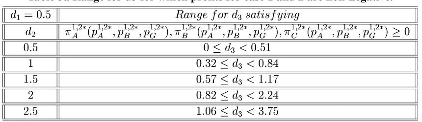
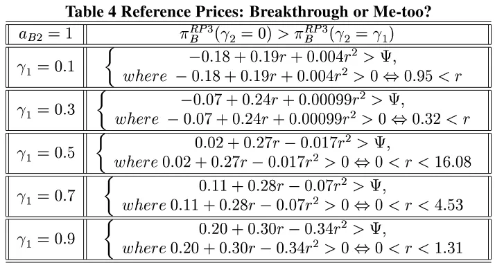
As we did before with profits, we can take ➌➎➍➴➓Ô➔➎→✠➣ as an illustrative example. Table 4

3.5 Conclusions and Future Research. 136

the consistent range of ➌✔➒ , consumer surplus is greater when there are three firms in the

market i.e. Õ✵Ö

➏

➽

Õ✵Ö

➍

.

Table 4 Range for➌✦➒ for which consumer surplus for case 2 is greater

➌➎➍➫➓✗➔➎→✠➣ ↕✎➙✦➛✞➜↔➝➟➞❥➠✻➡➢➌✔➒➫➤➑➙❹➥❝➦➭➤✌➞❬➨➯➦➲➛✞➜

➌✔➏ Õ✵Ö

➏

➽

Õ✵Ö

➍

➔➎→✠➣ ➔➶➪✴➌✔➒➩➹✥➔➎→➚✃✜➣ ➘ ➔➶➪✴➌✔➒➩➹❂➘❹→✠➔✜➷ ➘❹→✠➣ ➔➶➪✴➌✔➒➩➹❂➘❹→✄➱➎➘

❒

➔➶➪✴➌✔➒➩➹❂➘❹→➚✃✁❐

❒

→✠➣ ➔➴➪✗➌✦➒➟➹

❒

→❁➘✌✃✁➬

3.5

Conclusions and Future Research.

Using a market segmentation model we have illustrated that, under our assumptions, firm

A will have an incentive to produce its generic alternative, rather than having a third firm

producing it, once the patent for its active ingredient has expired. The model assumes

that there exist two firms, producing two drugs with a different active ingredient, although

we treat them as perfect substitutes. However, we do allow for a degree of differentiation

between the branded and the generic good. This is done to take into account empirical

results that suggest that consumers do not switch immediately to generic drugs once they

are introduced. We assume that the marginal cost of the generic is less than the marginal

cost for the branded good. This could be regarded as a realistic assumption if we take into

account the characteristics of both goods, since the latter usually comes in a box with more

labelling, while the former comes in a white box.

We assume symmetry in the demand functions for the branded goods that firm A and firm

3.5 Conclusions and Future Research. 137

the basis of different responses of consumer’s demand of branded goods: some consumers’

demands are not dependent on the price of the generic (intuitively, and loosely-speaking,

they could be treated as “loyal” customers), while some are affected by it.

In order to make the analysis tractable, we do some simulation exercise to see whether the

firm whose patent for its active ingredient has expired has incentives to produce the generic

alternative. For illustrative purposes, we give a full set of results for particular values of

the parameters. The qualitative conclusions reached are similar with many other set of

values. We find, that given our assumptions, this firm will always have the incentive to

produce it. The firm uses the generic as a means to increase the price of its branded good

in order to obtain higher profits. Furthermore, this firm can charge a higher price for the

generic good compared to the price that would otherwise be set by a third firm producing

the generic alternative. This is due to the fact that the regulatory constraint, that the price

of the generic has to be less than or equal than the price of the pioneer good, is satisfied

with equality. This implies that whoever produces the generic has incentives to introduce it

with the highest price possible. Hence, since firm A uses the production of the generic as a

means to increase the price of its branded good, the price of the generic rises accordingly.

Notice that due to the assumptions of firm A and firm B being identical with respect to both

the demand functions they face and the costs of producing the branded good, they obtain

the same profits when a third firm produces the generic. Hence, when firm A produces the

generic, not only is it better off with respect to the case when there are three single product

3.5 Conclusions and Future Research. 138

Consumer surplus is lower under the first scenario, where there are only two firms in the

market. This is because of the strategy by firm A of producing the generic, in order to

increase the price of both goods.

The policy implications of these results are that, since the promotion of generic drugs is

coming from many different sides of the economy, from a social point of view, their entry

should be encouraged through firms not producing their own branded good, but rather

through firms who specialise in the production of generics. Hence, entry barriers to these

firms should be made as low as possible. However, if we see in reality that existing firms

producing branded goods decide to produce generics themselves, it could be a signal that

they are using these as a means of increasing the price of the branded goods in order to

increase their profits. This is the pattern that we are observing now, since nowadays we

are confronted with many “branded generics” and higher prices for the branded goods.

These firms not only use their natural advantage of producing their generic alternative in

order to gain the first mover advantages in the market for generic goods, but also use them

strategically to increase the price of the branded good to exploit their loyal customers.

Hence, this paper is in line with those that estimate an increase in the price of the branded

good once the generic drug is in the market. However, this increase in price results from

the strategic use of their generic alternatives by already established firms.

Of course, possible extensions to the model are plausible. For example, when we

con-sider firm A introducing the generic, we assumed that costs are independent. However,

economies of scope could arise if firm A decides to produce both goods. In this respect,

3.A APPENDIX 1 139

branded and the generic drug. One would expect that this possibility would reinforce the

results presented here.

Another extension could be to introduce a certain degree of differentiation between the

branded goods. This of course has the implication that more parameters would appear,

making the analysis more difficult.

We have assumed that only one generic can be produced, although this may not be the case.

If we relax this assumption, many scenarios are possible. For example, we could have both

firm A and firm C, or alternatively, a competitive fringe producing the generic. Moreover,

we could make firm B lose its patent too, so competition in generics could also exist. Of

course, we could make the model dynamic in order to take into account the existence of

first mover advantages in the generic market. Hence, the model could be extended to cover

more cases.

3.A

APPENDIX 1

The Khun Tucker conditions for firm A and the first order conditions for firm B are,

respec-tively, as follows for case 1:

×⑧Ø

➺

Ï

➳

➺

➐➲➳

➼

➐❻Ù

Ð

×

➳

➺

➓

❒ÛÚ✱❒

Ï

➌➎➍⑤Ü✮➌✔➏

Ð

➳

➺

Ü

Ï

➌Ó➍⑤Ü✲➌✦➏

Ð

➳

➻

Ú

➔↔→✕➮❹➌✔➒ÝÜ✮➔➎→✕➮❹ÙÞ➪✗➔ (114)

➳

➺àß ×⑧Ø

➺

Ï

➳

➺

➐➲➳

➼

➐❻Ù

Ð

×

➺ á

3.B APPENDIX 2 140 ×⑧Ø ➺ Ï ➳ ➺ ➐➲➳ ➼ ➐❻Ù Ð × ➳ ➼ ➓ ❒ Ü ❒ ➌✔➒➲➳ ➺ Ú✲❒ ➌✔➏♦➳ ➼ Ü✮➌✔➒➲➳ ➻ Ú ➌✔➒ÝÜ✮➔➎→✕➮✜➌✦➏ Ú Ù✤➪✴➔ (116) ➳ ➼ ß ×⑧Ø ➺ Ï ➳ ➺ ➐♦➳ ➼ ➐❻Ù Ð × ➳ ➼ á ➓❂➔ (117) ×⑧Ø ➺ Ï ➳ ➺ ➐♦➳ ➼ ➐❻Ù Ð × Ù ➓❂➔➎→✖➮➊➳ ➺ Ú ➳ ➼ ➽ ➔ (118) Ù ß ×⑧Ø ➺ Ï ➳ ➺ ➐➲➳ ➼ ➐❻Ù Ð × Ù á ➓❂➔ (119) ➳ ➺ ➽ ➔➎➐➲➳ ➼ ➽ ➔➎➐❻Ù ➽ ➔➎➐ (120) × ❰ ➻ Ï ➳ ➺ ➐➲➳ ➻ ➐➲➳ ➼ Ð × ➳ ➻ ➓ ❒ÛÚ✱❒ Ï ➌➎➍⑤Ü✮➌✔➏ Ð ➳ ➻ Ü Ï ➌Ó➍⑧Ü✮➌✔➏ Ð ➳ ➺ Ü✮➌✔➒➧➳ ➼ Ü✲➌Ó➍⑤Ü✲➌✦➏r➓❂➔ (121)

3.B

APPENDIX 2

The first order conditions for firm A and firm B under case 2 are:

× ❰ ➺ Ï ➳ ➺ ➐➲➳ ➻ ➐➲➳ ➼ Ð × ➳ ➺ ➓ ❒ÛÚ✱❒ Ï ➌➎➍⑤Ü✮➌✔➏ Ð ➳ ➺ Ü Ï ➌➎➍⑤Ü✮➌✔➏ Ð ➳ ➻ Ü✮➌✔➒➲➳ ➼ Ü✲➌Ó➍⑤Ü✲➌✦➏r➓❂➔ (122) × ❰ ➻ Ï ➳ ➺ ➐♦➳ ➻ ➐➲➳ ➼ Ð × ➳ ➻ ➓ ❒ÛÚ✱❒ Ï ➌➎➍①Ü✲➌✦➏ Ð ➳ ➻ Ü Ï ➌➎➍⑤Ü✮➌✔➏ Ð ➳ ➺ Ü✮➌✔➒➲➳ ➼ Ü✮➌➎➍⑤Ü✮➌✔➏r➓❂➔ (123)

The Khun Tucker conditions for firm C are given by (3.97) to (3.101) and once we have

3.B APPENDIX 2 141

×⑧Ø

Ï

➳

➼

➐❅â

Ð

×

➳

➼

➓

❒ÛÚ✱❒ ➌✔➏➲➳

➼

Ü✲➌✦➒

Ï

➳

➺

Üã➳

➻

Ð

Ü✲➔➎→✕➮❹➌✔➏

Ú

âã➪✗➔ (124)

➳

➼ ß ×⑧Ø

Ï

➳

➼

➐✖â

Ð

×

➳

➼ á

➓✓➔ (125)

×⑧Ø

Ï

➳

➼

➐✖â

Ð

×

â

➓❂➔➎→✕➮☛➳

➺

Ú

➳

➼

➽

➔ (126)

â

ß

×⑧Ø

Ï

➳

➼

➐✖â

Ð

×

â

á

➓✗➔ (127)

➳

➼

➽

➔✵➐❨â

➽

References

N.E.R.A.(1997), “El Sistema Sanitario Español: Alternativas para su Reforma”, Madrid.

de Wolf, P., (1988), “The Pharmaceutical Industry: Structure, Intervention and Compet-itive Strength”, In The Structure of European Industry, H. W. de Jong (ed.), Kluwer Academic Publishers..

Caves, R. et al. (1991), “Patent Expiration, Entry, and Competition in the U.S. Pharmaceu-tical Industry”, Brookings Papers on Economic Activity: Microeconomics, pp. 1-48.

Frank, A. and Salkever, D. (1997), “Generic Entry and the Pricing of Pharmaceuticals”, Journal of Economics and Management Strategy;6(1): 75-90.

Frank, A. and Salkever, D. (1992), “Pricing, Patent Loss and the Market for Pharmaceuti-cals”, Southern Economic Journal;59(2), pp. 165-179.

Grabowski, H. and Vernon, J. (1992), “Brand Loyalty, Entry and Price Competition in Pharmaceuticals after the 1984 Drug Act”, Journal of Law and Economics,XXXV, pp. 331-350.

Scherer, F. (1993), “Pricing, Profits, and Technological Progress in the Pharmaceutical Industry”, Journal of Economic Perspectives,7(3), pp. 97-115.

Masson, A. and Steiner, R. (1985), “Generic Substitution and Prescription Drug Prices: Economic Effects of State Drug Product Selection Laws”, Washington; Federal Trade Commission.

Mestre-Ferrandiz, J. (1999), “Relacion entre un sistema de Precios de Referencia y Medica-mentos Genericos”, Hacienda Publica Española, 150, pp. 173-179.

Lobo, F. (1996), “La Creación de un mercado de medicamentos genéricos en España”, FEDEA; 1-62.

Liang, B. (1996), “The anticompetitive nature of brand-name firm introduction of generics before patent expiration”, The Antitrust Bulletin Fall ;XLI(3), pp. 599-635.

Chapter 2

Incentives to Innovate: Reference Prices vs. Copayments

2.1

Introduction.

Recently, here has been much debate about the likely consequences of implementing a

ref-erence price system in the market for ethical drugs. Much has been said from a descriptive

point of view, but little has been done from a theoretical one. The aim of this paper is to

provide insights on firms’ long run decisions (R&D decisions) under the implementation

of a reference price system. This approach complements Mestre-Ferrándiz (2001) where

short-run decisions (prices, quantities) were analysed.

Reference price systems have been implemented in various developed countries, such as

Germany, Sweden, Denmark and Holland. Furthermore, in each country, this system has

been implemented in a different way. For example, in Germany if the price set by

phar-maceutical firms exceeds the reference price, the consumer pays the difference, while the

patient does not need to copay otherwise (Pavcnik 2000). In Spain, the following

mecha-nism has been enforced: when a physician prescribes a drug with a price higher than the

reference price, the consumer has two options: either (s)he buys a generic or a branded

(more expensive) version. In the former case, the consumer pays the same copayment that

was paid before the implementation of the reference price system. In the latter, the total

payment results from the sum of the difference in price between the branded good and the

reference price and the copayment associated to thereference price(El Pais, 21 July 2000).

2.1 Introduction. 56

The difference between this system with the previously enforced is that the patient used to

pay only a (fixed) copayment of the price, irrespectively of the good purchased. For

ob-vious reasons, we will use the Spanish way of implementing reference prices throughout

this paper. Hence, this setting is implicitly assuming that the reference price is set below

the price of the branded good, but equal or higher than the price of the generic drug. One

of the main purposes of implementing reference prices is to try to achieve more intense

price competition between branded and generic producers; Health Authorities hope that

branded good producers actually reduce their prices. Pavcnik (2000) shows the effects of

implementing reference prices in Germany empirically, and her results confirm that

imple-menting such system affect the pricing decision of firms. The interested reader can find a

more detailed explanation on the objectives of reference prices in Mestre-Ferrándiz (2001).

There exist two opposing views with respect to the effects that such system will have on the

R&D decision of pharmaceutical firms. On the one hand, it is argued that the introduction

of this system will reduce profits which will lead to decreased revenues to finance the R&D

costs necessary to develop new drugs. On the other, it is assumed that the R&D decision

of these firms depend on total sales. Pharmaceutical enterprises are usually multiproduct

firms, so even though sales for the drugs which are subject to reference prices might be

reduced, total sales may not necessarily be so.

Most literature on R&D races in oligopoly deals with the evaluation of incentives to

under-take cost reducing investments. However, this kind of setting would be inappropriate in our

context, since the R&D undertaken in this industry aims at discovering new drugs, or

2.1 Introduction. 57

to the level of investment in R&D, the firm will be able to produce completely new drugs

(so-calledbreakthrough drugs), or alternatively, improved versions of an existing one ( me-too drugs). Hence, the R&D undertaken affects the degree of differentiation between the drugs available, rather than reducing costs of producing the existing goods. This is

appro-priate in this industry because we observe that firms compete through product innovation,

either in new drugs, or in innovations of existing drugs.

We will have a “mature” market in the sense that the patent for a branded drug has expired,

so that a generic alternative has entered the market. The degree of product differentiation

between these two will be exogenous. The producer of the branded drug then faces a

decision: whether to produce a second branded drug, and if this is so, to determine the

degree of product differentiation between this new drug and the existing goods. If the firm

decides to produce a new drug, then this firm can, by spending enough resources in R&D,

obtain a revolutionary, or breakthrough drug. This allows the firm to create a new market,

acting as a monopolist. However, if the firm spends less on R&D, then a me-too drug

will be produced, entering the already established market and competing vis-a-vis with the

older branded drug and its generic alternative. Moreover, we also have to take into account

the possibility of substituting the older branded drug by the new one. The fact that it is the

branded drug that undertakes the R&D investment is consistent with reality, since generic

firms do not need to spend huge amounts of money on R&D, as they just have to carry out

tests of bioequivalence7

in order to enter the market. For this purpose, we will treat the

branded producer as a Stackelberg leader, leadership that arises because it is this firm that

ë