Resumen de la Tesis
“Essays on Intersectoral Dynamics”
Lorenzo Burlon
21 de Junio 2011
En esta tesis analizo las din´amicas intersectoriales a trav´es de mecanis-mos de politica econ´omica y organizaci´on industrial. Considerando la ino-vaci´on tecnol´ogica y la determinaci´on de pol´ıticas econ´omicas como productos de equil´ıbrio de procesos pol´ıticos y cambios estructurales en la econom´ıa, puedo evidenciar m´as claramente los motores y los obstaculos del desarrollo econ´omico.
Primero, analizo el efecto de una inovaci´on tecnol´ogica sobre el precio relatico de los factores productivos. Como consecuencia de un cambio tec-nol´ogico, la productividad de un factor puede crecer aunque su oferta crezca al mismo tiempo. Investigo los determinantes de este “sesgo tecnol´ogico”. Para hacerlo, propongo un modelo de equilibrio general, en el cual un bien es producido en el sector final utilizando un factor y una tecnolog´ıa y la tec-nolog´ıa misma es producida en un sector intermedio. Permitiendo diferentes estructuras de mercado en el sector intermedio, pruebo que diferentes niveles de competencia y la variabilidad del conjunto de productores de tecnolog´ıa pueden influenzar la presencia de sesgo tecnol´ogico, ya que pueden llevar a la convexidad de la asignaci´on de equilibrio la cuya falta es necesaria para la presencia de sesgo tecnol´ogico.
Thesis’ Abstract
“Essays on Intersectoral Dynamics”
Lorenzo Burlon
June 21, 2011
My thesis aims at analyzing intersectoral dynamics through the lens of political economy and industrial organization. Since I treat technology in-novation and policy determination as the equilibrium product of political processes and structural changes in the economy, I shed light on the engines and hurdles of economic development.
First, I analyze the effect of technology innovation on the relative price of the productive factors. As a consequence of a technological change, the pro-ductivity of a factor may increase even when its supply increases. I analyze the determinants of this technological bias. I present a general equilibrium model, where a good is produced in the final sector using both a factor and a technology, and the technology is produced in the intermediate sector. I allow for different market structures in the intermediate sector, and I prove that both competition and a variable set of technology producers may af-fect the occurrence of the technological bias, since they afaf-fect the necessary nonconvexities in the equilibrium allocation.
Second, I try to explain why the misallocation of resources across different productive sectors tends to persist over time. I document that there is a link between the distribution of the public expenditure across sectors and the sec-toral composition of an economy. I propose a general equilibrium model that interprets this stylized fact as a reduced form representation of two structural relations, namely, the dynamic effect of the public expenditure on the future distribution of value added and the influence of the distribution of vested in-terests across sectors on current public policy decisions. The model predicts that different initial sectoral compositions cause different future streams of public expenditures and therefore different paces of development.
UNIVERSITAT AUT `
ONOMA DE BARCELONA
ESSAYS ON INTERSECTORAL
DYNAMICS
A DISSERTATION SUBMITTED
IN CANDIDACY FOR THE DEGREE OF
DOCTOR OF PHILOSOPHY
DEPARTMENT OF ECONOMICS AND ECONOMIC HISTORY
INTERNATIONAL DOCTORATE IN ECONOMIC ANALYSIS
BY
LORENZO BURLON
Acknowledgements
It is hard to synthesize in a few lines how grateful I am to all the people that contributed, directly and indirectly, to the completion of this thesis. All the ideas presented in here came not by typing on my laptop, sitting in a library, or facing a blank blackboard. I used those occasions only to write down and polish what was thought elsewhere. This work for me is a mosaic of talks in the corridor, on the train from Barcelona to Bellaterra, in the bar next door. It is nothing but the outcome of uncountable conversations. Hence, it is to the long list of these sometimes unaware contributors that I should dedicate this research effort.
First of all, I would like to thank my supervisor, Prof. Jordi Caball´e, for his help throughout all these years. He has provided me with the freedom of thought and the means necessary to formulate and transmit economic thinking. If only I reached at least a bit of his thoroughness and precision I would already be satisfied by my work.
Second, many faculty members contributed to the development of the the-sis through discussions and suggestions. Just to name a few, I am indebted to Marina Azzimonti, Alessandra Bonfiglioli, Vasco Carvalho, Francesco Caselli, Juan Carlos Conesa, Hippolyte d’Albis, Patrick F`eve, Stefano Gnocchi, Nezih Guner, Giammario Impulliti, Tim Kehoe, Omar Licandro, Andrea Mattozzi, Omer Moav, Evi Pappa, David P´erez-Castrillo, Franck Portier, Paola Profeta, Emmanuel Thibault, Gustavo Ventura, and many others.
Third, several fellow students helped me overcome problems and puzzles, and to enjoy the time at the university despite the pressure of deadlines and exams. This thesis would have been way worse without the time spent with Daniela, Diego, Grisel, Orestis, and many others.
Fourth, I would like to thank my family and especially my parents for their unconditional support. Despite the geographical distance, it is the security of home that keeps my thoughts constantly warm. I am also deeply thankful to my brother Davide, who showed me on his own skin that it is worth to look upwards sometimes. And that not only the universe is in constant expansion.
Fifth, many friends did not abandon me, although I wandered from Udine to Rome, from Rome to Paris, and from Paris to Barcelona. Francesco, Silvia, and a dozen of other friends and flatmates accepted to listen to me whenever I needed to talk, despite my continuous efforts to bore them with economics and politics.
Abstract
Essays on Intersectoral Dynamics
My thesis aims at analyzing intersectoral dynamics through the lens of political economy and industrial organization. Since I treat technology innovation and policy determination as the equilibrium product of political processes and struc-tural changes in the economy, I shed light on the engines and hurdles of economic development.
First, I analyze the effect of technology innovation on the relative price of the productive factors. As a consequence of a technological change, the productivity of a factor may increase even when its supply increases. I analyze the determinants of this technological bias. I present a general equilibrium model, where a good is produced in the final sector using both a factor and a technology, and the technology is produced in the intermediate sector. I allow for different market structures in the intermediate sector, and I prove that both competition and a variable set of technology producers may affect the occurrence of the technological bias, since they affect the necessary nonconvexities in the equilibrium allocation. Second, I try to explain why the misallocation of resources across different productive sectors tends to persist over time. I document that there is a link between the distribution of the public expenditure across sectors and the sectoral composition of an economy. I propose a general equilibrium model that interprets this stylized fact as a reduced form representation of two structural relations, namely, the dynamic effect of the public expenditure on the future distribution of value added and the influence of the distribution of vested interests across sectors on current public policy decisions. The model predicts that different initial sectoral compositions cause different future streams of public expenditures and therefore different paces of development.
CONTENTS
Contents
1 Introduction 1
2 Market Structure, Nonconvexities, and Equilibrium Bias of
Tech-nology 5
2.1 Introduction . . . 6
2.2 The Benchmark Case - Economy M . . . 7
2.3 The Cournot Case - Economy Q . . . 12
2.4 The Dixit-Stiglitz Case - Economy DS . . . 15
2.5 Conclusion . . . 21
2.6 Appendix: Proofs . . . 22
3 Public Expenditure Distribution, Voting, and Growth 31 3.1 Introduction . . . 32
3.2 Stylized facts . . . 35
3.3 The Model . . . 41
3.4 The Development Process . . . 50
3.5 Political Opposition and Blockages . . . 55
3.6 Discussion . . . 61
3.7 Conclusion . . . 63
3.8 Appendix: Proofs, Numerical Exercise, Figures, and Tables . . . . 65
4 Do Aggregate Fluctuations Depend on the Network Structure of Firms and Sectors? 79 4.1 Introduction . . . 80
4.2 The Network Structure of the Economy . . . 82
4.3 The Model . . . 88
4.4 Equilibrium and Bonacich Centrality . . . 93
4.5 Network structure and aggregate volatility . . . 99
4.6 Conclusion . . . 105
Chapter 1
Introduction
The process of structural change is tightly connected to economic development. As productive factors shift from traditional sectors to modern economic activities, so do economic and social interests. The migration of these interests influences the intensity of technological innovation and the support of public policy, thought in the development literature to be the engines of economic development. Hence, technology and policy are not the product of chance or good will but rather the equilibrium outcome of economic and political processes. The analysis of economic development should therefore treat technology and policy as endogenous.
My thesis aims at explaining certain aspects of intersectoral dynamics from the perspectives of political economy and industrial organization. In the following three chapters I use general equilibrium models to explain certain empirical puz-zles of structural change and development. In fact, general equilibrium models permit the endogenous determination of technology and policy in the development process.
In Chapter 2, I study the relation between technology and factor supply. Firms that produce factor-specific technologies tend to concentrate where those factors are abundant. An increase in the factor supply may then cause an increase in the supply of the factor-specific technology, boosting the factor’s productivity. This would cause the equilibrium factor price to increase when the factor supply increases. This phenomenon is called technological bias and it is a credible ex-planation for the historical increase in wage inequality among different skill levels and sectors. I analyze how changes in the way firms interact among them can affect the occurrence of the technological bias. The intuition behind is that the equilibrium factor price increases when the factor supply increases only if the technology production is profitable enough. Once firms’ profits are low enough, technological change is not strong enough to dominate the standard decrease in marginal productivity.
in the final sector using both a factor and a technology. Firms produce technol-ogy in the intermediate sector. We provide three cases of market structure in the intermediate sector, i.e., a single monopolistic producer, oligopolists that compete in quantities, and variety-specific monopolistic producers. I show that the tech-nological bias is connected to the existence of nonconvexities in the equilibrium surface, and that the market structure of the intermediate sector affects their oc-currence. Moreover, I characterize the case of a variable number of technology producers that depends on the factor supply, and analyze its effect on the existence of technological bias. I find that competition is incompatible with technological bias and that, if the set of technology producers depends on the factor supply, the equilibrium factor price may increase even when the technological production is not particularly profitable.
In Chapter 3, I analyze policy determination and its relation to the sectoral composition of an economy. I try to explain why suboptimal allocations of pub-lic resources tend to persist over time. The Development Accounting literature has already documented that the differences in the sectoral composition of an economy can account for a relevant part of the wide differences in TFP across countries. In a nutshell, depending on whether the sectors are complementary or not, sectoral diversification or sectoral specialization increase aggregate efficiency. Nevertheless, it is still unclear why such misallocations of value added and public resources do not disappear over time or are at least very resistant to change, even among developed and democratic countries.
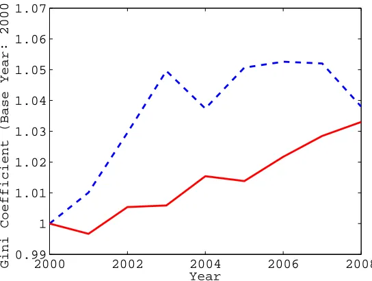
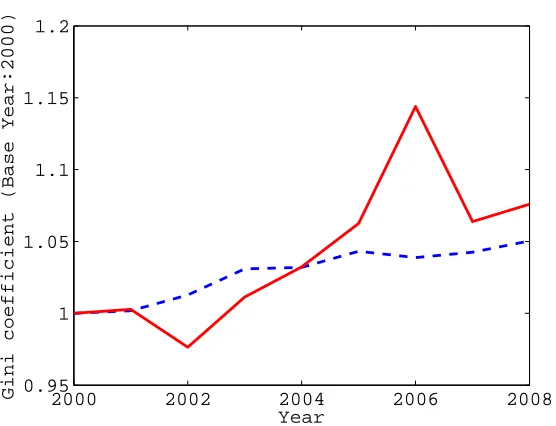
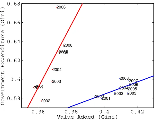
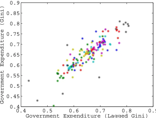
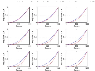
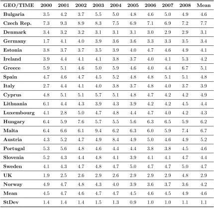
I checked therefore the Eurostat data on national accounts detailed by pro-ductive branches and I looked at the distribution of value added across different productive sectors and at the distribution of current public expenditure across sectors for European countries, and I noticed that the concentration of these dis-tributions, for example measured by the Gini coefficients of these disdis-tributions, evolve together over time. Countries that concentrate their value added over time from 2000 to 2008 also concentrate their public expenditure, while countries that diversify their value added also diversify their public expenditure. Hence, I constructed a model that interprets this correlation as a reduced form represen-tation of two structural relations. On the one hand, the distribution of public expenditure drives the future distribution of value added. On the other hand, the distribution of value added mirrors the distribution of vested interests in the economy, so that public expenditure tends to mirror the value added distribution at each point in time.
government’s budget due to these changes oppose the policy reforms, that is, the individuals working in the losing sectors oppose the reforms. The existence of political blockages of growth-enhancing reforms is not new in the literature. In fact, all the research efforts on the effects of institutions on growth focuses on the conflicting interests between the ruling elites and the rest of the population. What is new in my work is that by allowing for a proper voting process I obtain that even the majority of the population might oppose growth-enhancing reforms, so that even in perfectly functioning democratic societies it is natural to think of delays in the development path due to persistent suboptimal allocations of resources.
In Chapter 4, I look at how the transmission of shocks through the network of intersectoral linkages can originate aggregate fluctuations. The main mecha-nism through which the sectoral composition of an economy influences aggregate efficiency is the complementarity or substitutability of sector-specific value added in the composition of aggregate production. If the sectors are complementary enough, then diversification would increase aggregate efficiency, and if the sec-tors are substitutable then it’s specialization that yields higher returns. Sectoral complementarity is though a complicated object to analyze, and its connection to the moments of aggregate production is much more complex than just the long-run effect on the level of aggregate output. In fact, the complementarity among sectors depends on the input-output structure of the economy, which consists of a network of sectors supplying intermediate goods to each other. The literature has already evidenced how aggregate efficiency and aggregate volatility are tightly connected to the network structure of the economy. In particular, there are two streams of literature that explain how idiosyncratic shocks can transmit to the aggregate level and cause fluctuations of the GDP. Normally, we would expect the law of large number to apply and the idiosyncratic shocks to smooth out at the aggregate. On the one hand though, idiosyncratic shocks to firms can transmit to the aggregate level due to the size distribution of firms, that is, identical shocks to big and small firms have very different consequences to the aggregate output. On the other hand, idiosyncratic shocks to sectors transmit to the aggregate level because there are some sectors that work as hubs to the economy, that is, they supply their intermediate goods to almost all the sectors of the economy. So these sectors amplify the effect of idiosyncratic shocks making them have an effect on aggregate production.
Chapter 2
Market Structure,
Nonconvexities, and Equilibrium
Bias of Technology
As a consequence of a technological change, the productivity of a factor may increase even when its supply increases. In this paper we analyze the determinants of this technological bias. We present a general equilibrium model, where a good is produced in the final sector using both a factor and a technology, and the technology is produced in the intermediate sector. We allow for different market structures in the intermediate sector, and we prove that both competition and a variable set of technology producers may affect the occurrence of the technological bias, since they affect the necessary nonconvexities in the equilibrium allocation.
2.1
Introduction
In this paper, we look at the determinants of the so-called technological bias in a general equilibrium set-up. We relate the existence of technological bias to the presence of nonconvexities in the equilibrium allocation as in Acemoglu [3]. We prove that the market structure of the sector where the technology is produced affects the equilibrium nonconvexity and is therefore a salient feature of the technological bias.
When innovations alter the ratio of marginal products of the different factors of an economy, the technology is said to be biased. Hicks [12], Solow [16], and Acemoglu [2] are, among others, seminal works on the subject and boosted a wide empirical literature on the existence of technological bias, e.g., Goldin and Katz [11] and Autor, Katz, and Krueger [6]. If the marginal product of a factor increases when its supply increases, then, the technology is said to be biased or directed towards that factor. The rationale behind this is the endogeneity of the technological change. A factor may need a technology produced in a certain sector in order to be operative. Hence, if the supply of such a factor increases, then the factor-specific technology is more profitable. This stimulates the production of such a technology, which in turn increases the factor’s productivity. In a situation of perfect competition this causes an increase in the factor price in equilibrium. See, e.g., Acemoglu [1] for the case of skill-biased technical change and its effects on wage inequalities.
We define the technological bias as an equilibrium phenomenon, where an in-crease in a factor’s supply causes an inin-crease in its equilibrium price. The existence of technological bias is tightly connected to the presence of nonconvexities at equi-librium, that is, non-standard features of a general equilibrium allocation such as saddle points, kinks, discontinuities, and so on. We present a general equilibrium model of a two-sector economy, a final good sector and a technological sector.1
The final sector employs factors and intermediate goods in the production of a final good. The intermediate goods embody a certain level of homogeneous tech-nology, which is supplied by the firms in the technological sector.2 We distinguish
between three market structures of the technological sector. In the Benchmark Case, the technological sector is occupied by a monopolist producer that embeds the technology in the intermediate good used in the final good production. In the Cournot Case, the technological sector is populated by a finite number of firms that produce the same variety of intermediate good and compete `a la Cournot among them. In the Dixit-Stiglitz Case, a continuum of intermediate monopolistic
1
For a similar set-up, see Acemoglu [3].
2
2.2 The Benchmark Case - Economy M
firms supply different varieties of intermediate goods to the final sector.
We prove in all three set-ups that the nonconvexity of the equilibrium surface is necessary and sufficient to the existence of technological bias. We show also how such a nonconvexity depends not only on the shape of the production function but also on the set of intermediate good producers. In particular, first, we show that there exists technological bias only if the mark-ups in the technological sector are high enough. In other words, competition in the technological sector convexifies the equilibrium surface and rules out the possibility of technological bias. Second, we show that there may exist technological bias when the entry of new firms in the technological sector depends on the factor supply. In other words, an endogenous number of technology producers may entail a nonconvex equilibrium surface due to indirectly increasing returns of the factor supply.
We could list other market structures of the technological sector that would determine the occurrence of technological bias such as contestable markets, price competition with differentiated products, or price competition with capacity con-straints.3 Our results are based on a Schumpeterian approach where market power
provides the necessary incentives to endogenous and possibly biased technological change.4 We acknowledge nevertheless the alternative perspective where
com-petition for survival in highly innovative environments is the main channel of technological change.5 In fact, the two approaches refer to inherently different
industry-specific dynamics, as pointed out in Aghion et al. [4].
The paper is organized as follows. In Section 2 we simplify the framework of Acemoglu [3] and we formulate the Benchmark Case. Sections 3 and 4 provide the Cournot and Dixit-Stiglitz Cases. Section 5 draws the final conclusions. The Appendix collects all the proofs.
2.2
The Benchmark Case - Economy M
We present a simplified version of Acemoglu [3, Economy M] as the benchmark of our analysis.6 Consider a static economy, which we call Economy M, composed
of two sectors, the final good sector and the intermediate good sector. There is
3
See respectively Baumol, Panzar, and Willig [7], Salop [15], and Kreps and Scheinkman [13]. Epifani and Gancia [10] present a similar approach to ours, that is, a comparative statics exercise with different types of market structure.
4
See, e.g., Romer [14] and Aghion and Howitt [5].
5
See, e.g., Boldrin and Levine [8].
6
a unique final good, a unique intermediate good embodying a unique technology, and a unique factor of production.
The final good sector consists of a final good producer which operates under perfect competition. Since the final good is unique, the price of the final good can be normalized to one. The problem of the firm is
max
Z∈R+,q∈R+
π(Z, q |θ, w, χ) =α−α(1−α)−1[G(Z, θ)]αq1−α−wZ−χq, (2.1)
where Z ∈ R+ is the amount used of the single factor in the economy, θ ∈R+ is the scalar parameterizing the general level of the unique non-rivalrous technology, and q ∈ R+ is the quantity of the unique intermediate good, the ownership of which guarantees access to the embedded technology θ. The real-valued function
G(·,·) is twice continuously differentiable in (Z, θ) and is called the productive kernel. This function is combined with the intermediate good’s quantity q into the production function
Y =α−α(1−α)−1[G(Z, θ)]αq1−α, (2.2) so that the shares of the two subcomponentsGandqare described by the constant
α∈(0,1). The termα−α(1−α)−1 is simply a useful normalization. The element
wis the price of the factorZ and χis the price of the intermediate goodq, which are both taken as given by the firm since it operates under perfect competition. Also the level of technologyθ is exogenous to the final good firm’s problem.
The optimal quantity of the intermediate good must satisfy the first order condition (henceforth, FOC) of this problem, from which we derive a demand function for the intermediate good,
q=q(χ|Z, θ)≡α−1G(Z, θ)χ−α1, (2.3) where the demanded quantity is expressed as a function of its price χ that is influenced by the factor’s employment Z and the technological level θ.
In the intermediate good sector there is a monopolist that supplies the tech-nology to the final good firm. The monopolist sells an intermediate good that embodies the produced technology. We can think of the intermediate good as a patent that allows access to the embedded technology. The demand for the intermediate good, (2.3), is anticipated in the intermediate firm’s problem. The monopolist decides the optimal intermediate good price and the optimal level of technology. We can view technology as an innovative effort that the monopolis-tic technology provider may exert at a certain cost in order to maximize its own profits. The problem of the firm in the intermediate sector is then
max
θ∈R+,χ∈R+
2.2 The Benchmark Case - Economy M
where χq are the total revenues from the sale of the intermediate good, (1−α) is the unitary production cost of the intermediate good, and C(θ) is the cost of producing the technological level θ.7 The real-valued function C(·) is
twice-continuously differentiable. We assume that C(·) is increasing and convex in the levelθ of technology. The intermediate good firm solves the problem (2.4) subject to the demand function (2.3) for the intermediate good.
The technology menu consists of just one type of technology. Once the latter is created the technology provider can produce as many units of the intermediate good as it prefers. Each and every unit of the intermediate guarantees to the purchaser, that is, the final good firm, access to whatever level of technology is embedded in the patent. Therefore, the incentive to purchase more than just one unit of the intermediate good is the role that this intermediate asset plays in the final good production function, (2.2), rather than the level of technology embedded in it.
The unique factorZ is supplied inelastically, so the market clearing condition for the factor is
Z ≤Z,¯ (2.5)
where ¯Z ∈ R+ is the exogenous inelastic supply of the factor, and Z is the employment level, that is, the demand, chosen by the final good firm.
The optimization problems in the two sectors and the relevant market clearing condition permit us to define a concept of equilibrium for this economy.
Definition 1 (Equilibrium in Economy M.). An equilibrium is a set of firm de-cisions {Z, q}, technology level θ, intermediate price χ, and factor price w such that {Z, q} solve the problem (2.1) of the final good firm given prices{w, χ} and technology level θ, the technology level θ and the intermediate price χ solve the monopolist problem (2.4) subject to the demand (2.3) for the intermediate good, and the market clearing condition (2.5) holds.
We refer to a technology level θ at equilibrium as an equilibrium technology. The equilibrium allocations are given by the FOCs of the respective problems, under the sufficient conditions for optimality represented by the second order conditions (SOC) in each problem. We impose the following assumption, which restricts the shape of the productive kernel Gin its first argument, Z.
Assumption 1(Strict Concavity). For allθ∈R+, the functionG(·, θ) is
increas-ing and either strictly concave or exhibitincreas-ing constant returns to scale.
The functionGdoes not need to be jointly strictly concave in (Z, θ). Assump-tion 1 simply represents a sufficient condiAssump-tion for optimality in (2.1). The final
7
good firm chooses Z and the intermediate good firm chooses θ. Hence, the (Z, θ) plane is the collection of the control variables of the two agents of the economy. We are led therefore to the following solution for the equilibrium allocation.
Proposition 1 (Equilibrium-Equivalent Problem of Economy M). Suppose As-sumption 1 holds. Then, a technology level θ is an equilibrium technology if and only if θ is a solution to
max
θ∈R+FM(Z, θ)|Z= ¯Z≡G(Z, θ)|Z= ¯Z−C(θ). (2.6)
Note that, after we substitute for the optimal quantity and price of the inter-mediate good in (2.1) and (2.4), these two optimization problems have separate control spaces, since in (2.1) the control variable is Z and in (2.4) the control variable is θ. This is a key point for the results, since the separation of the op-timization problems permits the presence of nonconvexities in the overall (Z, θ) space, although not in Z or θ separately. This means that in the (Z, θ) plane there might exist saddle points, kinks, and other non-standard features of the equilibrium surface.
From now on we will call (2.6) the equilibrium-equivalent problem of Economy M, and its solution the equilibrium level of technology, θ( ¯Z). The latter depends on the level of the exogenous and inelastic factor supply, ¯Z, that is, the state variable of the whole model. We will call the objective function of (2.6), FM, the
equilibrium function of Economy M.
We substitute the equilibrium quantity and price of the intermediate good, q∗ and χ∗, inside the objective function of (2.1) and we obtain
max
Z∈R+
G(Z, θ)
1−α −wZ.
The FOC with respect to the factor’s employment yields
w∗ =w(Z, θ)
Zθ== ¯Zθ( ¯Z) ≡
(1−α)−1∂G(Z, θ)
∂Z
Zθ= ¯=Zθ( ¯Z)
, (2.7)
that is, the competitive price of the factor equals its marginal productivity for each given level of technology. Since it is computed at the equilibrium point ( ¯Z, θ( ¯Z)), we call (2.7) the factor price in equilibrium.
Suppose that w(Z, θ) is differentiable in both its arguments at the equilibrium point ( ¯Z, θ( ¯Z)) and that∂θ(Z)/∂Z exists at ¯Z. Then, we define the technological bias in the following way.8
8
2.2 The Benchmark Case - Economy M
Definition 2 (Technological Bias). There is technological bias at ¯Z if
dw(Z, θ) dZ
Zθ== ¯θZ( ¯Z)
= ∂w(Z, θ)
∂Z
Zθ== ¯θZ( ¯Z)
+ ∂w(Z, θ)
∂θ
Zθ== ¯θZ( ¯Z)
∂θ(Z)
∂Z
Z= ¯Z
>0, (2.8)
that is, if the total derivative of the equilibrium price obtained through the chain rule is locally strictly positive.
We call the first element of the total derivative the Hicksian component, and the second element the equilibrium bias component. Note that, since Assumption 1 holds, the Hicksian component is negative for all (Z, θ). Hence, a precondition for the existence of technological bias is that the equilibrium bias component is locally positive in ( ¯Z, θ( ¯Z)). We want to focus on an equilibrium phenomenon that refers to a change in the equilibrium price in absolute terms and not relative to the wage of other possible factors, that is at least locally valid at the equilibrium point ( ¯Z, θ( ¯Z)), and that consists of an equilibrium bias component strong enough to overtake the negative effect of the Hicksian component.
We can formulate a theorem that identifies a necessary and sufficient condition for the existence of technological bias in Economy M.
Theorem 1 (Technological Bias in Economy M). Consider Economy M. There is technological bias at Z¯ if and only if the Hessian ∇2
M of FM(Z, θ) is not negative
semi-definite at ( ¯Z, θ( ¯Z)).
This theorem is a reformulation of the result in [3, Theorem 4]. The failure of joint concavity of the equilibrium function and the conditions induced by the agents’ maximization problems imply the presence of technological bias.9 Since
technology and factor demands are chosen by different agents, that is, the tech-nology monopolist and the final good firm, the equilibrium allocation may not be a maximum on the entire space of both factor quantity and technology, that is, in the (Z, θ) plane. It may be instead a saddle point which results as a maximum of FM only separately in the control spaces of the final good firm, that is, in
the factor quantity Z, and of the monopolist, that is, in the technology level θ. The economy’s equilibrium set-up originate the nonconvexity, not the productive technologies of the agents. Thus, if we change the market relations, we affect the nonconvexity and therefore the possibility of technological bias. The claim of the present work is that the market structure plays a key role in the formation of nonconvexities in equilibrium, and therefore in the existence of technological bias.
9
Note that in order to have FM jointly concave in (Z, θ) at the equilibrium point ( ¯Z, θ( ¯Z)),
its Hessian with respect to (Z, θ),∇2
M, should necessarily be negative semi-definite at this point,
2.3
The Cournot Case - Economy Q
In this section we present a model that casts a link between the Benchmark Case and the perfect competition case in the technological sector. This is important in order to determine why technological bias is not compatible with high levels of competition.
Consider a two-sector economy, called Economy Q, where there is unique firm in the final good sector operating under perfect competition and N firms in the technological sector that compete in quantities `a la Cournot. There exists a unique type of nonrival technology. Moreover, we assume that the intermediate goods where the technology is embedded are perfectly substitutable.
The final good firm’s problem is
max
Z∈R+,Q∈R+
π(Z, Q|θ, χ) =α−α(1−α)−1[G(Z, θ)]αQ1−α−wZ−χQ, (2.9) where Q represents the quantity of intermediate goods employed by the final good firm. The intermediate good’s price χis the equilibrium result of a Cournot interaction in the intermediate sector. We apply to (2.9) the FOC with respect to
Qand obtain the total demand for intermediates, which we express as an inverse demand function, that is,
χ=χ(Q|Z, θ)≡α−α[G(Z, θ)]αQ−α, (2.10) where θ is again the technology to which the final good firm has access.
Let N be the number of technology producers, and let n indicate the generic producer, that is,n= 1, ..., N. Each technology producer supplies its own quantity of intermediate goodqnand provides its own technology levelθn. Since technology
is unique and nonrival, the technology level to which the final good firm has access,
θ, is the maximum among the levels provided by all the technological producers, that is,
θ= max{θn}Nn=1. (2.11) Each intermediate producer solves the same symmetric problem, that is,
max
θn∈R+,qn∈R+
Πn(θn, qn |χ(Q|Z, θ)) = (χ−(1−α))qn−C(θn), (2.12)
where qn is the individual quantity, χ the intermediate price, and θn the
firm-specific technology production. The control variables of the technology producers are different from (2.4), since now firms choose the optimal quantity and the price is determined by the market clearing. The factor market clears when (2.5) holds. The market clearing condition for the intermediate goods market is instead
Q≤ N
X
n=1
2.3 The Cournot Case - Economy Q
that is, total demand of intermediate goods is equal to total supply. We can formulate a definition of equilibrium in Economy Q that is similar to the definition of equilibrium in Economy M.
Definition 3 (Equilibrium in Economy Q). An equilibrium in Economy Q is a set of firm decisions {Z, Q, q1, ..., qN}, technology levels {θ1, ..., θN} and θ,
inter-mediate price χ, and factor price w such that θ solves (2.11), {Z, Q} solve the problem (2.9) of the final good firm given prices{χ, w}and technology θ,{θn, qn}
solve the problem (2.12) of the n-th intermediate good firm for any n∈ {1, ..., N}
given (2.10), and the market clearing conditions (2.5) and (2.13) hold.
On the one hand, since the demand for intermediate goods depends on the maximum among all the technology productions, each technology producer has the incentive to free ride on the technology production of the other providers. So the symmetric solution for which all firms produce the maximal technology is not a (Nash) equilibrium. On the other hand, the solution where all the firms produce a nil technology is not an equilibrium either, since each firm in this case would make zero profits while producing some technology and stimulating a nonnil demand for the intermediate goods would yield stricly positive profits, even if shared with the competitors. Hence, if one of the technology producers, with probability 1/N, decides to produce a nonnil amount of technology, then everybody gains, although the actual producer pays all the costs of technology production. The other technology providers produce a nonnil level of technology as well, since otherwise the final good firm has no incentive to buy their intermediate goods. At the margin, the actual producer wants to produce the amount of technology that maximizes its profits, no matter how much profit the other free-riding competitors realize. Thus, it maximizes its how profit function regardless of the others. There exists N asymmetric pure strategy equilibria. All of them yield the same maximal technology, θ. The following proposition characterizes the equilibrium technology.
Proposition 2 (Equilibrium-Equivalent Problem of Economy Q). Suppose As-sumption 1 holds. Then, a technology level θ is an equilibrium technology if and only if θ is a solution to
max
θ∈R+
FQ(Z, θ)|Z= ¯Z ≡
Ω(N, α)
N2 G(Z, θ)|Z= ¯Z−C(θ), (2.14)
where
Ω(N, α)≡
N −α N(1−α)
1−αα
The intuition is that (2.14) implies that the higher the number of intermediate good producers, N, the lower the individual share in aggregate demand and the higher the competition, and therefore the lower the incentive for the single firm to embed technology in the intermediate good. An increase in the number of firms reduces technology production. This has consequences on the existence of the technological bias. According to Definition 2, there exists technological bias only if the total derivative of the factor price is positive. The number of firms in the technological sector reduces the incentives for technology production and lowers therefore the equilibrium bias component of the total derivative. This means that, even though technology increases as the factor supply increases, it may not increase enough to compensate the negative Hicksian effect on the factor price.
We substitute for the equilibrium level of Qand χin (2.1) and we obtain
max
Z∈R+
Ω(N, α)
1−α G(Z, θ)−wZ.
Hence, the factor price in equilibrium
w(Z, θ)
Zθ== ¯θZ( ¯Z) ≡
Ω(N, α) 1−α
∂G(Z, θ)
∂Z
Zθ== ¯θZ( ¯Z), (2.16)
where Ω(N, α) is defined in (2.15).
The following theorem states the equivalence between equilibrium nonconvex-ity and technological bias in this economy.
Theorem 2 (Technological Bias in Economy Q). Consider Economy Q. There is technological bias in Economy Q at Z¯ if and only if the Hessian ∇2
Q of FQ(Z, θ)
is not negative semi-definite at ( ¯Z, θ( ¯Z)).
The technological bias is incompatible with low individual incentives to tech-nology production. The high number of firms affects the potential nonconvexity of the equilibrium, that is, it makes the equilibrium function’s Hessian negative semi-definite.
Corollary 1 (Technological Bias and Number of Firms in Economy Q). Suppose Assumption 1 holds. If
G(Z, θ)
C(θ)
Zθ== ¯θZ( ¯Z)
> ∂
2G(Z, θ)
∂θ2
Zθ== ¯θZ( ¯Z) −
(∂2G(Z, θ)/∂Z∂θ)2
(∂2G(Z, θ)/∂θ2)C′′(θ)
Zθ= ¯=Zθ( ¯Z)
, (2.17)
then, there exists a number N of firms high enough such that the technology pro-ducer’s profits are nonnegative and
dw(Z, θ) dZ
Zθ== ¯θZ( ¯Z)
2.4 The Dixit-Stiglitz Case - Economy DS
The intuition behind (2.17) is the following. On the one hand, technology producers make nonnegative profits at equilibrium only if
N2
Ω(N) ≤
G(Z, θ)
C(θ)
Zθ= ¯=θZ( ¯Z)
,
where G(Z, θ)/C(θ) is a measure of the monopolistic mark-up. If the number of firms, N, is too high, the mark-up cannot be enough for all the participants to make positive profits. On the other hand, the total derivative of the factor price in equilibrium is negative when
N2
Ω(N) >
∂2G(Z, θ)
∂θ2
Zθ= ¯=Zθ( ¯Z) −
(∂2G(Z, θ)/∂Z∂θ)2
(∂2G(Z, θ)/∂θ2)C′′(θ)
Zθ== ¯θZ( ¯Z)
,
that is, when the joint concavity of the equilibrium surface is strong enough. The element on the right hand side measures both the joint concavity of the production kernel, G, and the convexity of the cost function, C. First, the more concave the production with respect to the factor, the stronger the Hicksian effect, and therefore the more likely the total derivative to be negative. Second, the more concave the production with respect to the technology, the less the increase in demand due to technology production. Third, the higher the production cross-effects between the factor and the technology, the higher the interaction between factor supply and technology availability. And fourth, the more convex the cost function, the more costly are increases in technology. There is technological bias only if this element is low with respect to the number of firms. Hence, if the mark-up and the joint concavity of the equilibrium solution are high enough, there exists a number of firms such that the equilibrium bias is not enough to compensate the Hicksian effect. If the mark-up was too low, a few additional firms in the technological sector would imply already negative profits. If the joint concavity was moderate, the technological bias would disappear only with a high number of firms.
The Cournot case bridges the Benchmark Case with the presence of competi-tion. In fact, whenN = 1 we are back to Economy M. This fills a gap in Acemoglu [3], where only the dichotomic difference between perfect competition with no bias and monopoly with bias is analyzed. Economy Q permits to map the effect of competition on firms’ profits and consequently on the technological bias.
2.4
The Dixit-Stiglitz Case - Economy DS
Acemoglu [3, Economy O] than Economy Q, in order to rule out the possibility of negative profits with high levels of competition. This is important in order to characterize the effects of a variable set of technology producers on the existence of technological bias.
Consider a two-sector economy, called Economy DS, where there is a unique firm in the final good sector operating under perfect competition and the inter-mediate sector is populated by a continuum of massN of symmetric intermediate firms. Each firm is the monopolistic producer of a specific intermediate good, and the unique final good firm combines the entire range of intermediate goods in its production function according to a symmetric level of substitutability. All the firms produce the same type of technonogy.10
The final good firm uses a production function `a la Dixit and Stiglitz.11 Hence,
its problem is
max
Z∈R+,{qj}j∈[0,N]
α−α(1−α)−1[G(Z, θ)]α
Z N 0
qj1−αdj−wZ−
Z N 0
χjqjdj, (2.18)
where j is the continuous type index, [0, N] is the range of available types, qj is
the quantity produced by the j-th technology provider, χj is its price, θ is the
type-independent level of technology, and 1−α represents the substitutability of the intermediate goods in the final good production. The FOCs of (2.18) with respect toqj yield a demand function for every intermediate type j that depends
on the priceχj of that intermediate, that is,
qj =q(χj |Z, θ)≡α−1G(Z, θ)χ
−1 α
j . (2.19)
The monopolistic intermediate producer of typej maximizes its own profits sub-ject to the intermediate good-specific demand expressed by the final good firm. We suppose symmetry among intermediate producers. Thus, the problem of the
j-th monopolist is
max
θn,χj
Πj(θn, χj |q(χj |Z, θ)) = (χj−(1−α))qj −C(θn), (2.20)
subject to (2.19). The market clearing condition for the factor is given by (2.5). We define the equilibrium in Economy DS in a similar way to the definition of equilibrium in Economy M and Economy Q.
10
The case for firm-specific technology types corresponds to [3, Economy O]. The only conse-quence is on the equilibrium-equivalent problem, while our main results would not change.
11
2.4 The Dixit-Stiglitz Case - Economy DS
Definition 4 (Equilibrium in Economy DS). An equilibrium in Economy DS is a set of firm decisions {Z,{qj}j∈[0,N]}, technology levels {θj}j∈[0,N] and θ, factor
price w, and intermediate prices {χj}j∈[0,N] such that {Z,{qj}j∈[0,N]} solve the
problem (2.18) of the final good firm given prices {w,{χj}j∈[0,N]}and technology
θ,θj andqj solve the problem (2.20) of thej-th monopolist subject to the demand
(2.19) for every j ∈ [0, N], (2.11) holds, and the market clearing condition (2.5) is satisfied.
The existence and uniqueness of the maximal produced technology is in line with Economy Q. If the technology type was firm-specific and not unique, the equilibrium technology would be the fixed point of a mass N of maximization problems.12 This would not affect our results below.
Proposition 3 (Equilibrium-Equivalent Problem in Economy DS). Suppose As-sumption 1 holds. Then, a technology level θ is an equilibrium technology if and only if θ is a solution to
max
θ∈R+
FDS(Z, θ)|Z= ¯Z ≡G(Z, θ)|Z= ¯Z−C(θ). (2.21)
The problem in (2.21) coincides with (2.6), since it is the result of a massN of symmetric monopolistic problems. Proposition 3 is different from Proposition 2 because the numberN of competitors does not enter the profits of the intermediate firms.
We substitute the equilibrium quantities and prices of the intermediate goods into (2.18) and obttain
max
Z N(1−α)
−1G(Z, θ)−wZ.
We then impose the FOC and obtain the factor price in equilibrium, that is,
w(Z, θ)
Zθ== ¯θZ( ¯Z) ≡
N
1−α
∂G(Z, θ)
∂Z
Zθ= ¯=Zθ( ¯Z)
. (2.22)
The mass of technological firms, N, enters the equilibrium price of the factor because there exists a love for variety of inputs in the production of the final good. This means that the higher the mass N, the higher the final production. While in Economy Q the number of firms enters also the profit function of the technology producer, (2.14), in Economy DS the mass of firms enters only the
12
factor price. Note that the degree of input substitutability, parameterized by 1−α, is the inverse of the mark-up, 1/(1−α). Thus, the more substitutable the intermediate goods, the lower the incentive to technology production, as we can see in (2.22).
Theorem 3 (Technological Bias in Economy DS). Consider Economy DS. There is technological bias at Z¯ if and only if the Hessian ∇2
DS of FDS(Z, θ) is not
negative semi-definite at ( ¯Z, θ( ¯Z)).
Since every technology producer is a monopolist in the production of the in-termediate good, the equivalence between equilibrium nonconvexity and existence of technological bias is the same as in Economy M. Theorem 3 holds for every ex-ogenousN.
We propose a new set-up of Economy DS where the mass of firms is an in-creasing function of the amount of the aggregate factor.
Assumption 2. The mass N of firms is an increasing function of the amount Z
of the aggregate factor, that is,
N =N(Z), (2.23)
where N′(Z)>0 for every Z ∈R
+.
Since the profits of the technology producers do not depend on the level of competition, firm entry does not depend on any nonnegative-profits requirement. Hence, Assumption 2 is compatible with the rest of the set-up.
Remark. Note that the amount Z of the aggregate factor in (2.23) is not the control variable of the perfectly competitive final good firm. In fact, we can think of a mass 1 of symmetric final good firms under perfect competition, where each firm i chooses its firm specific employment Zi and aggregate factor demand is
Z ≡ R1
0 Zidi, with the market clearing condition R1
0 Zidi ≤ Z¯. Hence, the single
firm i does not control Z. We skip this notation for simplicity.
If Assumption 2 holds, then the total derivative of the equilibrium price of the factor has an additional element. This implies that we need to redefine the technological bias.
Definition 5 (Technological Bias with a Variable Number of Technology Produc-ers). There is technological bias at ¯Z if
dw(Z, θ, N) dZ
Zθ= ¯=Zθ( ¯Z)
= ∂w(Z, θ, N)
∂Z
Zθ= ¯=Zθ( ¯Z)
+
+∂w(Z, θ, N)
∂θ
Zθ= ¯=Zθ( ¯Z)
∂θ(Z)
∂Z
Z= ¯Z
+
+∂w(Z, θ, N)
∂N
Zθ= ¯=Zθ( ¯Z)
∂N(Z)
∂Z
Z= ¯Z
>0,
2.4 The Dixit-Stiglitz Case - Economy DS
that is, if the total derivative of the equilibrium price obtained through the chain rule is locally strictly positive.
The third element of the total derivative is positive as long as Assumption 2 holds and the factor price is given by (2.22). Hence, although the Hicksian component was bigger than the equilibrium bias component, the third component could add enough bias so as to make the total derivative positive.
Theorem 4 (Technological Bias with a Variable Number of Technology Pro-ducers). Consider Economy DS. Suppose that Assumption 2 holds. Then, there is technological bias at Z¯ if the Hessian ∇2
DS of FDS(Z, θ) is not negative
semi-definite at ( ¯Z, θ( ¯Z)).
The failure of equilibrium joint concavity in the (Z, θ) plane is only a sufficient condition for the existence of technological bias when Assumption 2 holds. There may exist the technological bias also if the third element of the total derivative of the factor price is high enough. We propose hereafter a characterization of Economy DS where there is technological bias although the production kernel is jointly concave.
the pharmaceutical firm hires to produce medicines coincides with the number of researchers N that give their innovations to the firm for private profit, that is,
N =Z.
Suppose that the productive kernel G has a Cobb-Douglas form satisfying As-sumption 1, e.g.,
G(Z, θ) =Zǫθ1−ǫ,
withǫ∈(0,1). Moreover, suppose that technology production costs are quadratic, that is,
C(θ) =θ2/2.
Then, the factor price is
w(Z, θ)
Zθ== ¯θZ( ¯Z)
= N 1−αǫZ¯
ǫ−1θ( ¯Z)1−ǫ. (2.25)
The equilibrium level of technology is the solution of (2.21), that is,
θ(Z) = (1−ǫ)1+1ǫZ ǫ 1+ǫ.
Moreover, N =Z and at equilibrium Z = ¯Z, so the total derivative is
dw(Z, θ) dZ
Nθ==θZ( ¯= ¯ZZ)
= 2ǫ
2(1−ǫ)11+−ǫǫ
(1−α)(1 +ǫ)Z¯
ǫ−1 1+ǫ >0.
On the one hand, there exists technological bias. On the other hand, the deter-minant of the Hessian of the equilibrium functionFDS at equilibrium is
∇ 2 DS Zθ== ¯θZ( ¯Z)
=ǫ
¯
Z
1−ǫ
−1+2ǫ
>0,
that is, the Hessian of FDS is negative definite. Hence, there is technological bias
even if the equilibrium is jointly concave in the (Z, θ) plane.
2.5 Conclusion
2.5
Conclusion
In this paper we have investigated the determinants of the technological bias. We show that the technological bias exists when the equilibrium surface is nonconvex. We cast a link between the market structure of the technological sector and the existence of the nonconvexities in equilibrium. We compare the Benchmark Case of monopoly in the technological sector with two alternative settings. In the Cournot Case we show that technological bias is incompatible with high levels of competition. In the Dixit-Stiglitz Case we claim that if the set of active firms in the technological sector depends on the factor supply, the technological bias may occur even when the equilibrium surface is jointly concave in the factor employment and the technology. We provide an example that characterizes the claim.
An implication of our model is that, if we want to include a technological bias mechanism in, e.g., a growth model, we can simply control for the market structure of the technological sector or the entry decision of the technological producers. We do not need to impose assumptions on the aggregate production function. Moreover, in a structural regression, if the technological bias is an endogenous regressor, we need an instrument for it. Our model proposes the market structure of the technological sector as a theoretically consistent instrument. This suggests an empirical application of Acemoglu [3]’s results.
Our model fills a gap in Acemoglu [3]. Economy Q encompasses both the monopoly case of [3, Economy M] and the competition case. It shows how the equilibrium nonconvexity depends on the market structure, due to the effect of competition on the technology producers’ incentives. Economy DS analyzes the case where the set of technological firms depends on the factor employment. This helps us understand how the size effect of an increase in the factor supply may influence the factor prize.
Our analysis of the existence of equilibrium bias in presence of alternative mar-ket structures is similar to Epifani and Gancia [10]. Nevertheless, they diversify the market structure of the final good sector while we focus on the technologi-cal sector. We consider similar market structures, that is, imperfect competition frameworks where the agents alternatively compete in quantities or provide firm-specific intermediate goods. Their conclusions about the relation between the existence of scale bias and the level of competition are the same as ours, although they deal with relative bias while we concentrate on absolute bias.
position of the increased factor with respect to others. The social condition of a factor may deteriorate even in the presence of absolute technological bias once we allow for an increase in the factor supply. What we would need for a welfare improvement of the increasing factors is augmenting or at least factor-specific technologies. Furthermore, we can argue that redistributing the gains given by the increase in total factor productivity induced by the technological bias would yield Pareto-improving increases of factor supplies.
An important area of future research is an empirical test of the structural relations implied by the present work. For instance, in a setting of increasing factor supply, we could test whether increasing or decreasing factor prices are correlated with changes in the market structure of the technological sector.
2.6
Appendix: Proofs
Proof of Proposition 1. Since Gis increasing in Z under Assumption 1 and (2.5) holds, the optimal level of employment for the factor is the border solution Z∗ =
¯
Z. Therefore, the FOC with respect to the quantity of intermediate good q is, according to (2.3),
q(χ|Z, θ)
Z= ¯Z =α
−1G(Z, θ)
|Z= ¯Zχ−
1 α.
We substitute q into the monopolist problem (2.4), that is,
max
θ∈R+,χ∈R+
(χ−(1−α))α−1G(Z, θ)
Z= ¯Zχ
−1
α −C(θ).
The FOC with respect toχyields χ∗ = 1. We plug this into the demand function and obtain
q(χ|Z, θ)
Zχ= ¯=1Z =α
−1G(Z, θ)
Z= ¯Z.
We substitute the values for the intermediate good’s equilibrium price and quan-tity into (2.4), that is,
max
θ∈R+
=G( ¯Z, θ)−C(θ).
Proof of Theorem 1. The function FM(·,·) in (2.6) is twice continuously
differen-tiable in (Z, θ), since both G(·,·) and C(·) are twice continuously differentiable. Since Assumption 1 holds,
∂FM(Z, θ)
∂Z =
∂G(Z, θ)
∂Z and
∂2FM(Z, θ)
∂Z2 =
∂2G(Z, θ)
2.6 Appendix: Proofs
We impose the FOC and the SOC on (2.6) and obtain
∂FM(Z, θ)
∂θ
Zθ== ¯θZ( ¯Z)
= 0 and ∂
2F
M(Z, θ)
∂θ2 Zθ= ¯=Zθ( ¯Z)
<0. (2.26)
First, the function ∂FM(·,·)/∂θ is a mapping from R2+ to R+. Second, it is
lo-cally C1. Third, its value is zero at the equilibrium point ( ¯Z, θ( ¯Z)). Fourth, its
derivative with respect to the θ, ∂2F
M(·,·)/∂θ2, is not nil at equilibrium because
of the SOC. Hence, we satisfy all the hypotheses of the Implicit Function Theorem (IFT) and we can apply it to the FOC of (2.6), (2.26), that is,
∂θ(Z)
∂Z
Zθ== ¯θZ( ¯Z)
=−
∂(∂FM(Z, θ)/∂θ)
∂Z
∂(∂FM(Z, θ)/∂θ)
∂θ Zθ= ¯=θZ( ¯Z)
=−
∂2F
M (Z, θ)
∂Z∂θ ∂2F
M (Z, θ)
∂θ2 Zθ= ¯=Zθ( ¯Z)
.
However,
∂w(Z, θ)
∂Z = (1−α)
−1∂2G(Z, θ)
∂Z2 = (1−α)
−1∂2FM(Z, θ)
∂Z2 ,
and
∂w(Z, θ)
∂θ = (1−α)
−1∂2G(Z, θ)
∂Z∂θ = (1−α)
−1∂2FM(Z, θ)
∂Z∂θ .
Hence, we can rewrite (2.8) as
dw(Z, θ) dZ
Zθ= ¯=Zθ( ¯Z)
= (1−α)−1
"
∂2F
M(Z, θ)
∂Z2 −
(∂2F
M(Z, θ)/∂Z∂θ)2
∂2F
M(Z, θ)/∂θ2
# Zθ== ¯Zθ( ¯Z)
>0.
The Hessian of FM is
∇2M =
∂2F
M(Z, θ)/∂θ2 ∂2FM(Z, θ)/∂θ∂Z
∂2F
M(Z, θ)/∂θ∂Z ∂2FM(Z, θ)/∂Z2
.
Since (2.26) holds,, ∇2
M is not locally negative semi-definiteness if
∂2F
M(Z, θ)
∂θ2
Zθ== ¯θZ( ¯Z) ×
∂2F
M(Z, θ)
∂Z2 Zθ== ¯θZ( ¯Z)
<
∂2F
M(Z, θ)
∂θ∂Z
Zθ== ¯θZ( ¯Z)
2
,
that is, if
∂2F
M(Z, θ)
∂Z2 Zθ== ¯θZ( ¯Z)
> (∂
2F
M (Z, θ)/∂θ∂Z)2
∂2F
M(Z, θ)/∂θ2
Zθ== ¯θZ( ¯Z)
Suppose that ∇M(Z, θ) is not locally negative semi-definite. Then, since (1−
α)−1 >0,
dw(Z, θ) dZ
Zθ== ¯θZ( ¯Z)
>0,
that is, there is technological bias.
Conversely, suppose that the Hessian ofFM is negative semi-definite at ( ¯Z, θZ¯).
Then,
∂2F
M(Z, θ)
∂θ2
Zθ= ¯=θZ( ¯Z) ×
∂2F
M(Z, θ)
∂Z2
Zθ== ¯θZ( ¯Z) ≥
∂2F
M(Z, θ)
∂θ∂Z
Zθ= ¯=θZ( ¯Z)
2
.
But (2.26) holds, so
dw(Z, θ) dZ
Zθ== ¯θZ( ¯Z) ≤
0,
that is, there is no technological bias.
Proof of Proposition 2. Since Assumption 1 and (2.5) hold, Z∗ = ¯Z. Then, from (2.13) and (2.10) we obtain that
χ=α−α[G(Z, θ)|Z= ¯Z]α N X n=1 qn !−α .
Thus, the individual intermediate problem,
max
θn,qn
α−α[G(Z, θ)|Z= ¯Z]
α N X n=1 qn !−α
−(1−α)
qn−C(θn)
yields the following FOC with respect toqn,
qn(χ|Q) =Q
χ−(1−α)
αχ =q.
Hence, the optimal quantity of the intermediate good,q, is symmetric. The market clearing condition (2.13) becomes
Q=
N
X
n=1
q=Nq.
We substitute for this value in the FOC above and obtain the equilibrium price for the intermediate,
χ∗ = N(1−α)
2.6 Appendix: Proofs
Thus, the optimal individual quantity of the intermediate is
q(χ|Z, θ)
χZ== ¯χZ∗
=
N−α N(1−α)
α1
G(Z, θ)|Z= ¯Z
αN ,
which implies that
Q(χ|Z, θ)
χZ== ¯χZ∗
=
N −α N(1−α)
α1
G(Z, θ)|Z= ¯Z
α
We plug these values in (2.12) to obtain
max
θn
N −α N(1−α)
1−αα
G(Z, θ)|Z= ¯Z
N2 −C(θn).
Since there exist N asymmetric pure strategy equilibria (see discussion in Section 2), the maximum level of available technology, θ, is equivalent to the solution of the above problem for some n in{1,· · · , N}.
Proof of Theorem 2. The functionFQ(·,·) is twice continuously differentiable. Since
the factor price in equilibrium is given by (2.16),
∂w(Z, θ)
∂Z
Zθ= ¯=θZ( ¯Z) =
Ω(N) 1−α
∂2G(Z, θ)
∂Z2
Zθ== ¯θZ( ¯Z) =
N2
1−α ∂2F
Q(Z, θ)
∂Z2
Zθ== ¯θZ( ¯Z),
and
∂w(Z, θ)
∂θ
Zθ= ¯=θZ( ¯Z) =
Ω(N) 1−α
∂2G(Z, θ)
∂Z∂θ
Zθ== ¯θZ( ¯Z) =
N2
1−α ∂2F
Q(Z, θ)
∂Z∂θ
Zθ== ¯θZ( ¯Z).
We apply the IFT to the FOC of (2.14), which yields
∂θ(Z)
∂Z
Zθ= ¯=Zθ( ¯Z)
=−∂
2F
Q(Z, θ)/∂Z∂θ
∂2F
Q(Z, θ)/∂θ2
Zθ== ¯θZ( ¯Z)
.
We substitute the relations above into the total derivative of (2.16) and obtain
dw(Z, θ) dZ
Zθ== ¯θZ( ¯Z)
= N
2
1−α
"
∂2FQ(Z, θ)
∂Z2 −
(∂2FQ(Z, θ)/∂θ∂Z)2
∂2F
Q(Z, θ)/∂θ2
# Zθ== ¯θZ( ¯Z)
.
Hence, the failure of negative semi-definiteness of the Hessian of FQ, ∇2Q, is a
Proof of Corollary 1. According to (2.14), the profits of the actual technology producer at equilibrium are nonnegative if and only if
Ω(N, α)
N2 G(Z, θ)−C(θ)
Zθ== ¯Zθ( ¯Z) ≥
0,
for any N, that is,
N2
Ω(N, α) ≤
G(Z, θ)
C(θ)
Zθ== ¯θZ( ¯Z)
.
We can rewrite the total derivative of the factor price as
dw(Z, θ) dZ
Zθ== ¯Zθ( ¯Z)
= Ω(N) 1−α
∂2G(Z, θ)
∂Z2 +
∂2G(Z, θ)
∂Z∂θ
∂θ(Z)
∂Z
Zθ== ¯θZ( ¯Z)
,
that is,
dw(Z, θ) dZ
Zθ= ¯=Zθ( ¯Z)
= Ω(N) 1−α
∂2G(Z, θ)
∂Z2 −
∂2G(Z, θ)
∂Z∂θ
2
∂2G(Z, θ)
∂θ2 −
N2
Ω(N)C ′′(θ) Zθ= ¯=θZ( ¯Z)
.
Hence, the total derivative is negative if and only if
N2
Ω(N, α) >
∂2G(Z, θ)
∂θ2
Zθ== ¯θZ( ¯Z) −
(∂2G(Z, θ)/∂Z∂θ)2
(∂2G(Z, θ)/∂θ2)C′′(θ)
Zθ= ¯=Zθ( ¯Z).
Proof of Proposition 3. From Assumption 1 and (2.5) we setZ∗ = ¯Z. Hence, the demand for the j-th intermediate good is
qj(χj |Z, θ)|Z= ¯Z =α−1G(Z, θ)|Z= ¯Zχ
−α1
j ,
for all j ∈[0, N]. The j-th intermediate firm solves (2.20) subject to the demand above. The FOC with respect to the j-th intermediate good price, χj, yields the
symmetric equilibrium price for the intermediate good χ∗
j = 1, for all j ∈[0, N].
We substitute the intermediate price into the intermediate demand and obtain
qj(χj |Z, θ)
χZ= ¯Z
j=1
=α−1G(Z, θ)|Z= ¯Z =q,
for all j ∈[0, N]. The problem (2.20) is then equivalent to
max
θj