NOISE SOURCE DETECTION USING NON-ORTHOGONAL MICROPHONE ARRAY

NOISE SOURCE DETECTION USING NON-ORTHOGONAL

MICROPHONE ARRAY

43.50.YW INSTRUMENTATION AND TECHIQUES FOR NOISE MEASUREMENT AND ANALYSIS

Fujita, Hajime1; Fuma, Hidenori1; Katoh, Yuhichi1; and Nobuhiro Nagasawa2 1

Department of Mechanical Engineering, College of Science and Technology, Nihon University 1-8 Kanda Surugadai, Chiyoda-ku, Tokyo 101-8308 Japan

Tel/Fax: +81-3-3259-0738

e-mail: fujita@mech.cst.nihon-u.ac.jp

2

Hitachi Advanced Systems, Corp.

216 Totsuka-cho, Totsuka-ku, Yokohama, Kanagawa 244-8567 Japan Tel: +81-45-881-1221

Fax: +81-45-862-2063

e-mail: nobuhiro_nagasawa@cm.as.hitachi.co.jp

ABSTRACT

Microphone array for noise source detection usually consists of two straight arrays arranged in cross or X shape. When multiple noise sources of nearly same levels are present, however, 2 arrays systems often show “ghosts” of the real source images. Three straight arrays are arranged here with the crossing angle of 60 degrees each other, named as “Star- array” in order to avoid the ghosts. Numerical simulation and experimental study for both stationary and moving noise sources proved that newly developed Star-array depressed the ghosts down to non-detectable level.

INTRODUCTION

advantage over the cross-type array for the noise source measurement in horizontally distributed noise sources such as in high-speed train, because the side lobes of the source image appear along array lines. However, as long as only two arrays are used for multi-noise source measurement, the problems of the so-called ghosts of the source image cannot be avoided. The main purpose of this paper is to demonstrate the performance of the array system with three non-orthogonal arrays to avoid the ghosts, by numerical simulation and experiments.

THE SOURCE IMAGES AND GHOSTS

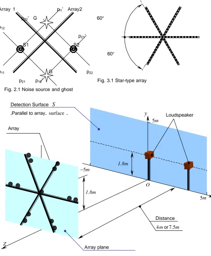
A single straight array shows the location of the noise source along the line perpendicular to the array. In Fig. 2.1, the images of the source S1 appear along the line p11 - p11’ for array 1 and along the line p12 - p12’ for array 2. Similarly, the images of S2 appear on lines p21 - p21’ and p22 - p22’. The true images of these noise sources appear at the crossing points S1 and S2. However, the ghosts, marked by G with stars also appear at the crossing points of these lines. If, however, one more array is added properly as shown in Fig. 3.1, the true source locations will appear at the crossing point of three image lines. Since there are no other points where three image lines coincide except the true source location, the ghosts will not appear at the crossing points of two image lines.

EXPERIMENTAL APPARATUS

Each microphone array used in experiments has 21 independent microphones with the spacing of 170 mm, with the central microphone common to all three arrays as shown in Fig. 3.1. The arrays are crossing each other at the angle of 60° and the array center is located at 1.8 m above the ground. Two loudspeakers, 3 m apart, are placed in front of the arrays, 4 m or 7.5 m from the array plane as shown in Fig. 3.2. For moving noise source measurements, a car with two loudspeakers runs in front of the array at the speed of 20 km/h or 80 km/h as shown in Fig. 3.3. Sound barriers and absorbers are used to avoid the effect of the tire noise and the reflection of the noise emitted from the loudspeakers, as shown in Fig. 3.4. The microphone signals are recorded on 64 ch. digital recorder and are analyzed off line with a PC in the laboraotry.

RESULTS

Numerical Simulation

The comparison of the noise source images reproduced by the X-array and Star-array using numerical simulation is shown in Fig. 4.1. The true noise sources are located at (0, 0) and (3, 0) on x-y plane. The X-array shows the ghosts at (1.5, 1.5) and (1.5, -1.5) in addition to the true source images. On the other hand, the Star-array is free from the ghosts. Thus the validity of the Star-array is proved by numerical simulation.

The resolutions of the Star-array for single noise source located at various positions are shown in Fig. 4.2. The values obtained by numerical simulation well agree with the experimental values. Figure 4.3 and 4.4 show the experimental results of the detection of two equal level noise sources located at (0, 1.8) and (3, 1.8) at 7.5 m and 4 m from the array plane, respectively. At these distances, the sound wave emitted from the loudspeaker cannot be considered as a plane wave, and spherical wave corrections are adopted for reconstruction of the noise source images. At 7.5 m, two noise sources show almost equal level and the 2nd source at (3, 1.8) shows a little wider peak width. At 4 m, the peak widths are smaller than those of 7.5 m, however, the level of the 2nd source seems to be 1.5 dB smaller than the 1st one. This is due to the difference in the distances between the source and the center of the array, which can be corrected. There are some side lobes of -6 to -5dB at the location of the ghost but are distinguishable from the true images.

Experiments for Moving Noise Sources

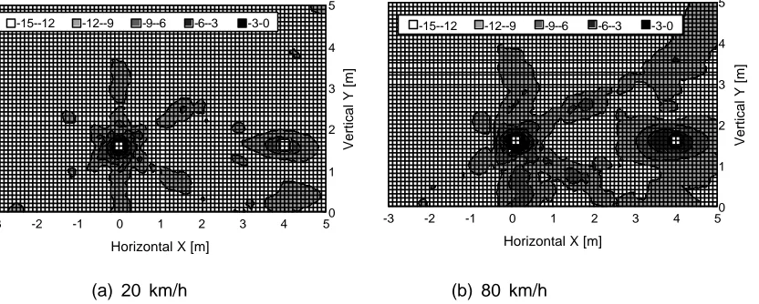
Two loudspeakers of equal noise level are attached to the car as shown in Fig. 3.3 and the experiments are performed for two car speeds, 20 km/h and 80 km/h. The results are shown in Figs. 4.5 and 4.6. The noise source locations are at (0, 1.6) and (4, 1.6) and are marked with the white squares in the figures. The accuracy of the noise source locations is satisfactory for the car running at 7.5 m from the array surface, but is rather poor for the rear noise source of the car running at 4 m. This is due to the increase of the distance between the soude and the array center and the increase of the incident angle of the sound to the array. The accuracy will become even for front and rear sources if the data are analyze when the sources are located at (-2, 1.6) and (2, 1.6).

CONCLUSIONS

The experimental results of the resolutions of the array are very close to the theoretical values obtained by numerical simulation. The arrangement of the Star-array effectively eliminated the ghosts of the noise source images both for stationary and moving dual noise sources of equal strength effectively. The cost of Star-array is the total length of the array, which is directly affecting the resolution. Technical and economical balance must be taken into account for actual applications.

REFERENCES

Array 1 p11’ Array2

p22’ G 60° p12

p21’ S1 S2

60°

p11 G p22

p21 p12’ Fig. 3.1 Star-type array Fig. 2.1 Noise source and ghost

Fig. 3.2 Microphone arrays and stationary noise sources

4000 mm Loudspeaker Array

900 mm h h

2330 mm h=1600 mm 1600 mm Sound absorber 700 mm Sound barrier

Fig. 3.3 Moving noise sources on a car Fig. 3.4 Moving noise measurement 60

=

γ

− =

γ

=

γ

m

Array plane

Distance m

4 or7.5m

m 5 m

5 −

x

y

Z

m 5

O 1.8m

Detection Surface

S

Array

1.8m

(a) X array with ghosts (b) Star array without ghost Fig. 4.1 comparison of array types for appearance of ghosts

0 0.2 0.4 0.6 0.8 1 1.2 1.4 1.6 1.8 2

0 1 2 3 4 5

Horizontal X(m)

Resolution (m)

Äx Simulation7.5m Äy Simulation7.5m

Äx Simulatioin4m Äy Simulation4m

Äx Measured7.5m Äy Measured7.5m

Äx Measured4m Äy Measured4m

4.2 Resolution of single noise source

(a) Front view (b) Side view

Fig. 4.3 Separation of two stationary noise sources at 7.5 m

-5 -4 -3 -2 -1 0 1 2 3 4 5

5 4 3 2 1 0 -1 -2 -3 -4 -5

Horizontal X [m]

Vertical Y [m]

-15--12 -12--9 -9--6 -6--3 -3-0

-5 -4 -3 -2 -1 0 1 2 3 4 5 5 4 3 2 1 0 -1 -2 -3 -4 -5

Horizontal X [m]

Vertical Y [m]

-15--12 -12--9 -9--6 -6--3 -3-0

-2 -1 0 1 2 3 4 50

1 2 3 4 5

Horizontal X [m]

Vertical Y [m]

-15--12 -12--9 -9--6 -6--3 -3-0

-2 -1 0 1 2 3 4 5 -15 -12 -9 -6 -3 0 Response(dB) Horizontal X(m)

(a) Front view (b) Side view Fig. 4.4 Separation of two stationary noise sources at 4 m

(a) 20 km/h (b) 80 km/h Fig. 4.5 Separation of two moving noise sources at 7.5 m

(a) 20 km/h (b) 80 km/h Fig. 4.6 Separation of two moving noise sources at 4 m

-2 -1 0 1 2 3 4 50

1 2 3 4 5

Horizontal X [m]

Vertical Y [m]

-15--12 -12--9 -9--6 -6--3 -3-0

-2 -1 0 1 2 3 4 5

-15 -12 -9 -6 -3 0

Response(dB)

Horizontal X(m)

-15--12 -12--9 -9--6 -6--3 -3-0

-3 -2 -1 0 1 2 3 4 50

1 2 3 4 5

Horizontal X [m]

Vertical Y [m]

-15--12 -12--9 -9--6 -6--3 -3-0

-3 -2 -1 0 1 2 3 4 50

1 2 3 4 5

Horizontal X [m]

Vertical Y [m]

-15--12 -12--9 -9--6 -6--3 -3-0

-3 -2 -1 0 1 2 3 4 50

1 2 3 4 5

Horizontal X [m]

Vertical Y [m]

-15--12 -12--9 -9--6 -6--3 -3-0

-3 -2 -1 0 1 2 3 4 50

1 2 3 4 5

Horizontal X [m]

Vertical Y [m]