ACOUSTIC ASSESSMENT OF A STEERING WHEEL SENSOR USING PARTICLE VELOCITY METHOD

ACOUSTIC ASSESSMENT OF A STEERING WHEEL SENSOR USING PARTICLE

VELOCITY METHOD

PACS:43.58FM

Luís Figueiredo1_{, Marco Dourado}1_{, Seyyed M.M. Sabet}1_{, António Pereira}1_{, Francisco Pinto}2_{, Irene Brito}3_,

José Machado1_{, José Meireles}1_{, Castor Rodríguez Fernández}4

1_{MEtRICs Research Center, School of Engineering, University of Minho;}

Campus de Azurém da Universidade do Minho, 4800-058 Guimarães, Portugal E-Mail: {lfigueiredo, mdourado, sabet, b7043, jmachado, meireles}@dem.uminho.pt;

2_{Bosch Car Multimedia S.A;}

Rua Max Grundig, 35, Lomar, 4705-820 Braga, Portugal E-Mail: [email protected];

3_{Center of Mathematics, School of Sciences, University of Minho;}

Campus de Azurém da Universidade do Minho, 4800-058 Guimarães, Portugal E-Mail: [email protected];

4_{Sound of Numbers SL}

A Coruña, Spain

E-Mail: [email protected]

Keywords:

Steering wheel sensor (LWS), Noise assessment, Particle velocity method, Scan and Paint

ABSTRACT

Noise generation in modern vehicles cabin is mainly due to the contact among small mechanical parts integrated on systems such as steering angle sensors. Currently, to ensure that the noise produced by the steering angle sensors is below the limits, it is necessary to carry out tests in an anechoic environment. This work aims to compare the steering angle sensors produced by two different ways (normal line production in factory and 3D printer technology) using a PU probe with a particle velocity and pressure sensor, as well as a software for graphical noise display (Scan and Paint feature). This method is shown to be less susceptible to the surrounding environment noise as compared to the conventional microphones and it can be used in the assembly line for noise assessment of steering angle sensors.

RESUME

INTRODUCTION

Currently, the assessment of the acoustic behavior of automotive components is done using microphones in an anechoic environment. However, since having an anechoic chamber in the production line is almost impossible, it is necessary to use an alternative technique to evaluate the acoustic behavior of this components in the production line, as for example the Scan & Paint technology [1].

The control and regulation of external noise produced by vehicles dates back as late as 1929. The maximum noise limit from 82dB (A) in 1978 was reduced to 74dB (A) in 1996 and based on regulations in the European Union in 2014; this limit is to be set to 68dB (A) by 2026 [2]. Noise reduction inside the car cockpit is important since the tendency of the automotive industry is to increase the number of electric vehicles and there is a growing demand for cars with quieter cabins where small components such as the steering wheel angle sensors (LWS), contribute to the general acoustic behaviour of the cockpit [3]. The LWS is a sensor that measures the angle, position and rotation speed of the steering wheel. The measurements from LWS sensor, together with the information of other sensors, are used to control various driving assistance systems, such as electronic stability control, steering power and active steering control [4].

There is a significant interest in developing tools to assess the sound behaviour by qualitative and quantitative ways. The representation of sound has been the subject of many studies to provide an intuitive and a better visual understanding of each specific case study [5]. The sound visualization technique called “Scan and Paint” is based on manually moving a transducer across a measurement plane while filming the process by a camera placed perpendicular to the measurement [6] [7]. The position of the sensor is then obtained by applying automatic colour detection in each frame during the post-processing stage. Depending on the position of the probe, each fragment of the signal is linked to a grid cell [8].

The integration of "Scan & Paint" feature into the particle velocity measurement technique allows a visual acoustic analysis of LWS sensor. Since the particle velocity sensor ignores most of the background noise, it can be used in the production line. The combination of these two technologies allows visual identification of the locations with higher sound density (e.g. holes in the structure), high noise transmission zones, as well as PVL (Particle Velocity Level) at each frequency [1].

Viscardi et al used the Scan & Paint method and particle velocity sensor to design and test a light-weight foam [9]. Rowe et al [10] used a scanning sound intensity and particle velocity sensor to optimize and reduce the noise radiation of an unmanned aerial vehicle (UAV). Guiot et al [11] applied the Scan & Paint method and the particle velocity sensor to assess the acoustic intensity of a turbo-compressor system. Comesana et al [12] used a particle-velocity probe based on scanning method to characterize the acoustic behaviour of a loudspeaker. Other researchers [13] [14] used the Scan & Paint feature and particle velocity sensor to study the sound leakage inside the car cabin.

This paper presents the noise assessment of a steering wheel sensor, LWS, using microphones as an initial step, and then a scanning measurement technique (Scan & Paint) coupled with a particle velocity sensor for a detailed analysis. This work is dedicated to the acoustic analysis of six LWS sensors of identical geometry. Five sensors were obtained directly from the production line and the sixth one produced by additive manufacturing (3D printing). The only difference between the 3D printed sensor and the others is the polymer type and its surface finish.

THEORICAL CONCEPTS

Sound can be described as an auditory sensation, which is produced by the ear's reaction to transient or oscillatory variations of pressure in relation to atmospheric pressure. Generally, it is possible to describe the sound as the displacement of a mechanical wave that propagates through air or other elastic medium. This displacement is caused by the movement of air molecules through actions of elastic stress involving the compression and expansion of the medium through which it is propagating. This propagation results from the transmission of the movement of some molecules to the neighbouring molecules and so on, by means of which oscillation of the vibration propagates through the medium to our ears. Although the human ear only detects the pressure variations that occur in relation to atmospheric pressure, the sound waves are composed by the pressure variation and the particles velocity oscillation [15] [16].

It can be seen from Figure 1 that acoustic pressure and particle velocity are not in phase in the near field and even if both magnitudes can be measured with transducers at the same time, they provide different quantities of sound level.

Figure 1 - Acoustic pressure and particle velocity variation for a pure tone in the near field (adapted from [17]).

As it can be seen in Figure 1, where the pressure is maximum, the particle velocity variation is zero and when the particle velocity variation is maximum, the pressure variation is zero. Therefore, when measuring very close to a surface that is vibrating (emitting sound) the particle velocity values of that surface have its maximum variation and the particle velocity values from background noise is zero because the pressure variation for background noise is at maximum. [17].

Sound involves a wide range of pressures and, normally, a logarithmic scale is used for frequencies and the decibel scale to measure sound levels. The sound pressure level (SPL) is presented in equation (1), where p is the measured acoustic pressure and the reference value for the acoustic pressure, pref, is equal to 2*10-5 _Pa.

(1)

The particle velocity level (PVL) is given by equation (2) where v is the measured particle velocity and the reference value for the particle velocity, vref,, is equal to 5*10-8 _m/s.





















ref

p

p

(2)

The human ear has weak sensibility at low and high frequencies, so a filter, commonly referred as the A-weight, has been defined, which adjusts the noise level measured values (dB) to the sensibility of the human ear [18].

The particle velocity sensor from Microflown is based on MEM’s technology (micro electromechanical systems), having dimensions of about 1mm wide, 2mm long and 300μm thick. The resistive thin wires used to measure the particle velocity have a width of 10μm and a thickness of 200nm. The particle velocity measurement is done through two platinum resistive thin wires heated to 200 ° C, as presented in Figure 2 [16].

Figure 2 - Resistive wires connected to the electrical connectors and the Microflown sensor assembled on a printed circuit board (PCB) [16].

The two resistive wires are crossed by a certain electric current, heating up to 200 ºC by Joule effect. If there are no particles passing through the wires, there is only heat transfer from the wires to the surroundings through natural convection. When an air flow passes through the hot thin wires, they will cool due to heat transfer by forced convection. The first wire will cool more than the second wire, and due to the difference of temperature between the two wires, it is possible to measure the particle velocity [16] [19] [20]. As the temperature of the materials directly influences its electrical resistance, it will generate a difference of voltage, proportional to the particle velocity of the air (airflow) that passes through the wires. It is also possible to know the direction of the airflow by observing and identifying the wire at the lowest temperature. When measuring a sound wave, the air flow (particle velocity) alternates according to the shape of the sound wave, generating an alternating voltage in the sensor [16] [19]. This is the main advantage in the directionality of this type of sensor in relation to the microphone.

LWS SENSOR

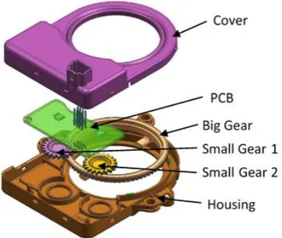
The LWS sensor consists of 6 different components, as shown in Figure 3. The structure of the sensor is composed of a housing and a cover. Inside LWS sensor there is a gear system containing two small gears and a larger one that is driven by the steering column of the vehicle and a PCB board which measures the steering information while driving.





















ref

v

v

Figure 3 - The assembly of a LWS sensor

The noise can be transmitted in two ways: structure-borne or air-borne noise transmission [21]. Structure-borne noise transmission is generated by a structure whose vibration is transmitted to the neighbouring structures. Air-borne noise transmission is generated by a vibrating surface moving the air molecules, creating a progressive movement of the air particles that spread and impact in our eardrum. In the LWS sensor, the noise is transmitted by both ways. The rotation of the gears and impact of the teeth promote the structural vibration of the components (structure-borne), which subsequently excites the air molecules inside the sensor to vibrate causing air-borne [22].

EXPERIMENTAL METHODOLOGY

Six functional sensors, with identical geometry and components shown in Figure 3, were used for the experimental studies. Five of these sensors were obtained directly from the production line, while the sixth sensor was produced by 3D printing (housing and cover). The sensor produced by 3D printer is composed of a different material and surface finish from the other five sensors, which is expected to produce a different acoustic behavior.

The first test was performed with two microphones in an anechoic environment. Each microphone allow studying the acoustic behavior of each sensor in the frequency spectrum of 1/3-octave bands. The two microphones were placed axially and radially in relation to the sensor at a distance of 200 mm. Each experimental test was based on an average of three consecutive measurements.

In the second test the measurements were performed using Microflown particle velocity sensor with the Scan & Paint feature [22]. The measurements were performed in the lower part of the housing and cover, at a distance of approximately 1 cm. This allows visual representation of areas with high and low particle velocity levels (PVL).

EXPERIMENTAL RESULTS

The 5 sensors obtained from the production line are referred as "Sensor O" 1 to 5, while the 3D printed one as "3D Printer". The sound pressure level (SPL) at 1/3 octave band spectrum between 100Hz and 10 kHz is shown in Figure 4.

Figure 4 - One-third octave band graph obtained by the horizontal microphone.

It can be found, from Figure 4, that the 3D printed sensor produces higher noise at all frequencies compared to the production ones. It can also be seen that the dominant frequency of the 3D printed sensor is 1000 Hz, in contrast with 3150 Hz for the other five sensors. The 1/3 octave spectrum is nearly the same for the five sensors with only 3 dB difference in total RMS acoustic sound between the noisiest and quietest sensor, calculated using the formulation to add several decibel values [23].

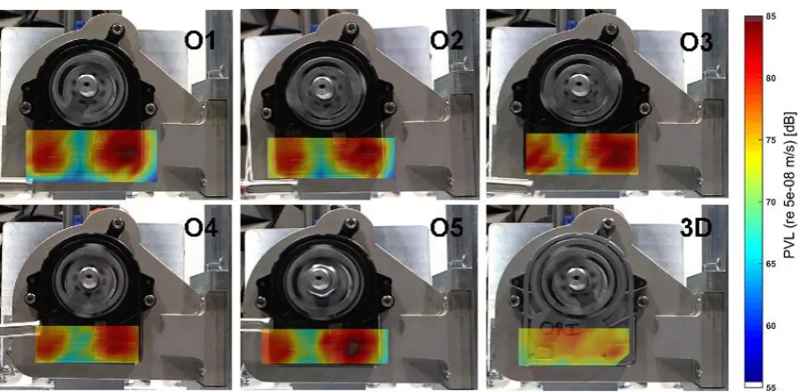
In the second set of tests, measurements were made and PVL intensity maps are shown at 500 Hz and 3150 Hz for the lower housing part of the sensor, in Figures 5 and 6, respectively.

Figure 5 - PVL visualization on the housing of O1 to O5 and the 3D printed sensors at 500 Hz.

100 1000 10000

SPL[

d

b

(A)

]

Frequency [Hz]

Sound Pressure Level (SPL)

Sensor O1

Sensor O2

Sensor O3

Sensor O4

Sensor O5

Figure 6 - PVL visualization on the housing of O1 to O5 and the 3D printed sensors at 3150 Hz. One can observe from Figures 5 and 6 that PVL pattern for the production sensors is similar between them at both frequencies. However, the 3D printed sensor shows a distinctly different PVL pattern in both frequencies when compared to the production line sensors. It was therefore concluded that the noise behaviour of the 3D printed sensor is different from the other five sensors.

Figures 7 and 8 show PVL intensity maps for the 3D printed and production sensors at 500 Hz and 3150 Hz frequencies for the lower cover part of the sensor, respectively.

Figure 8 - PVL map of O1 sensor (left) and the 3D printed one (right) performed on the cover at frequency of 3150 Hz.

It can be seen from comparing Figures 7 and 8 with Figure 5 and 6, that the PVL patterns are different on the housing and cover. This is due to the fact that the two parts have different geometries and that the gears and PCB board are placed on the housing (and not cover). Similarly, the PVL pattern of a 3D printed sensor is different when compared with the production sensors.

Figure 9 shows the PVL graphs obtained from the housing while Figure 11 illustrates the graphs from the cover. PVL graphs in Figure 9 were drawn by interpolation of points throughout the 1/3 octave band frequency spectrum.

Figure 9 – PVL graphs for O1 to O5 and 3D printed sensors obtained from the housing. It can be seen from Figure 9 that the 3D printed sensor has a higher PVL level throughout the frequency range, indicating that it is noisier than the other five, as shown in Figure 4. The PVL peaks of the 3D printed sensors are at 250 Hz, 1000 Hz and 2500 Hz, while those of O sensors are observed at 250 Hz, 500 Hz and 1600 Hz. The PVL level can be used as an index to identify a defective sensor,

40 45 50 55 60 65 70 75

100 1000 10000

PVL

[d

B]

Frequency [Hz]

Particle Velocity Level (PVL)

Sensor O1

Sensor O2

Sensor O3

Sensor O4

Sensor O5

shown in Figure 10, was defined.

Figure 10 – Measurement points on the cover of O1 and 3D printed sensors.

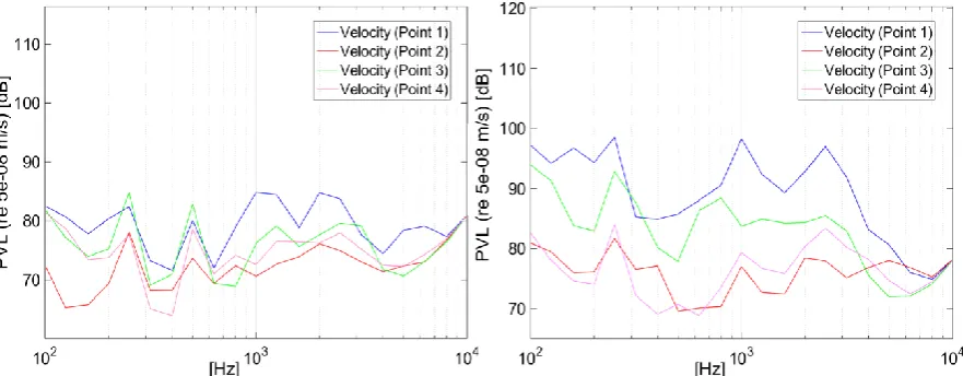
Figure 11 shows the PVL graphs for the four points on O1 (left) and 3D printed sensor (right). It can be seen from Figure 11 that, similarly to the measurements on the housing (Figure 9), the 3D printed sensor has a higher PVL intensity than O1 sensors. Point 1 in both graphs in Figure 11 represents the highest PVL, and Point 2 shows the second highest PVL intensity. The most prominent frequency peaks of O1 sensors are observed at 250 Hz and 500 Hz for all points, and at 1000 Hz, 1250 Hz, 2000 Hz and 2500 Hz for point 1.

Figure 11 – PVL graphs of O (left) and 3D printed (right) sensors obtained from 4 points. The main frequency peaks for the 3D printed sensor can be found at 250 Hz and 2500 Hz for all points, while it is 800 Hz for point 2 and 1000 Hz for points 1, 3 and 4. As mentioned earlier, the difference between the two sensors can be observed through the PVL levels and/or the frequencies at which PVL peaks are placed.

CONCLUSIONS AND FUTURE WORK

This work is based on acoustic analysis of LWS sensors by means of Scan & Paint and the particle velocity sensor for local noise assessment (identification). Initially, acoustic measurements were performed using microphones in an anechoic chamber on five sensors obtained from the production line as compared to a 3D-printed one, and it was shown that the 3D printed sensor has a higher noise level. Then the same analysis was performed using Scan & Paint and particle velocity sensor to obtain

Point 1

Point

2

Point

3

PVL patterns. By obtaining PVL graphs and the frequencies at which PVL peaks occur, one may easily identify a defective sensor. The analysis can be performed either on an area or a specific set of critical points. Since this technique is not affected by ambient noise, it can be used to compare the acoustic behavior of the LWS sensors in the production line.

As of future work, the Scan & Paint and particle velocity technology is to be implemented in the LWS sensor assembly line to assess the acoustic behavior of the sensors and to detect the production defects such as the absence of a component.

ACKNOWLEDGMENT

This work was sponsored by the Portugal Incentive System for Research and Technological Development. Project in co-promotion nº 002797/2015 (INNOVCAR 2015-2018).

REFERENCES

[1] D. F. Comesaña, S. Steltenpool, G. P. Carrillo, H. E. d. Bree and K. R. Holland, Scan and Paint: Theory and practice of sound field visualization method, International Scholarly Research Notices, 2013.

[2] VCA Offices, “Noise,” UK Vehicle Type Approval Authority, 2017 03 15. [Online]. Available: http://www.dft.gov.uk/vca/fcb/cars-and-noise.asp. [Accessed 2017 03 15].

[3] M. Jóźwicka, “Electric vehicles: moving towards a sustainable mobility system,” European Environment Agency, 14 11 2016. [Online]. Available: http://www.eea.europa.eu/articles/electric-vehicles-moving-towards-a. [Accessed 2017 03 16].

[4] HUNTER Engineering Company, “What you need to know about - Steering Angle Sensors and Alignment Service,” June 2013. [Online]. Available: https://www.pro-align.co.uk/wp-content/uploads/2016/05/6158T-Steering-Angle-06-13.pdf. [Accessed 16 03 2017].

[5] R. T. Beyer, “Sounds of Our Times,” in Two Hundred Years of Acoustics, Berlin, Germany, 1999. [6] H. E. d. Bree, J. Wind, E. Tijs and A. Grosso, Scan & Paint, a new fast tool for sound source

localization and quantification of machinery in reverberant conditions, 2010.

[7] E. Tijs, H.-E. d. Bree and S. Steltenpool, “Scan & paint: a novel sound visualization technique,” in Proceedings of the 39th International Congress and Exposition on Noise Control Engineering (Inter-Noise '10), 2010.

[8] D. F. Comesaña, “Mapping stationary sound fields [M.S. thesis],” Institute of Sound and Vibration Research, 2010.

sound intensity p-u probe to optimize and reduce the noise radiation of an UAV developed for cinematography,” Internoise2016, 2016.

[11] M. Guiot, D. F. Comesana, M. Korbasiewicz and G. C. Pousa, “Turbo-compressor and piping noise assessment using a particle velocity based sound emission method,” Internoise2015, 2015.

[12] D. F. Comesana, A. Grosso and K. R. Holland, “Loudspeaker cabinet characterization using a particle-velocity based scanning method,” AIA-DAGA Conference on Acoustics, 2013.

[13] A. Grosso, H. d. Bree, S. Steltepool and E. Tijs, “Scan & paint for acoustic leakage inside the car,”

SAE International, 2010.

[14] D. F. Comesana, A. Grosso, E. d. Bree and J. Wind, “Further Development of Velocity-based Airborne TPA: Scan & Paint TPA as a Fast Tool for Sound Source Ranking,” SAE International,

2012.

[15] H.-E. d. Bree, The Microflown E-Book, Netherlands: Microflown Technologies - Charting sound fileds, 2009.

[16] R. Raangs, Exploring the use of the Microflown, Ipskamp, Enschede: PrintPartners, 2005. [17] The Penn State University, “Air Pressure Levels vs. Air Particle Velocity Levels,” 2016. [Online].

Available: http://www.personal.psu.edu/meb26/INART50/pressureVsVelocity.pdf. [Accessed 26 07 2017].

[18] L. Figueiredo, M. Dourado, S. M. Sabet, A. Pereira, J. Machado, J. Meireles, I. Brito and F. Pinto, “Acoustic Simulation of a Steering Sensor for Geometric Design Optimization,” ICE 2017 – 23rd International Conference on Engineering, Technology and Innovation, 2017.

[19] H.-E. d. Bree, “An Overview of Microflown Technilogies,” Acta Acustica united with Acustica, pp. 163-172, 2003.

[20] Microflown Technologies, Charting sound fileds, Netherlands: Microflown Technologies, 2014. [21] J. S. Bolton and R. W. Bono, “Airborne Sound Transmission into Vehicle Cabins Through Door

Like Structures,” Proceedings of 13th International Modal Analysis Conference -Going Beyound Modal Analysis, 1995.

[22] P. Flores and J. Gomes, Ginemática e Dinâmica de Engrenagens: Aspetos Gerais sobre Engrenagens (in Portuguese), Guimarães: Escola de Engenharia - Univesidade do Minho, 2014. [23] J. P. Guyer, P.E., R.A., F. ASCE and F. AEI, “Fundamentals of Acoustics,” 2009. [Online].

Available: