Aeroacoustics analysis o single jets with noise suppression devices

FIA2008-A085

Aeroacoustics

a

nalysis

o

s

ingle

j

ets

w

ith

n

oise

s

uppression

d

evices

Bernardo Aflalo (a), bernardo.aflalo@embraer.com.br Odenir de Almeida(a), odenir.almeida@embraer.com.br

João Barbosa(a), barbosa@ita.br

(a) Centro de Referência em Turbinas a Gás, Departamento de Energia, Instituto Tecnológico de Aeronáutica. Praça Marechal Eduardo Gomes, 50, São José dos Campos, Brasil.

Abstract

Aircraft noise is a subject of great concern. This is supported by the extremely rigid aircraft noise certification process and airports regulations, allied to the increasing environment concern. The noise generated by an aircraft can be divided into two components: the airframe and the engine noise. The latter is the most important noise source during the aircraft take-off and is greatly affected by the jet noise. The goal of this work is to simulate numerically the noise of a single jet under the influence of noise suppression devices known as chevrons. Nozzles with different lobes number have been analyzed, in order to identify its influence on the dynamic and acoustic results. Chevrons are largely used in modern turbofan engines, due to the substantial jet noise reduction allied with a very low weight and performance penalty. The commercial software CFD++ has been used to obtain the

steady flow properties using RANS through a cubic k-ε turbulence model. The CAA++ aeroacoustics

tool has been used to calculate the pressure fluctuation at a far-field observer based on a random flow generation technique. The results lead to good agreement with previous works in the literature, so that it is expected that the developed methodology could be applied to the study of newly design gas turbine exhaust system aiming at reduction of jet noise.

Resumen

1 Introduction

The noise radiated by aircraft’s jet has diminished greatly in the last 40 years, because of the huge research effort in this subject, although it is still the major source of aircraft noise during the take-off. With the introduction of the turbofan engines in the aeronautical market in the 70’s, the noise has reduced greatly due to the bypass flow embracing the main core, which reduces the shear stress between the primary jet (high velocity) and the outer stream (low velocity). In the sequence, many attempts have been made to reduce the jet noise, but usually the devices have prohibitive weight or performance penalty. The position of the engine also affects the noise radiation. Installing the jet exhaust over the airplane wing would reflect most of the noise upwards. However, this concept would cause other problems, like difficult maintenance. Callender and Gutmark (2005) have stated that the use of chevrons can significantly reduce the noise produced by the jet without compromising the aircraft performance and cost.

The jet noise prediction methods available today include semi-empirical methods, experimental methods and computational methods. The first one is an essential tool to give fast results with fewer input parameters. Unfortunately, it is not adequate for the prediction of noise reduction observed in the noise suppression devices, like chevrons. The experimental methods can give good results for a large range of jet temperature ratio, Mach numbers and nozzle geometry, but they are difficult to use and usually very expensive. For these reasons, the computational methods are becoming very popular for this kind of analysis.

The acoustics phenomena of noise generation and propagation in a turbulent jet can be completely described by the Navier-Stokes equations. A large number of works have been focused on the use of more direct methods, like DNS and LES, to calculate the noise sources coupled with acoustics analogies to propagate this disturbance to the farfield. These techniques may give very good results, but the associated computational costs are still prohibitive for industrial applications. That is why a great effort is now turning to stochastic methods.

The goal of this study is to investigate the noise reduction produced by different chevron geometries using a computational aeroacoustic tool available in the commercial code CFD++, which is a stochastic model having as input a RANS flow calculation result, which reduces significantly the computational effort. Due to the relative low computational cost associated, this method is being exhaustively used in the aerospace industry for jet noise prediction applications. Two specific objectives are investigated. The first is to prove that the use of the CFD++ aeroacoustics tool can predict the effects of chevrons in the acoustics. The second is to investigate what is the effect of chevron lobe numbers in the acoustic response. Three nozzles were studied: BN00 (baseline), CN12 (chevron with 12 lobes) and CN08 (chevron with 8 lobes).

2 Problem description

The baseline simulation consists of a jet with Reynolds number of order , based on jet velocity at nozzle exit plane and nozzle diameter. The Mach number is 0.75, the jet diameter is 0.05 m (approximately 1/10 of the jet exhaust of a small turbofan aircraft), the total temperature ratio is 1 and the ambient has the following properties: the pressure is 101300 Pa, the temperature is 288 K and the medium is at rest. Even though the small dimensions of the jet nozzle, scaling procedures (Viswanathan, 2008) can be applied to estimate real size jet noise. The CN08 and CN12 nozzles simulations have the same setup, but

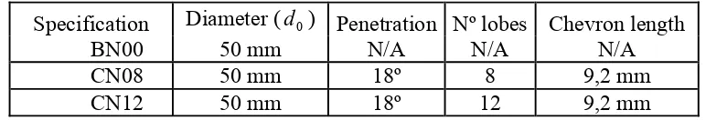
with the chevrons installed at the nozzle trailing edges. Table 1 summarizes the chevrons characteristics.

Table 1. Nozzles Characteristics.

Specification Diameter (d0) Penetration Nº lobes Chevron length

BN00 50 mm N/A N/A N/A

CN08 50 mm 18º 8 9,2 mm

CN12 50 mm 18º 12 9,2 mm

Nozzle trailing edge thickness is zero. Since the ambient flow is at rest, the metal sheet thickness would not affect the dynamic and acoustic response.

2.1 Fluid Dynamic Model

RANS simulations were first performed to obtain the flow mean characteristics. Cubic k-ε model was used because it can provide enough information for the acoustic model within CFD++. The compressible viscous simulations were performed with an implicit scheme and a ramped CFL number. The domain has been initialized in the following way: near the nozzle exit and inside a cylinder with a length of 30 and a radius of (where is the radius of the baseline nozzle), the mesh has been initialized with the jet properties. The full domain includes 100 downstream and 15.2 upstream the nozzle exit plane.

0

r r₀ r₀

0

r r₀

The boundary condition at nozzle wall is the adiabatic non-slip condition. The y+ throughout the nozzle was kept bellow unit, in such a way that wall functions are not needed. This was done to avoid the sudden change in the mathematical model (wall law/cubic k-ε

model) near the nozzle exit plane. This transition could cause an error that would mostly affect the high frequency region of the noise spectrum.

The residual plots have indicated that 2000 iterations were enough to assure a good convergence for all simulations. Due to the symmetry of the problem, only one forth of the geometry was modeled. After the RANS simulation, the mesh and the mean flow properties have had to be extrapolated to a full 360º model, in order to run the acoustic tool. Fortunately, there is no need to do this procedure with the entire domain, because the acoustic model only needs the region responsible for the noise generation, i.e. the cells with a minimum turbulent kinetic energy level. So, only this noise source region is extrapolated to full 360º.

2.2 Acoustic Model

Smirnov et al (2001) developed a random flow generation technique (RFG) to estimate the unsteady characteristics of a flow based on a RANS results.

Basically, the method consists of scaling and orthogonal transformations applied to a transient velocity field obtained by the superposition of harmonic functions. The inputs for this technique are the correlation tensor of the original flow-field and information on length and time-scales of turbulence.

software CFD++, has a modified version of this method (Batten et al, 2004). The formulation used in this simulation is represented in equation (1).

∑

i p d x t q d x t

N a t x v 1 ] ˆ ˆ ˆ sin( ) ˆ ˆ ˆ cos( [ 2 ) ,

( ω ω (1)

where τ τ π π L V c V d d t t l x

x nj _n

n j j

j = = , ˆ = , =

2 ˆ , 2

ˆ (2)

) 1 , 1 ( , 2 1 , 0 ) 1 , 0 ( , , N N d N n n i n n i n i ∈ ⎟ ⎠ ⎞ ⎜ ⎝ ⎛ ∈ ∈ ω ω ξ ς (3) n m n j ijm n i n m n j ijm n i n k n k n m n l m l n d q d p d d d d u u

c = , =ε ς , =ε ξ

2 ' ' 3 (4) ) , (x t

v_i is the velocity fluctuation of a specific element in the mesh.

2.3 Mesh Adopted

A structured mesh was implemented for this application, since previous works have related that unstructured meshes can produce inaccurate results, as related by Page et al (2002).

An extensive mesh sensibility test was carried out. For each geometry, three different meshes were tested, the first one with , the second with and the third with

cells. The results showed that for the round nozzle, the first mesh with

cells would be enough to capture the mean characteristics of the flow. For the chevron nozzles, a more refined mesh is needed. The mesh with cells has been chosen for all the nozzles, due to the goods results attained. Figure 1 shows a close up of the final mesh near the nozzle.

6 10 7 .

0 × 6

10 3 . 1 × 6 10 0 .

2 × _0.7×106

6 10 3 . 1 ×

(a) (b) (c)

2.4 Nozzle exit profile verification

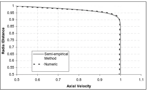
To assure a correct profile at nozzle exit, an upstream segment of the nozzle of 7.6 length was simulated and the profile was compared with semi-empirical inlet profiles present in the literature. Freund (2001) have shown a method to estimate the nozzle exit profile for a turbulent jet: 0 d ⎥ ⎥ ⎦ ⎤ ⎢ ⎢ ⎣ ⎡ ⎥ ⎦ ⎤ ⎢ ⎣ ⎡ ⎟⎟ ⎠ ⎞ ⎜⎜ ⎝ ⎛ − − = r r r r t b Uj u ₀ 0 1( , ) tanh

1 2

1 _θ

(2)

where u is the axial velocity component, Uj is the maximum jet velocity, r is radial

distance and b₁(θ,t) is 12.5. As can be seen in figure 2, the nozzle exit velocity profile is in good agreement with the methods available in the literature.

0.5 0.55 0.6 0.65 0.7 0.75 0.8 0.85 0.9 0.95 1

0.5 0.6 0.7 0.8 0.9 1 1.1

Axial Velocity R a di a l D is ta nc e Semi-empirical Method Numeric

Figure 2. Comparison between numerical and semi-empirical nozzle exit profile.

3 Results

3.1 Aerodynamic

Andersson et al (2005) carried out a LES simulation of a nozzle similar to the BN00 and compared with experimental results. The experimental data have been compared with the resulted RANS simulation, as shown in figure 3.

Axial distribution of u

0 0.2 0.4 0.6 0.8 1 1.2

0 5 10 15 20

Figure 3. Comparison between axial velocity for RANS/ Experimental data.

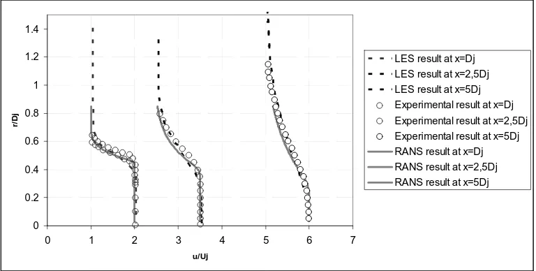
The RANS result has indicated a lengthier potential core, when compared with the experimental results. Previous works available in literature also have reported potential discrepancies between the k-ε model and experimental data (Kenzakowski, 2005). Birch (2006) has changed the k-ε model by switching the value of the Pr number near the end of the potential core. This modification in the turbulence model has adjusted the flow in a way that the turbulence level near the end of the potential core resulted in better agreement with the experimental data. The radial distribution of u is shown is the figure 4.

0 0.2 0.4 0.6 0.8 1 1.2 1.4

0 1 2 3 4 5 6 7

u/Uj

r/

D

j

LES result at x=Dj LES result at x=2,5Dj LES result at x=5Dj Experimental result at x=Dj Experimental result at x=2,5Dj Experimental result at x=5Dj RANS result at x=Dj RANS result at x=2,5Dj RANS result at x=5Dj

Figure 4. Radial Distribution of axial velocity (u) for RANS/LES/Experimental data.

The results in figure 4 show a very good agreement between the RANS results and the data gathered from Birch (2006). Even though the potential core length had not been precisely captured by the RANS simulation, the cross-section axial velocity distribution validates the dynamic result.

The following figures show the contour of the Mach and Turbulent Kinetic Energy for three different sections.

(a) BN00 (b) CN08 (c) CN12

(a) BN00 (b) CN08 (c) CN12

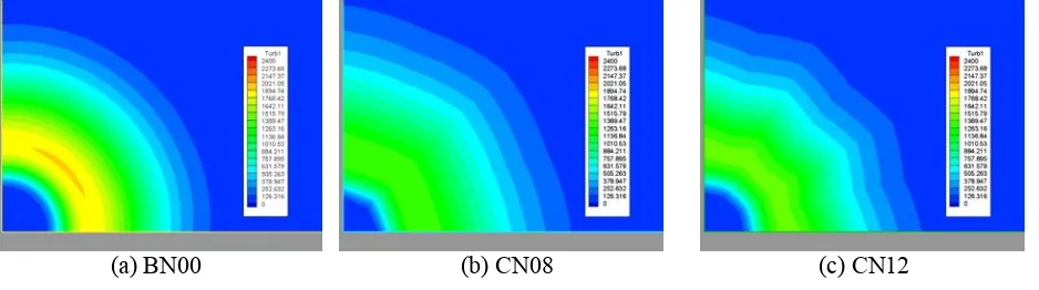
Figure 5. k contour at x=Dj.

(a) BN00 (b) CN08 (c) CN12

Figure 6. Mach contour at x=2,5Dj.

(a) BN00 (b) CN08 (c) CN12

Figure 7. k contour at x=2,5Dj.

(a) BN00 (b) CN08 (c) CN12

Figure 9. k contour at x=5Dj.

Figure 4 shows the Mach number contours for the three nozzles at x = Dj, whilst figure 5 shows the k contours. It is worth noting that the presence of chevrons deforms the round shape of the Mach and k contour into a star-shaped form. This new form has a greater contact area between the jet plume and the ambient flow, resulting in an increase in the turbulence volume, i.e. the noise source (see Birch 2006). Also, the peak turbulent kinetic energy is much higher in the CN08 and CN12. It is well known that the high frequency noise is mainly generated near the nozzle exit (with the presence of the small scales eddies), while the low frequency noise sources (the largest eddies) are located downstream, (see Birch 2006). That is probably the cause of the increase in the high frequency noise caused by the chevrons, often related in the literature and verified in experimental data.

Figures 6 and 7 show the Mach and k contour at x = 2,5Dj. Note that CH08 and CH12, at this section, produce a smoother distribution, because of the thicker shear layer, when compared with BN00. The effect of this smooth Mach distribution is a reduction in the du/dr and, thus, the shear layer and the turbulent energy, which is the main noise mechanism generation in the jets (see Birch 2006). At this cross-section, the extensions of the star-shaped plume of CN08 and CN12 are merging to form a quasi-round structure, with a lower value of k. This fact also indicates that the low frequency noise source probably will be reduced with the use of the serrated nozzles

Figures 8 and 9 show the Mach and k contour at x = 5Dj. At this cross-section the Mach contour is almost identical for the three configurations, which means that the mean flow is just locally affected by the serrated nozzles. Also, it can be seen that the shear layer is slightly larger for the CN08 and CH12 configurations and the maximum value of k is reduced. The final noise computational takes into account the volume of noise sources (the shear layer’s thick) and the strength of the noise sources. Whether chevron nozzle can produce an efficient noise reduction depends on this relation between these two flow properties.

3.2 Acoustic

resulting in a total simulation of 0,5 s. This total time is 10×T20Hz, where is the period

of a wave with 20 Hz (the limit of human audition). This factor of 10 was chosen due to the fact that, in order estimate the noise of a bigger real jet engine, it is necessary to scale the pressure spectrum (Viswanathan, 2008) by the ratio of nozzles diameter. The figure 10 shows the power spectrum density of the probes.

Hz

T₂₀

Figure 10. Power Spectrum Density Comparison for the three nozzles.

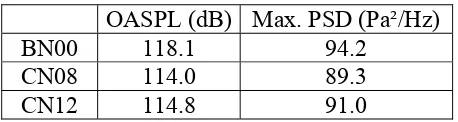
As expected, the use of chevrons has reduced the jet noise at lower frequencies and increased the jet noise at higher frequencies. The maximum sound pressure level and OASPL reduction for each chevron is summarized in table 2.

Table 2. Probe Noise for the Three Nozzles.

OASPL (dB) Max. PSD (Pa²/Hz)

BN00 118.1 94.2

CN08 114.0 89.3

CN12 114.8 91.0

Bridges and Brown (2004) have concluded that the number chevron’s lobes affects directly on the low frequency noise attenuation. Varying the chevron count is a way to reach the target low frequency reduction, without strong high frequency penalty. This fact is confirmed by the RFG simulations. Figure 10 shows that varying the number of chevron lobes from 12 to 8 produces a significant low frequency noise reduction, whilst the high frequency spectrum region is almost unaffected. The maximum value of power spectrum density is decreased and the peak frequency is shifted to lower bands. The apparent reason for this rely on the high noise source volume near the nozzle exit and in the small structures formed near the smaller lobes of the CN12 configuration. For these simulations, the chevron with 8 lobes showed the best noise reduction of 4.1 dB OASPL and a reduction in the peak power spectrum density of 4.9 Pa²/Hz. The high frequency noise is slightly bigger for the CH08, compared with CH12. Hence, there must be an optimal chevron design, concerning the number of lobes, which has to be studied in each specific application, considering the trade-off between high frequency increase and low frequency decrease.

4 Conclusions

behavior of these noise suppression devices was captured by this stochastic model. The magnitude of the noise reductions are also in agreement with the data found in literature (Bridges and Brown, 2004). The effect of the number of chevron lobes also has been evaluated. Bridges and Brown (2004) have concluded that the number chevron’s lobes affects directly on the low frequency noise attenuation, and this fact was confirmed by the RFG simulations. The total noise radiated by a nozzle configuration depends on the turbulent volume and the level of the k within this volume. The model CN12 presented a higher peak PSD and a shifted spectrum shape in the direction of the higher frequencies. This is probably due to high noise source volume near the nozzle exit and the small structures near the smaller lobes of the CN12 configuration. The overall reduction of the CN08 was greater than the CN12, but with a slightly bigger penalty in the high frequency noise.

Future works may use different chevron nozzles to verify the influence of penetration and lobe length in the dynamic and acoustic response. Also, more probes would furnish better insight about the directivity of the chevron noise reduction. The simulations of hot jets, coaxial or supersonic jets are also great challenges today and are of main importance for the aerospace industry.

5 Acknowledgements

The authors thank Embraer and Metacomp for the support given during the development of this work.

References

Andersson, N., Eriksson, L. E., Davidson, L., 2005, “Investigation of an isothermal Mach 0.75 jet and its radiated sound using large-eddy simulation and Kirchhoff surface integration”. International Journal of Heat and Fluid Flow, 26, pp. 393-410.

Batten, P., Ribaldone, E., Casella, M., Chakravarthy, S., 2004, “Towards a Generalized Non-Linear Acoustics Solver”, AIAA paper 2004-3001.

Birch, S. F., 2006, “Noise prediction for Chevron Nozzle Flows”, AIAA Paper 2006-2600.

Bridges, J. Brown, C. A., 2004, “Parametric Testing of Chevrons on Single Flow Hot Jets”, AIAA paper 2004-2824.

Callender, B., Gutmark, E., “Far-Field Acoustic Investigation into Chevron Nozzle Mechanisms and Trends”, AIAA Journal, Vol. 43, No1, 2005, pp. 87-95.

Colonius, T., Lele, S. K., 2004, “Computational aeroacoustics: progress on nonlinear problems of sound generation”, Progress in Aerospace Sciences, 40, pp. 345-416.

Freund, J. B., 2001, “Noise sources in a low-Reynolds-number turbulent jet at Mach 0.9”, J. Fluid Mech., 438, pp. 277-305.

Kenzakowski, D. C., Kannepalli, C., 2005, “Jet Simulation for Noise Prediction Using Advanced Turbulence Modeling”. AIAA paper 2005-3086

Lighthill, M. J., 1952, “On sound Generated Aerodynamically, I. General Theory”, Proc. Roy. Soc., Vo. 216, pp.564-587.

Page, G. J., McGuirk, J. J., Hossain, M., Hughes, N. J., 2002, “A computational and experimental investigation of serrated coaxial nozzles”, AIAA paper 2002-2554.

SAE, 1994, “Gas Turbine Exhaust Noise Prediction”, Aerospace Recommended Practice ARP-876D. Silva, C. R. I. da, Almeida, O. de, 2007, “Investigation of an Axi-symmetric Subsonic Turbulent Jet

using Computational Aeroacoustics tools”. AIAA paper 2007-3656.

Smirnov, A., Shi, S., Celik, I., (2001), “Random Flow Generation Technique for Large Eddy Simulations and Particle-Dynamics Modelling”, ASME J. of Fluids Engineering, 123:359-371. Viswanathan, K., “Does a Model-Scale Nozzle Emit the Same Jet Noise as a Jet Engine?”, AIAA