Development, optimization, and integration of molecular fitting tools and models in UCSF Chimera

Texto completo

(1)Development, optimization, and integration of molecular fitting tools and models in UCSF Chimera Desarrollo, optimización e integración de herramientas y modelos de ajuste molecular en Chimera. Pablo Solar Rodríguez Universitary Master’s Degree in BioInformatics and BioStatistics BioInformatics – Structural and Computational Biology Brian Jiménez García Pablo Chacón – José Ramón López Blanco. 24th May 2017.

(2) LICENCIA (LICENSE). GNU Free Documentation License (GNU FDL) Copyright © 2017 PABLO SOLAR RODRÍGUEZ. Permission is granted to copy, distribute and/or modify this document under the terms of the GNU Free Documentation License, Version 1.3 or any later version published by the Free Software Foundation; with no Invariant Sections, no Front-Cover Texts, and no Back-Cover Texts. A copy of the license is included in the section entitled "GNU Free Documentation License"..

(3) FINAL WORK SHEET. Título del trabajo:. Development, optimization and integration of molecular fitting tools and models in Chimera. Nombre del autor: Pablo Solar Rodríguez Nombre del consultor/a: Brian Jiménez García Nombre del PRA: M. Jesús Marco Galindo Fecha de entrega (mm/aaaa): 05/2017 Titulación:: Área del Trabajo Final:. Máster Universtario BioEstadística. en. BioInformática. y. BioInformática – Biología Computacional y Estructural. Idioma del trabajo: Inglés Palabras clave. Chimera, fitting, computational biology, structural biology, plugin, ADP_EM, iMODFIT. Resumen del Trabajo (máximo 250 palabras): Con la finalidad, contexto de aplicación, metodología, resultados i conclusiones del trabajo. El TFM se encuadra en el campo de la bioinformática estructural y se centra en el desarrollo de herramientas computacionales para interpretar información 3D de proteínas y ácidos nucleicos proveniente de distintas fuentes experimentales como son la crio-microscopía electrónica (EM) y la cristalografía de rayos X. El ajuste macromolecular o fitting es la forma estándar de interpretar la información contenida en un mapa de crio-microscopía electrónica de una determinada macromolécula con las estructuras atómicas disponibles de sus componentes. Se trata de un complicado puzzle donde se encajan estructuras a resolución atómica dentro de un mapa de densidad electrónica a menor resolución. Aunque existen diversas aproximaciones para llevar a cabo el ajuste molecular, son herramientas en desarrollo que es necesario perfeccionar y adaptar al usuario (López‐Blanco/Chacón 2015). El objetivo general de este TFM es la mejora y adaptación de los métodos de ajuste desarrollados por el grupo receptor del doctor P. Chacón, así como su integración dentro del programa UCSF Chimera a través de la realización de unos plugins. Concretamente, las herramientas ADP_EM, Situs e iMODFIT. Al final, se obtendrán una serie de plugins para Chimera desarrollados en Python para las diferentes herramientas y métodos de ajuste molecular desarrollados por el grupo, que se harán públicos a la comunidad científica..

(4) Abstract (in English, 250 words or less): This project lies within the field of structural biology and will be focused on computational tools development to integrate 3D information of proteins and nucleic acids from different experimental sources such as cryo-electron microscopy (EM) or Xray crystallography. Fitting is the standard way of interpreting the information contained in cryo-electronmicroscopy maps of macromolecular structures by means of the available atomic structural components. Multiresolution fitting is a complicated jigsaw puzzle in which the low-resolution 3D EM density map of a macromolecule complex acts as a fuzzy frame to guide the assemblage of interlocking atomic-resolution pieces. Although there are several approaches to perform fitting, those are tools in development phase that needs to be improved and better adapted to the users (López-Blanco, J. R. and Chacón, P. (2015)). The main objective of this project is the improvement and adaptation of these fitting tools developed by P. Chacón’s team, as well as its integration in UCSF Chimera program. Specifically, ADP_EM, Situs e iMODFIT tools. At last, some Chimera plugins will be obtained based on the different fitting tools and models developed by the group..

(5) Index 1. Overview ......................................................................................................... 1 1.1 Project Context and Justification .................................................................... 1 1.2 Project Objectives......................................................................................... 2 1.2.1 General Objectives.............................................................................. 2 1.2.2 Specific Objectives .............................................................................. 3 1.3 Approach and Methods ................................................................................. 4 1.3.1 Software and Technology .................................................................... 4 1.3.2 Hardware .......................................................................................... 7 1.4 Project Planning ........................................................................................... 8 1.4.1 Initial Tasks........................................................................................ 8 1.4.2 Final Tasks ......................................................................................... 9 1.4.3 Initial Tasks Timing ........................................................................... 10 1.4.4 Final Tasks Timing ............................................................................ 11 1.4.5 Project Calendar Comparison ............................................................. 12 1.4.6 Project Milestones ............................................................................ 13 1.4.7 Risk Analysis .................................................................................... 14 1.5 Brief Summary of the Products Obtained ...................................................... 15 1.6 Short description of memory chapters .......................................................... 18 2. Macromolecular Fitting Tools .......................................................................... 20 2.1 Macromolecular Fitting ............................................................................... 20 2.1.1 Rigid Fitting ..................................................................................... 21 2.1.2 Flexible Fitting.................................................................................. 23 2.2 ADP_EM Rigid Fitting Tool ........................................................................... 24 2.3 iMODFIT Flexible Fitting Tool ....................................................................... 29 3. Results ........................................................................................................... 36.

(6) 3.1 Chimera ..................................................................................................... 36 3.2 ADP_EM Plugin for Chimera ........................................................................ 37 3.3 iMODFIT Plugin for Chimera ........................................................................ 47 3.4 Plugins Testing ........................................................................................... 56 3.5 Dissemination of the Plugins ........................................................................ 61 3.6 Conclusions ................................................................................................ 63 3.7 Acknowledgements .................................................................................... 65 4. Glossary ......................................................................................................... 66 5. Bibliography ................................................................................................... 67 6. Appendants .................................................................................................... 69 6.1 ADP_EM Relevant Code .............................................................................. 69 6.2 iMODFIT Relevant Code .............................................................................. 77.

(7) List of Figures Figure 1: Initial Project Calendar. .......................................................................... 12 Figure 2: Final Project Calendar. ........................................................................... 12 Figure 3: Rigid and flexible macromolecular fitting. ................................................ 20 Figure 4: 6-Dimensional direct search. .................................................................. 22 Figure 5: Normal vibration modes......................................................................... 23 Figure 6: Radial and spherical sampling. ................................................................ 27 Figure 7: Modelling the atomic structure using ADP_EM. ........................................ 27 Figure 8: ADP_EM Workflow. ............................................................................... 28 Figure 9: iMODFIT Workflow. ............................................................................... 32 Figure 10: Flexible fitting of the thermosome into an experimental EM map at 10Å.. 33 Figure 11: Flexible fitting of the GroEL into an experimental EM map at 10 Å ............ 34 Figure 12: Flexible fitting of the RepB in the presence of DNA using iMODFIT............ 35 Figure 13: A snapshot of the UCSF Chimera program. ............................................. 36 Figure 14: ADP_EM entry menu in Chimera. .......................................................... 38 Figure 15: ADP_EM basic GUI in Chimera............................................................... 38 Figure 16: ADP_EM GUI status just before perform fitting ....................................... 40 Figure 17: ADP_EM fitting process shown by the log window. ................................. 41 Figure 18: ADP_EM expert GUI in Chimera. ........................................................... 42 Figure 19: ADP_EM process finished. .................................................................... 42 Figure 20: ADP_EM Results panel with all the calculated solutions dropped down..... 43 Figure 21: ADP_EM Solution 1 fitted into the map. ................................................. 44 Figure 22: ADP_EM Solution 8 fitted into the map. ................................................. 44 Figure 23: ADP_EM Solution 10 fitted into the map. ............................................... 45 Figure 24: Copies of solutions 1, 8 and 10 and molecule positioned in solution 17. .... 45 Figure 25: A snapshot of the user guide. ................................................................ 46.

(8) Figure 26: Objects loaded (A) and objects moved (B). ............................................. 46 Figure 27: Solution 16 of the moved molecule from Figure 25b. .............................. 47 Figure 28: iMODFIT entry menu in Chimera. .......................................................... 48 Figure 29: iMODFIT simplest GUI in Chimera. ......................................................... 48 Figure 30: iMODFIT GUI status just before start fitting. ........................................... 50 Figure 31: iMODFIT fitting process shown by the log window. ................................. 50 Figure 32: iMODFIT expert GUI in Chimera. ........................................................... 51 Figure 33: iMODFIT process finished. .................................................................... 51 Figure 34: iMODFIT Results panel. ........................................................................ 52 Figure 35: iMODFIT showing the original molecule. ................................................ 53 Figure 36: iMODFIT showing the fitted molecule. ................................................... 53 Figure 37: iMODFIT showing the fitted molecule and its copy in the Model Panel...... 54 Figure 38: iMODFIT showing the original molecule and the fitted copy. .................... 54 Figure 39: Frame 9 of the trajectory movie generated by iMODFIT. ......................... 55 Figure 40: Frame 1 of the trajectory movie generated by iMODFIT. ......................... 55 Figure 41: A snapshot of the user guide................................................................. 56 Figure 42: Snapshot of the ADP_EM Chimera plugin the receiving group web. .......... 62 Figure 43: : Snapshot of the iMODFIT Chimera plugin the receiving group web. ........ 63.

(9) 1. Overview 1.1 Project Context and Justification Advances in current biology and medicine depend on understanding the actions and interactions of large molecular complexes. The characterization of these macromolecules can only be approached with the coordinated application of different complementary experimental techniques. The hybrid methods allow combining computationally and in an automatic and reproducible way the structural information provided by the experimental techniques. It is a challenge in how computational methods would assist on characterizing, at atomic level of the different functional states of the macromolecules in solution and, therefore, to understand the molecular mechanisms of the main actors of the different biological functions. In this context, one of the most interesting and fruitful fields of current structural bioinformatics focuses on the development of different methodologies for integrating structural information into different resolutions. The relevance and timeliness of this field has aroused my interest. I think it is an ideal framework to apply the knowledge acquired in the Master and it will guide my professional training towards the field of research in one of the most powerful research groups of this area at national and international level, like Pablo Chacón’s group. Thus, according to everything described above, this project lies within the field of structural biology and will be focused on computational tools development to integrate 3D information of proteins and nucleic acids from different experimental sources such as cryo-electron microscopy or X-ray crystallography. Fitting is the standard way of interpreting the information contained in electron-microscopy (EM) maps of macromolecular. 1 2.

(10) structures by means of the available atomic structural components. Multiresolution fitting is a complicated jigsaw puzzle in which the low-resolution 3D EM density map of a macromolecule complex acts as a fuzzy frame to guide the assemblage of interlocking atomic-resolution pieces. Although there are several tools to perform fitting, they are in development phase that need to be improved and better adapted to the users (López-Blanco, J. R. and Chacón, P. (2015)). The main objective of this project is the improvement and adaptation of these fitting tools developed by P. Chacón’s receiving group, as well as its integration in UCSF Chimera program. Specifically, ADP_EM, Situs and iMODFIT tools. At last, some Chimera plugins will be obtained based on the different fitting tools and models developed by the group and published to the scientific community (dissemination).. 1.2 Project Objectives 1.2.1 General Objectives Two main objectives will be defined in this project: training objective and fitting tools development objective. This section describes the objectives from a global and conceptual perspective. The training objective will serve to get familiarized with the computational techniques of structural integration, specifically the fitting methods developed by the receiving team. Once the brief training period has been completed, the main and most important objective would be the development, improvement, and adaptation of the molecular fitting methods developed by the receiving group (Lopéz-Blanco, J. R. and P. Chacón (2013), Chacón, P. and W. Wriggers (2002), Garzón, J. I., J. Kovacs, R. Abagyan and P. Chacón (2007)), like ADP_EM, iMODFIT, or Situs. 2.

(11) 1.2.2 Specific Objectives Training Objectives 1. Familiarization with theory and software of molecular fitting tools developed by the group, particularly with packages: • Situs (http://situs.biomachina.org) • ADP_EM (http://chaconlab.org/methods/fitting/adpem) • iMODFIT (http://chaconlab.org/methods/fitting/imodfit ) 2. Familiarization with other bioinformatics fitting approaches like: • mdff (http://www.ks.uiuc.edu/Research/mdff/) • gEMfitter (http://gem.loria.fr/gEMfitter/) • Integrative Modeling (https://integrativemodeling.org/ ) • Rosseta (https://www.rosettacommons.org/) Development Objectives 1. Development, improvement, optimization, and the integration of ADP_EM, iMODFIT, and Situs into UCSF Chimera. It is intended to improve de efficiency and usability of these tools trough code improvements (C and C++) and, specifically, develop Chimera plugins in Python for Chimera program, which is the most used visualization tool in the field of electron microscopy. o ADP_EM is a priority while iMODFIT and Situs plugins would be implemented as long as the project’s timing and needs allow.. 3.

(12) 2. Depending on the project’s timeline progress, integration of other molecular fitting programs such as geMfitter and COLORES (Situs) will be explored. 3. At last, the obtained Chimera plugins will be properly released to the scientific community.. 1.3 Approach and Methods The field of application is such a specific field that requires prior training. For this reason, in a first stage a strategy has been combined into a brief training to understand and get familiar with the problem of molecular fitting with the introduction to the approaches used in the field. This stage will also be useful to identify which tools could be improved and the way to do it. In the second stage, the fitting tools will be developed and improved through computational knowledge based in C/C++ and Python. The technologies, software, and hardware required and used to perform both stages will be detailed in the following sections.. 1.3.1 Software and Technology •. Products and plugins will be developed in Python mostly which is the base programming language where Chimera is built. Python version will be the latest and updated version supported by the development computers and frameworks. Syntactic analysis will be used to ensure the quality of the code created.. • It may be necessary the use of C and C++ to create shared libraries and pipes that allow a bidirectional communication between Chimera plugins and the fitting processes like. 4.

(13) ADP_EM or iMODFIT. This point is open due to variations in development requirements. • C and C++ compilers that will be used for the fitting tools processes will be Intel Parallel Studio XE which offers, apart from speed and management compilation, some useful APIs like Fourier transforms that are necessary in this project, as it will be seen in later chapters. • Changes and versions of products during the development phase will be handled through Git repository in the internal intranet that the receiving group is actually using for their works. • Chimera plugins development, the main objective of this project, use Python in order to be dynamically used by users. This is, that one user can load a plugin in Chimera from any folder location, i.e. independently of the administrative permissions. • All products obtained will a simple, friendly user guide with detailed installation instructions. • All products obtained will be published to the public trough the official media of the receiving group. In addition, they will be deployed in an online repository like GitHub so that they are use as much as possible. o It is also intended to contact the official developers of Chimera to include the products natively in the program, if they consider them fit and robust enough. • In the first stage of development, plugins will be coded for Linux and Mac OS X, trying to adapt them to Windows platforms too, but this will depend on project deadlines, requirements and changes. • Plugins developed should be compatible with previous and future versions of Chimera, as long as Chimera standards do not change.. 5.

(14) •. Since the plugins will handle several atomic structures in form of PDBs and EM density maps of biological macromolecules, a developed code quality will be necessary to ensure a good flow and memory management, as well as the own session of Chimera. It will also be necessary to take care of the computational cost and the complexity of the code developed in the products.. • A priori it is not possible to establish a usual testing strategy for the plugins developed since it is necessary to restart Chimera every time modifications are to check them. Thus, two phases of testing can be established: o Development phase testing: basic and simple tests about the correct functionality of different requirements that are demanded to the plugins. o Post-development phase testing: overload and stress. testing with real data that will check the performance of the plugins in professional tasks. •. Products and plugins obtained should be developed with quality enough to be improved in a future with new functionalities in a simple, fast, secure and robust way.. •. Support and development will be in constant supervision and change.. 6.

(15) 1.3.2 Hardware This project will be carried out in a MacBook Pro 15” with the following characteristics:. Processor. Memory. CPU speed: 2.3 GHz. Installed RAM: 8 GB (2x4GB). CPU Type:. Quad Core i7. Max. Amount: 8.0 GB. Cores:. 4. Nr. of Slots:. 2. RAM Speed:. 1600 MHz. RAM Type:. DDR3, SDRAM. Bus Speed: 5 GT/s DMI Cache:. 6 MB L3 cache. 64-bit:. Yes. Turbo Boost: Up to 3.3 GHz. Storage and Media. Graphics. Hard Drive: 500 GB, 5400 rpm.. Display Size:. 15.4-inch. Drive Brand: Hitachi or Toshiba. Graphics Card:. NVIDIA GeForce GT 650M Intel HD Graphics 4000 1 GB (GT650). Drive Bus:. Serial-ATA. Card Memory:. Optical Drive: This unit has an 8x SuperDrive built in. Optical Bus: Serial-ATA. Max. Resolution: 1440 x 900 BLU / Coating:. LED TFT, Glossy.. Other Media: -. Networking. Operating System and Software. AirPort:. Original OS:. Built-in Airport Extreme (802.11 a/b/g/n).. 10.7.4 Lion. Ethernet: 10/100/1000BASE-T (RJ-45). Maximum OS: Latest release of Mac OS X. Bluetooth:Built-in Bluetooth 4.0. Minimum OS: OS X 10.7.3 Build 11D2097. Infrared: For use with Apple Remote only. Modem: None. 7.

(16) 1.4 Project Planning The planning has been subject to changes that were a consequence of variations or modifications suffered by the different products that were developed, either by internal or external requirements. In this section, tasks and its deadlines variations, calendars, Gantt charts and project milestones will be exposed.. 1.4.1 Initial Tasks 1. Training with molecular fitting theory and software developed by the receiving group: a. Situs. . 2. days. b. ADP_EM. . 14. days. c. iMODFIT. . 3. days. 2. Familiarization with other bioinformatics fitting approaches: a. gEMfitter. . 1. day. b. mdff. . 1. day. c. Integrative Model. . 1. day. d. Rosetta. . 1. day. 3. Improvement and adaptation of ADP_EM and iMODFIT. Chimera plugins development: a. Chimera plugins definition. . 4. days. b. ADP_EM Chimera plugin GUI. . 5. days. c. ADP_EM fitting process in Chimera . 8. days. . 6. days. d. ADP_EM plugin tests and results. 4. Development of other approaches like iMODTFIT or Situs: 8.

(17) a. Subject to availability and changes. . 10. days. i. if it not possible, ADP_EM plugin will be perfected 5. Project Memory creation and presentation . 10. days. a. Project Memory creation. . 7. days. b. Project presentation. . 5. days. 1.4.2 Final Tasks 1. Training with molecular fitting theory and software developed by the receiving group: a. Situs. . 1. day. b. ADP_EM. . 17. days. c. iMODFIT. . 3. days. 2. Familiarization with other bioinformatics fitting approaches: a. gEMfitter. . 0,5. day. b. mdff. . 0,5. day. c. Integrative Model. . 0,5. day. d. Rosetta. . 0,5. day. 3. Improvement and adaptation of ADP_EM and iMODFIT. Chimera plugins development: a. Chimera plugins definition. . 4. days. b. ADP_EM Chimera plugin GUI. . 8. days. 12. days. 9. days. c. ADP_EM fitting process in Chimera  d. ADP_EM plugin tests and results 9. .

(18) 4. Development of other approaches like iMODTFIT or Situs and project memory and presentation: a. Subject to availability and changes. . 10. days. i. if it not possible, ADP_EM plugin will be perfected ii. Project Memory creation. . 7. days. iii. Project presentation. . 5. days. 1.4.3 Initial Tasks Timing Stage. Task Step. 1. Training 2. Chimera Development. a. 2. b. 14. c. 3. a. 1. b. 1. c. 1. d. 1. a. 4. b. 5. c. 8. d. 6. -. 10. a. 7. b. 5. 3. 4 Memory and Presentation. Step Days. 5. Task Days. Stage Days. 19. 23 4. 66. 23. 10. Total Days. 33. 10 10. 10.

(19) 1.4.4 Final Tasks Timing Stage. Task Step. 1. Training 2. Step Days. a. 1. b. 17. c. 3. a. 0,5. b. 0,5. c. 0,5. d. 0,5. a. 4. b. 8. c. 12. d. 9. a. 10. Task Days. Stage Days. Total Days. 21. 23 2. 66. Chimera Development. Other approaches, Memory and Presentation. 3. 4. 11. 33. 33. 10. 10.

(20) 1.4.5 Project Calendar Comparison. Figure 1: Initial Project Calendar.. Figure 2: Final Project Calendar.. 12.

(21) 1.4.6 Project Milestones Project Starting. 22.02.2017. Training Stage Starting. 22.02.2017. Situs. 22.02.2017-22.02.2017. iMODFIT. 23.02.2017-27.02.2017. UOC PEC1 Starting. 01.03.2017. ADP_EM. 28.02.2017-22.03.2017. UOC PEC2 Ending. 15.03.2016. Other approaches. 23.03.2017-24.03.2017. Training Stage Ending. 24.03.2017. UOC PEC2 Starting. 16.03.2017. Chimera Development Stage Starting. 27.03.2017. Chimera plugins definition. 27.03.2017-30.03.2017. ADP_EM Chimera plugin GUI. 31.03.2017-11.04.2017. UOC PEC2 Ending. 05.04.2017. UOC PEC3 Starting. 06.04.2017. ADP_EM fitting process in Chimera. 12.04.2017-27.04.2017. ADP_EM plugin tests and results. 28.04.2017-10.05.2017. Chimera Development Stage Ending. 10.05.2017. UOC PEC3 Ending. 10.05.2017. Others, Memory and Presentation Stage Starting. 11.05.2017. UOC PEC4 Starting. 11.05.2017. Other approaches. 11.05.2017-24.05.2017. 13.

(22) Memory. 11.05.2017-19.05.2017. Presentation. 18.05.2017-24.05.2017. Others, Memory and Presentation Stage Ending. 24.05.2017. UOC PEC4 Ending. 24.05.2017. 1.4.7 Risk Analysis During the development phase, some risks had to be taken into account that could have affected the achievement of the project and its final outcome: • Changes/modifications of the theoretical approaches of the processes involved: methods, fittings, etc. E.g., introducing a new set of theoretical basis into the fitting methods that were initially not taken into account. • Changes/modifications of the practical approaches of the processes involved. E.g., introducing new GUI functionalities in the ADP_EM plugin that were initially not taken into account. • Changes/modifications in the different tools used during the development of the project. E.g., a new version of Chimera that might have caused compatibility issues and forced to redo some parts of the project. • Computational limitations of the different used resources. E.g., different tests during the testing phase might have had a high computational cost and caused a delay this stage. • Limitations of Chimera that have entailed a rethinking and/or delay before not foreseen. For example, modifications made to different plugins required restarting Chimera every time to check them. This affected directly to the development stage. 14.

(23) Therefore, it is reiterated that the project, and specifically during its development phase, was subject to all kinds of changes, both practical and theoretical, that were resolved as progress was made in the achievement of the different products.. 1.5 Brief Summary of the Products Obtained Training Stage • In-depth level knowledge, theoretical and practical, as well as different application situations of the ADP_EM molecular fitting model. • Medium level knowledge and practical application of the iMODFIT molecular fitting model. • General knowledge and practical application of the Situs molecular fitting model. • Basic knowledge and practical application of the gEMfitter molecular fitting model. • Basic knowledge and practical application of the mdff molecular fitting model. • Basic knowledge and practical application of the Rosetta molecular fitting model. Development Stage • A complete dummy Chimera plugin without any kind of functionality, developed in Python, which can be loaded and integrated in Chimera. In addition, this product can be used as a template to create new plugins in Chimera.. 15.

(24) • A complete Chimera plugin for the ADP_EM molecular fitting model and process with the following functionalities: o Ability to host the plugin in any user folder and allow its loading inside Chimera dynamically, regardless of the chosen directory. ▪ The plugin consists of a directory with the necessary Python files to be loaded in Chimera through a native loading dialog. ▪ An executable C-version of ADP_EM to run the process inside the plugin in Chimera. o Ability to load density maps and atomic structures from any location, allowing independent operation of the plugin and not forcing the user to have to host these resources within the plugin directory. o Graphic User Interface (GUI) with all the options needed to execute the ADP_EM process. ▪ This GUI is capable of interacting with other native modules and plugins already existing in Chimera, such as the Volume Viewer module that is related with density maps. o Validation of all the inputs introduced by the user in the GUI. o Calling to ADP_EM with all the inputs validated to perform exhaustive fitting calculations. o Generation of all the fitting solutions from the ADP_EM binary output (6-dimensions = 3 rotational + 3 translational for each solution). o Visualization of the different solutions in Chimera, directly accessible from the plugin's own GUI. In addition, the user. 16.

(25) can interact with the solutions and save them for later analysis. • An executable C version of the ADP_EM molecular fitting tool optimized and adapted to be used in Chimera. This version is included inside the own directory of the plugin. o Any changes that have to be made in the Chimera plugin will not affect the fitting tool itself and vice versa, any modifications that have to be made to the ADP_EM process will not affect the plugin. o This ADP_EM version is capable of communicating bidirectionally with Chimera in real time effectively. • A complete Chimera plugin for the iMODFIT molecular fitting model and process. o Ability to host the plugin in any user folder and allow its loading inside Chimera dynamically, regardless of the chosen directory. ▪ The plugin consists of a directory with the necessary Python files to be loaded in Chimera through a native loading dialog. ▪ An executable C-version of iMODFIT to run the process inside the plugin in Chimera. o Ability to load density maps EM and atomic structures from any location, allowing independent operation of the plugin and not forcing the user to have to host these resources within the plugin directory. o Graphic User Interface (GUI) with all the options needed to execute the iMODFIT process. ▪ This GUI is capable of interacting with other native modules and plugins already existing in Chimera,. 17.

(26) such as the Volume Viewer module that is related with maps of density or MD Movie. o Validation of all the inputs introduced by the user in the GUI. o Calling to iMODFIT with all the inputs validated to perform exhaustive fitting calculations. o Generation of all the fitting solutions from the iMODFIT process raw files. o Visualization of the different solutions in Chimera, directly accessible from the plugin's own GUI. In addition, the user can interact with the solutions and save them for later analysis. • An executable C version of the iMODFIT molecular fitting tool, optimized and adapted to be used in Chimera. This version is included inside the own directory of the plugin. o Any changes that have to be made in the Chimera plugin will not affect the fitting tool itself and vice versa, any modifications that have to be made to the iMODFIT process will not affect the plugin. o This iMODFIT version is capable of communicating bidirectionally with Chimera in real time effectively.. 1.6 Short description of memory chapters Below are described the theoretical and practical chapters related to this work, which will be further detailed in later sections:. 18.

(27) • Macromolecular Fitting: this chapter puts the molecular fitting into context, why it is used, and what major experimental techniques exist. o Rigid Fitting: it explains the rigid fitting method, why and when it is used, what the underlying idea is, and what mathematical theories it applies (such as Fast Rotational Matching [FRM]) and introduces ADP_EM. o Flexible Fitting: it explains the flexible fitting method, why and when it is used, what the underlying idea is, what techniques it applies (such as Normal Mode Analysis [NMA]) and introduces iMODFIT. • ADP_EM Rigid Fitting Tool: this chapter introduces the ADP_EM method with the mathematical theory on which it is based. In particular, it explains how the search space is rotationally accelerated using Fast Rotational Matching (FRM) with spherical harmonics along with a small example. In addition, it outlines the process workflow scheme. • iMODFIT Flexible Fitting Tool: it details the iMODFIT method and the mathematical theory on which it is based. It explains how the Normal Mode Analysis (NMA) in Internal Coordinates (IC) is used and how the different graining models are applied. In addition, it outlines the process workflow scheme. Finally, the Results section is presented, which details the plugins developed for the methods presented in these chapters along with all the associated features.. 19.

(28) 2. Macromolecular Fitting Tools 2.1 Macromolecular Fitting Density maps obtained by electron microscopy can be interpreted using available atomic structures. By fitting these structures inside low/medium resolution maps it is possible to obtain quasi-atomic information in order to unravel the functioning of macromolecular complexes (Wriggers, W. and Chacon, P. (2001)). When available atomic structures and maps are in the same conformation, it is enough to find the correct orientation between them using a rigid fitting strategy. However, in multiple cases the conformations observed in maps are significantly different from those ones that are in crystals. In these situations, it is necessary to employ a flexible fitting strategy to take into account the different conformations.. Rigid. Flexible Figure 3: Rigid and flexible macromolecular fitting. When the density map (left) and the atomic structure (above) have roughly the same conformation as the target map (right), the fit must be rigid. If the available atomic structure has a different conformation (below) to that of the target map, the setting must be flexible.. 20.

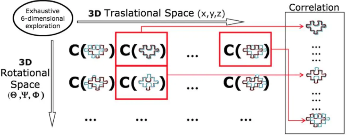
(29) In this project, two macromolecular fittings are presented. The first one is rigid-based, ADP_EM, and the second one is flexible-based, iMODFIT.. 2.1.1 Rigid Fitting A number of high performance fitting programs have been developed over the last year to rigidly adjust atomic structures within density maps when the conformations of both are similar. To do this, there are several programs to carry out this task: SITUS (Wriggers, W., Milligan, R.A. y McCammon, J.A. (1999)), EMFIT (Rossmann, M.G. (2000)), DOCKEM (Roseman, A.M. (2000)), FOLDHUNTER (Jiang, W., Baker, M.L., Ludtke, S.J. y Chiu, W. (2001)), COLORES (Chacón, P. and W. Wriggers (2002)), COAN (Volkmann, N. y Hanein, D. (2003)), 3SOM (Ceulemans, H. y Russell, R.B. (2004)) and ADP_EM (Garzon, J.I., Kovacs, J., Abagyan, R. y Chacon, P. (2007a)). In general, these tools perform an automated search of the all possible relative rotations and translations to maximize a scoring function. This score, typically a score correlation function, is calculated between the target experimental EM map and a simulated probe map of the atomic structure (Wriggers, W. and Chacon, P. (2001), Fabiola, F., Chapman, M.S. (2005)). Despite its successful application, the exhaustive search performed by the majority of these docking tools is a very time-consuming process, and therefore they are not ready to support highthroughput fitting process. In this context, the set of possible positions between objects forms a vast search space. In the case of fitting only two objects, it is necessary to explore a 6-Dimensional space composed of a 3D translational space (spatial position of one object with respect to another defined by three Cartesian values) and a 3D rotational space (rotation of an object with respect to the another defined by three angular values). The simplest approach to this exploration (Figure 4), consisting of a systematic sampling of 6Dimensional space, is impracticable if relatively small search intervals are used. Assuming a rigid fitting in which the rotational interval of 6°, for each translation it will be necessary to explore more than 105 rotations. If the maps also have dimensions of 21.

(30) 100x100x100 cells or voxels, then the number of possible translations can be 106 (the center of one of the maps is superimposed on each voxel of the other). In summary, systematic sampling in this case may require the exploration of approximately one hundred billions of map positions relative to the other, with the consequent computational cost.. Figure 4: 6-Dimensional direct search. The 6-Dimensional search discreetly explores the maximum number of possible positions and orientations of an object with respect to another. For each of these combinations the correlation between the two objects is calculated. In a final step, the possible solutions are ordered according to the correlation.. To increase efficiency, some methodologies have been developed to accelerate the search for some of the degrees of freedom that make up their space. The classical approach used to accelerate this search is to calculate the correlation in the frequency space. Through the combined use of the convolution theorem and Fast Fourier Transform (FFT) calculation techniques it is possible to accelerate the search in the translational space, requiring only a systematic exploration of the rotational space. Thus, for each rotation, the correlation in the translation space is calculated by: (1) Where 𝑀𝜆𝐴 and 𝑀𝜆𝐵 are the electron density matrices representing three-dimensional maps. This type of fitting, called Fast Translational Matching (FTM) (Katchalski-Katzir, E., Shariv, I., Eisenstein, M., Friesem, A.A., Aflalo, C., and Vakser, I.A. (1992)), has already been successfully used in bioinformatics applications (Wriggers, W. and Chacon, P. (2001), (Eisenstein, M. and Katchalski-. 22.

(31) Katzir, E. (2004)). Alternatively, it is also possible to accelerate the rotational space search by combining a suitable representation of the rotational space and the use of spherical harmonics (Ritchie, D.W. and Kemp, G.J. (2000), Kovacs, J.A. and Wriggers, W. (2002)). This methodology, called Fast Rotational Matching (FRM), allows obtaining a search that is better adapted, and therefore faster, to the nature of the bioinformatics fittings described below. The ADP_EM algorithm combines FTM and FRM while Situs only uses FFT. The first one is described in later chapters.. 2.1.2 Flexible Fitting Flexible fitting methods are used to consider the conformational differences between the atomic structures and the density maps. Although the most commonly used method to study the flexibility of macromolecules are those based on Molecular Dynamics (MD) and NMA (Normal Mode Analysis), other alternative approaches have also been used successfully. The following section briefly discuss the NMA method in which flexible fitting tool used in this work is based (iMODFIT). One of the most interesting alternatives to MD for studying the flexibility of macromolecules is the NMA. The NMA is an effective computational method for the study of large-scale and collective macromolecular motions despite its limitations (Kovacs, J.A., Chacon, P., Cong, Y., Metwally, E. and Wriggers, W. (2003)). The NMA can model with relative ease the collective and large amplitude movements of large macromolecular complexes. The main approximation of 23. Figure 5: Normal vibration modes The three lower energy modes of the protein structure of the adenylate kinase (4ake) protein have been shown with arrows..

(32) this methodology is that the potential and kinetic energies vary quadratically around the minimum energy conformation of the system. From this assumption it is possible to decompose the macromolecular motion in a series of modes of deformation. These modes form an orthonormal basis of vectors which describes all possible shifts or deformations around the equilibrium conformation, that is, any movement can be expressed as a linear combination of these modes. The first three modes of the adenylate kinase protein are shown in Figure 5. Each of them is associated with an energy (or frequency) so that it is possible to determine those movements that are more energy-efficient. Note that at higher frequency, higher energy, and vice versa. It is not possible to identify which modes are functionally relevant without additional experimental data. However, in general, they will almost always be one or a few of the lowest frequency because they represent the conformational transitions with lower energy cost. In principle, it is possible to study the function of biomolecules by filtering out the less important, high-frequency motions, and focusing on the most dominant low frequency (lower energy) modes (Ma, J. (2005)).. 2.2 ADP_EM Rigid Fitting Tool ADP_EM is a rigid body fitting method used for interpreting the information contained in EM maps. The atomic structures are located inside the experimental map by maximizing their cross correlation. ADP_EM combines the Fast Rotational Matching method (FRM) (Kovacs, J.A. and Wriggers, W. (2002)) and translational scans using spherical harmonics and a convenient formulation of the three-dimensional rotation. Due to this, it is possible to improve the search efficiency and exhaustiveness of the rotational space.. 24.

(33) The computational solution of the search problem can be reduced to finding the relative orientation and translation which maximizes the density cross-correlation of the structures/maps to be fitted. For a given rotation and translation the cross correlation is defined as the scalar product between the EM experimental map 𝜌𝑙𝑜𝑤 , and a low-pass filtered version of the atomic structure, 𝜌ℎ𝑖𝑔ℎ :. 𝑪(𝑻, 𝑹) = ∫ 𝝆𝒍𝒐𝒘 × 𝛀𝑻 𝚲𝑹 𝝆𝒉𝒊𝒈𝒉. (1). ℝ𝟑. where Ω 𝑇 and Λ𝑅 denote the translational and rotational operators, respectively. To find the highest correlation values, some previous approaches perform a systematic rotational scan of an atomic structure (𝜌ℎ𝑖𝑔ℎ ) relative to a fixed map (𝜌𝑙𝑜𝑤 ), combined with a Fast Fourier Transform (FFT)-accelerated translational search based on the convolution theorem. This well-known exhaustive search protocol is borrowed from the protein-protein docking field (Gabb, H.A., Jackson, R.M. and Sternberg, M.J. (1997), Katchalski-Katzir, E., Shariv, I., Eisenstein, M., Friesem, A.A., Aflalo, C. and Vakser, I.A. (1992), Vakser, I.A., Matar, O.G. and Lam, C.F. (1999)). In contrast, ADP_EM also accelerates the rotational search providing higher efficiency. This method, named Fast Rotational Matching (FRM), uses a spherical harmonics parameterization of the three-dimensional rotation to efficiently compute the correlation of all rotations for each position (Fig.6). A detailed description of the theory underlying the FRM method was given elsewhere (Chacón, P. and W. Wriggers (2002), Kovacs, J.A., Chacon, P., Cong, Y., Metwally, E. and Wriggers, W. (2003). Briefly, density functions to be fitted are first approximated by expansions in a basis of spherical harmonic (SH) functions. To this end, the EM map is partitioned into concentric spherical layers each of which is represented by finite sums as:. 25.

(34) B 1.  low ( r ,  ,  ) . l. C l  0 m  l B 1.  high ( r ,  ,  ) . low ( r )Ylm (  ,  ) lm. (2). l. C l  0 m  l. high ( r )Ylm (  ,  ) lm. where: (𝑟). • 𝐶𝑙𝑚 are coefficients associated with a specific, complexvalued spherical harmonic function 𝑌𝑙𝑚 (𝛽, 𝜆) defined on the unit sphere; • 𝑙 ≥ 0 and – 𝑙 ≤ 𝑚 ≤ 𝑙 are the SH degree and order, and 𝛽 and 𝜆 are the co-latitude and longitude, respectively. • According to the sampling theorem, the number of sampling points (in each 𝛽 and 𝜆) used is equal to twice of the bandwidth B. Instead of recasting the exhaustive search into a formulation involving five angles and just one translational parameter (Kovacs, J.A., Chacon, P., Cong, Y., Metwally, E. and Wriggers, W. (2003)), here the three rotational degrees of freedom are accelerated, while the three translational ones are simply scanned. Considering only the rotational part, the fitting function can now be expressed in terms of an inverse Fourier transform of the SH transforms (eq. 2) of the density maps (Kovacs, J.A. and Wriggers, W. (2002)):.  l C ( R )  FTm , h , m '  d mh  l 1. . l d hm. C 0. low high ( r ) Clm ( r ) lm. 2. r dr.  . (3). 𝑙 where the 𝑑𝑚𝑛 are real coefficients that define the matrix elements of the irreducible representations of the three-dimensional rotation group. This expression can be computed very efficiently by 𝑙 precomputing the coefficients 𝑑𝑚𝑛 and by using as upper limit of integration the maximum shell radius for which the density has nonzero values. In this way, eq. 3 allows, for a given translation, a very fast calculation of the correlation function for all rotations, which. 26.

(35) will be sampled at twice the bandwidth B used in the harmonic transformation of the maps (eq. 2). For example, B=16 corresponds to scanning 16,000 rotations with a sampling step of 11.25°. If the rotational sampling step is set to 5.6° (B=32), more than 130,000 rotations will be explored. Thus, this method offers an efficient and customizable rotational screening (extracted with the permission of the receiving group (Garzón, J. I., J. Kovacs, R. Abagyan and P. Chacón (2007))).. Figure 6: Radial and spherical sampling. The figure on the right represents the radial sampling of the electronic density of the 1lza protein (left). Points with the highest electronic density are shown in red, with lower density in blue. Each spherical layer of this radial sampling is then used to perform the expansion on the basis of spherical harmonics.. The exhaustive search is then performed by applying this FRM rotational scan on a list of translational points that uniformly cover all the search space. Moreover, the translational space is limited to Figure 7: Modelling the atomic structure using ADP_EM. ADP_EM adjusts the atomic structure of the component to the map areas at low resolution where the correlation of electronic densities is greater. In the example shown, since the complex is a trimer (made up of three identical structures) there are three correlation maxima.. 27.

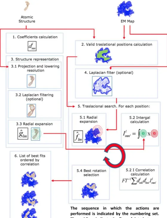
(36) positions on which the dimension of the atomic structure roughly fits inside the experimental EM map to prevent scanning nonsense points. There are other translational strategies, such as radial search (useful for structures with holes) or center-based search (practical for fitting structures with similar dimensions) (Kovacs, J.A., Chacon, P., Cong, Y., Metwally, E. (2003). These sampling schemes take advantage of geometry but their application range is not universal as the uniform sampling scheme using a mask. Therefore, the masking strategy is set as default in this project.. The sequence in which the actions are performed is indicated by the numbering set. The red lines indicate the flow of data between the different actions. Figure 8: ADP_EM Workflow.. 28.

(37) Although the density cross-correlation works reasonably well, in particular cases may lead to ambiguous false positives. This can be critical when the resolutions are low, typically less than 15 Å, and small components are to be placed in a large density map. Some alternatives can be taken into account to improve the fitting contrast. For example, the fitting can be performed by a local correlation criterion (Roseman, A.M. (2000), Rath, B.K., Hegerl, R., Leith, A., Shaikh, T.R., Wagenknecht, T. and Frank, J. (2003)), or the maps can be pre-filtered with a Laplacian kernel (Chacón, P. and W. Wriggers (2002)). Since its implementation does not need any change in the registration scheme, here the fitting is performed with Laplacian-filtered maps instead of the original density maps. The strategy of convolving the maps with a Laplacian kernel improves the numerical contrast among potential solutions, by including both density and contour overlap. A new version of ADP_EM and a plugin were developed and integrated in Chimera. This will be described in later chapters.. 2.3 iMODFIT Flexible Fitting Tool iMODFIT is an approach to obtain a flexible atomic model from a low-resolution experimental map and an initial atomic structure in different conformations. Basically, NMA in IC reduces the conformational search space to physically realistic collective motions and implicitly maintains the covalent structures, thus preventing distortions. Because lowfrequency modes computed in IC provide a reasonable and inexpensive direct view of the relevant conformational space, it is possible to use the most probable deformation directions encoded in this essential space to flex the atomic structure while maximizing the density overlap with the target experimental map. The NMA decomposes motion into a set of collective deformation modes. This reduces dramatically the number of variables and. 29.

(38) improves efficiency (Bray, J.K., Weiss, D.R., Levitt, M., 2011, Kovacs, J.A., Cavasotto, C.N., Abagyan, R., 2005, López-Blanco, J.R., Garzon, J.I., Chacon, P., 2011, Lu, M., Poon, B., Ma, J., 2006, Mendez, R., Bastolla, U., 2010). The iMOD NMA engine is used to compute low-frequency modes in IC (Lopez-Blanco, J.R., Garzon, J.I., Chacon, P., 2011). In NMA, the macromolecule is modelled as a series of pseudo-atoms connected by harmonic springs. The modes are calculated by solving a general eigenvalue problem that diagonalizes the second derivative matrices of potential and kinetic energies (Lopéz-Blanco, J. R. and P. Chacón (2013)):. HU  kTU where U  (u1 , u2 ,..., u N ),. (1). Here, 𝒖𝑘 is the 𝑘 𝑡ℎ deformation vector with its associated 𝜆𝑘 eigenvalue, and Η and Τ are the kinetic energy matrixes, respectively. The equation of the potential energy is (Lopéz-Blanco, J. R. and P. Chacón (2013)): V   Fij (rij  rij0 )  s(  0 ) 2. i j. . 2. . where Fij  1 1  rij0 3.8. 6. . (2). One of the most interesting advantages of iMODFIT is its versatility because it can handle different types of complexes and different graining levels to represent structures: • Heavy-atoms (HA): considers all heavy atoms for proteins and nucleic acids (next-hydrogen). • Five pseudo-atoms (C5): uses NH, Cα, and CO, including a Cβ and virtual mass located at the mass center. • Cα: select a single Cα atom per amino acid for proteins. Indeed, these different representations had to be handled in the Chimera plugin developed that will be seen in later chapters. iMODFIT workflow is summarized in the Figure 9. In essence, the tool interactively explores the lowest frequency modes to improve 30.

(39) the cross correlation with a target map. The atomic structure must be approximately placed in the correct position inside the map. To this end, ADP_EM (Garzón, J. I., J. Kovacs, R. Abagyan and P. Chacón (2007)) or COLORES (Chacón, P. and W. Wriggers (2002)) would be a good choice and, indeed, it is the way of working in this project. First, it starts by calculating the 5% lowest-frequency modes in IC from the initial model (step 1). Then, randomly merges the 10% of them into a single deformation vector to generate a trial structure (Steps 2 and 3). Then, the new trial model is low-pass-filtered to produce a simulated density map. Finally, the fitting score is calculated using the normalized cross-correlation between the EM experimental target map, 𝑝𝑒𝑥𝑝 , and this simulated map, 𝑝𝑡𝑟𝑖𝑎𝑙 , (step 4):. C. voxels. . i i  exp  exp   trial  trial  .  exp trial. i. (3). This new flexed conformation is accepted only if the crosscorrelation improves; otherwise, the tool goes back (step 1) to generate new trial deformation and so on. This is repeated until convergence is reached except when the flexed conformation deviates more than 0.1 Å RMSD from the previous one used for NMA. In this situation, normal modes are refreshed using the last accepted conformation. In addition, a local rigid-body optimization is performed every 200 iterations to realign the flexed conformation in order to compensate the small changes in the center of mass and orientation required for optimal fitting. Summarizing, combining rigid fitting as ADP_EM, to localize an atomic structure into a target density map, with flexible fitting as iMODFIT, to observe conformational changes in that complex, it is possible to obtain a great quality fitting with efficiency and reliability. Moreover, it is very easy to use because it does not require elaborated pre-processing steps (just a previous approximate rigid body fitting). In addition, it is highly customizable and the user can control all the fitting parameters. Furthermore, the computational cost is low, only a few minutes are needed to perform the fitting.. 31.

(40) Figure 9: iMODFIT Workflow.. 32.

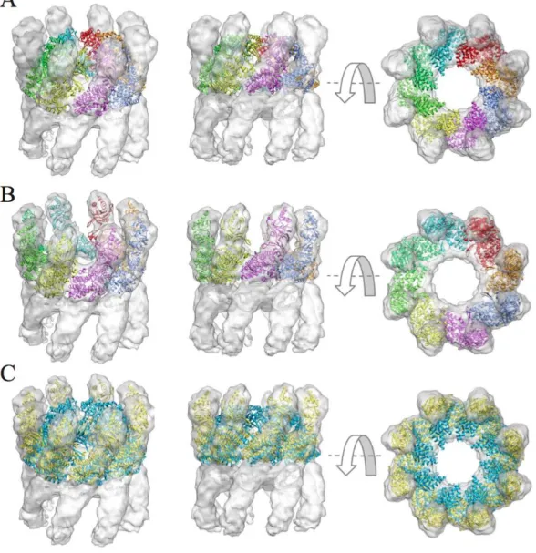
(41) Following, some flexible fittings with iMODFIT in combination with ADP_EM are presented:. Figure 10: Flexible fitting of the thermosome into an experimental EM map at 10Å. Panel A shows the initial orientation obtained with ADP_EM, in B, the model adjusted with iMODFIT, and in C, the overlap of the initial structure (blue) on the model (yellow). The map is displayed in transparency.. 33.

(42) Figure 11: Flexible fitting of the GroEL into an experimental EM map at 10 Å In panels A and B two side views of the initial structures (blue) and adjusted (yellow) are shown, respectively. In C the initial structure aligned on the final structure with Chimera is shown.. As previously mentioned, it is frequent to first perform a rigid body fitting (ADP_EM) and then adjust the conformations by applying a flexible fitting (iMODFIT) for greater accuracy.. 34.

(43) The following is an image illustrating this case:. Figure 12: Flexible fitting of the RepB in the presence of DNA using iMODFIT. The orientation of the initial structure (panel A) has been determined with ADP_EM. Panel B shows the final model of the flexibly fitted obtained with the default parameters. Arrows indicate the regions that require flexible fitting.. 35.

(44) 3. Results 3.1 Chimera UCSF Chimera is a 3D visualization program for EM density maps and atomic structures. This program includes a suite of tools for interactive analyses of sequences and structures. In particular, it offers interaction with molecular structures and related data, including supramolecular assemblies, molecular dynamics trajectories, and multiple sequence alignments. Moreover, it enhances researcher workflow with novel extension features and the creation of HD images and animations for publication and presentation purposes.. Figure 13: A snapshot of the UCSF Chimera program.. Besides supporting 3D visualization, other native features include: • Multiscale Models assemblies.. to. visualize. large-scale. • ViewDock to screen docked ligand orientations.. 36. molecular.

(45) • Volume Viewer to visualize density maps. • Multalign Viewer to display sequence alignments, with crosstalk to any associated structure. Chimera is distributed with full documentation and a number of tutorials. It can be downloaded free of charge for academic, government, non-profit, and personal use. It is available for several platforms, including Windows, MacOS X, and Linux. Chimera is developed and supported by the Resource for Biocomputing, Visualization, and Informatics, and it is funded by the NIH National Center for Research Resources at the University of California, San Francisco. The software is specifically designed for extensibility, to allow outside developers to incorporate new desirable functions. The principal objective of this work has been the development, optimization, and adaptation of the ADP_EM and iMODFIT tools to be integrated as plugins in Chimera.. 3.2 ADP_EM Plugin for Chimera The main objective of this project is the development of two plugins for Chimera to perform the two types of fitting (rigid and flexible), this is, ADP_EM and iMODFIT. Both of them conserve the same parameters and features as the original methods but are easier to use. Furthermore, the user can interactively visualize the different solutions as soon as they are computed. In this section, the ADP_EM plugin for Chimera is presented. The ADP_EM plugin developed for Chimera is located in a newly created EM Fitting section in the Tools menu that Chimera offers to the users (Figure 14).. 37.

(46) .. Figure 14: ADP_EM entry menu in Chimera.. When ADP_EM is loaded, the basic window or GUI that is presented to the user is shown (Figure 15):. Figure 15: ADP_EM basic GUI in Chimera.. As it can be seen, the most important parameters of the original methods are readily available in the basic window. The first field selects the atomic structure and the second is the map. The rest of them are described below: • Bandwidth: it corresponds to the bandwidth in the harmonic transformation. Its values are set to 16, 24, 32, 48 or 64. They correspond to increasing angular sampling values.. 38.

(47) • Resolution: the nominal resolution of the projection map [Å]. • Cut-off: is the density threshold value for the experimental map. All density levels below this value will be not considered. User can get this value from Volume Viewer dialog through the Get from Volume Viewer button available. These parameters are the minimum required to perform the fitting. The next ones are advanced features that should be used carefully by the user: • Fitting criterion: this option sets the fitting criterion: o Standard cross-correlation  the scalar product between the density map of the low resolution map and the low-pass filtered atomic structure. Recommended for resolutions < 15 Å, specially the atomic model accounts all the density of the map. o Laplacian filter  is applied by default to maximize the fitting contrast. Recommended for resolutions  15 Å, specially when the atomic model only accounts a part of the density of the experimental map. • Saved solutions: number of the saved solutions that ADP_EM will compute (50 by default). • Translational sampling: in [Å], by default twice of voxel size of the density map. Values > 6 Å should not be used. • Translational scan: translational scan strategy: o Full search  all the translational points inside the target EM map will be explored. o Limited  radial search starting from the center of mass. o Masking search  by default.. 39.

(48) Apart from the button that displays the options for expert users, there are four more: • Fit: performs the fitting after validating properly the parameters. • Results: displays the solutions of the fitting in a new panel. It is disabled while fitting is being performed. • Close: close the GUI but keeps all the values associated. • Help: opens a help guide in the browser. Once the user has loaded the atomic structure and the map and inserted coherent values for the basic parameters, the fitting can be performed by clicking the Fit button (Figure 16). When the ADP_EM is executed, a new window is shown to the user with the process log and a progress bar to check the status (Figure 17).. Figure 16: ADP_EM GUI status just before perform fitting. EM map and atomic structure are loaded and the minimum required parameters are set.. 40.

(49) Figure 17: ADP_EM fitting process shown by the log window.Notice how all the buttons are disabled while the process is running.. In addition to these parameters, some extra features had been provided to expert ADP_EM users (Figure 18). These parameters can be found in the Options button, that are displayed in a new panel: • Number peaks explored per docking: default 30. • Number peaks stored per iteration: default 20. • Number peaks stored in the search: default 100. • Number peaks stored in the multi-docking search: default 500. • Translational threshold in grid units: default 2.0. • Rotational threshold in degrees: default 360/bandwidth. • Width between spherical layers: default 1.0. • Density cut-off of the simulated map: default 0.0. 41.

(50) Figure 18: ADP_EM expert GUI in Chimera.. Mainly, the execution time varies depending on the Bandwidth value. The finer the angular sampling (bandwidth), the more it takes.. Figure 19: ADP_EM process finished.Notice how all the buttons are now enabled.. 42.

(51) Once the process is finished, the log informs that the user can check the solutions (Figure 19), and the user can visualize the solutions in the Results panel which can be seen in Figure 20:. Figure 20: ADP_EM Results panel with all the calculated solutions dropped down.. As it can be seen, the main options keep visible to let the user perform another fitting if it is necessary. Apart of this, there is a drop-down menu to choose one of the solutions computed by ADP_EM. When one of them is chosen, the opened atomic structure updates its coordinates and moves into the map to the fitted position calculated by ADP_EM (Figures 21, 22 and 23).. 43.

(52) Figure 21: ADP_EM Solution 1 fitted into the map.. Figure 22: ADP_EM Solution 8 fitted into the map.. 44.

(53) Figure 23: ADP_EM Solution 10 fitted into the map.. Additionally, a button called Save Solution was implemented to make a copy, with a representative name, to the Model Panel of the chosen solution. Model Panel is a very important dialog of Chimera that shows to the user all the models opened in the program (Figure 24).. Figure 24: Copies of solutions 1, 8 and 10 and molecule positioned in solution 17.. 45.

(54) The last button in the Results panel, Back to initial, simply resets the coordinates of the molecule and moves it to the original position it had before the fitting was performed. Briefly, the Help button opens a user guide in the browser with instructions to load correctly the plugin in Chimera and a description of the parameters involved to use them properly.. Figure 25: A snapshot of the user guide.. It is very common that users, once they loaded the atomic structure and the map, move the molecule for some analytic reasons. This situation had to be considered during the plugin development because it involves camera motions related to the objects as well as changes in their internal coordinates.. Figure 26: Objects loaded (A) and objects moved (B).. 46.

(55) This had added considerable difficulty in achieving the plugin but it maintains its efficiency and maintainability.. Figure 27: Solution 16 of the moved molecule from Figure 25b.. In later chapters the dissemination of this plugin will be described as well as the different guides and considerations for its correct usage.. 3.3 iMODFIT Plugin for Chimera The iMODFIT plugin is located (with ADP_EM) in the newly created EM Fitting section of the Chimera Tools panel (Figure 28). It can be used (and should be) with some of the solutions provided from ADP_EM in a previous execution.. 47.

(56) Figure 28: iMODFIT entry menu in Chimera.. When iMODFIT is loaded, the basic window or GUI that is presented to the user is shown below (Figure 29):. Figure 29: iMODFIT simplest GUI in Chimera.. As can be seen, there are many options for the user to perform the flexible fitting that match the original parameters of the method. The first field selects the atomic structure to fit in the map, the second one. The rest of them are described below: • Resolution: the resolution criterion follows EMAN package procedures. It is the nominal resolution of the projection map in [Å]. • Fix DoF: randomly fixed ratio of dihedral coords. Example: 0.7 = 70% of dihedrals will be randomly fixed. User can choose between None, 50% (fast), 70% (faster) or 90% (fastest).. 48.

(57) • Cut-off: is the density threshold value for the experimental map. All density levels below this value will be not considered. User can get this value from Volume Viewer dialog when the map is loaded through the button available. • Model: represents the coarse-grained model. User can choose between Heavy-atoms, C5 or Cα (as described in 2.3) • Number of modes and % Mode: Used modes range, either number [1,N] <integer>, or ratio [0,1) <float> (default=0.05). Apart from the button that displays the options for expert users, there are four more: • Fit: performs the fitting after validating properly the parameters. • Results: displays the solutions of the fitting in a new panel. It is disabled while fitting is being performed. • Close: close the GUI but keeps all the values associated. • Help: opens a help guide in the browser. Once the user has loaded the atomic structure and the map and inserted coherent values for the minimum parameters, the fitting can be performed by clicking de Fit button (Figure 30). When the iMODFIT is executed, a new window is shown to the user with the process log (Figure 31).. 49.

(58) Figure 30: iMODFIT GUI status just before start fitting. EM map and the first solution of ADP_EM are loaded and the minimum required parameters are set.. Figure 31: iMODFIT fitting process shown by the log window. Notice how all the buttons are disabled while the process is running.. In addition to these parameters, some extra features had been provided to expert users. These parameters can be found in the. 50.

(59) Options button, which displays a new panel to insert them (Figure 32):. Figure 32: iMODFIT expert GUI in Chimera.. • Introduce options: this field allows user introduce advanced commands for iMODFIT. Example: --addnevs 0.2 –pdb_ref chainX.pdb • Rediagonalization: RMSD ratio to trigger diagonalization. Default 0. User can choose between None, 0.1, 0.5 or 1. Mainly, the execution time varies depending on the values of the parameters. Usually, iMODFIT takes several minutes to perform the flexible fitting.. Figure 33: iMODFIT process finished. Notice how all the buttons are now enabled.. 51.

(60) Once the process is finished, the log informs that the user can check the solutions (Figure 33), and the user can visualize the solutions in the Results panel which can be seen in Figure 34:. Figure 34: iMODFIT Results panel.. Additionally, iMODFIT generates five files in the working directory: • imodfit_fitted.pdb: fitted atomic structure • imodfit_movie.pdb: multi-pdb trajectory movie • imodfit_score.pdb: score file to check for convergence • imodfit_model.pdb: original atomic structure • imodfit.log: used command log As can be seen, the main options keep visible to let the user perform another flexible fitting if it is necessary. The button Show fitted molecule switches between the original molecule and the fitted one generated (Figure 35 and 36) and enables, when showing the fitted molecule, the possibility of copying it (Figure 37 and 38).. 52.

(61) Figure 35: iMODFIT showing the original molecule.. Figure 36: iMODFIT showing the fitted molecule.. 53.

(62) Figure 37: iMODFIT showing the fitted molecule and its copy in the Model Panel.. Figure 38: iMODFIT showing the original molecule and the fitted copy.. As iMODFIT generates a multi-pdb trajectory movie, there has been included another option, Open movie, that allows the user to open this file and check all the different trajectories that were generated in the flexible fitting (Figure 39 and 40).. 54.

(63) Figure 39: Frame 9 of the trajectory movie generated by iMODFIT.. Figure 40: Frame 1 of the trajectory movie generated by iMODFIT.. 55.

(64) Briefly, the Help button opens a user guide in the browser with instructions to load correctly the plugin in Chimera and a description of the parameters involved to use them properly.. Figure 41: A snapshot of the user guide.. In later chapters the dissemination of this plugin will be described as well as the different guides and considerations for its correct usage.. 3.4 Plugins Testing In this section the different tests made for checking the correct functionality of the ADP_EM and iMODFIT plugins will be described. As described before, Chimera requires a restart every time a change its made in a plugin, so there is no way to create an isolated test to check some feature. In this context, each test is a result of making a modification in the plugin code, restarting Chimera, and testing such a change.. 1.. Open Chimera and load the ADP_EM plugin with no  data.. 56.

(65) 2.. Open Chimera and load the ADP_EM plugin with some molecule and EM map previously loaded. Check if the  objects appear in the plugin to be selected.. 3.. Open Chimera, load the ADP_EM plugin and display the  Options panel.. 4.. Open Chimera, load the ADP_EM plugin and open the  help guide in the browser with the Help button.. 5.. Open Chimera, load the ADP_EM plugin and close it  with Close button correctly.. 6.. Open Chimera, load the ADP_EM plugin with no data and try to perfom a fitting. The message Choose model  and map is shown.. 7.. Open Chimera, load the ADP_EM plugin with some molecule and EM map previously loaded and try to  perfom a fitting. The message Cutoff must be defined is shown.. 8.. Open Chimera, load the ADP_EM plugin with some molecule and EM map previously loaded and get the  cutoff level from the Volume Viewer dialog.. 9.. Open Chimera, load the ADP_EM plugin with some molecule and EM map previously loaded, cutoff  defined and try to perfom a fitting. The message Resolution must be defined is shown.. 10.. Open Chimera, load the ADP_EM plugin with some molecule and EM map previously loaded, cutoff defined, resolution defined to 70 or -2 and try to  perfom a fitting. The message Resolution must be between 0 and 59 is shown.. 11.. Open Chimera, load the ADP_EM plugin with some molecule and EM map previously loaded, cutoff  defined, resolution defined and try to perfom a fitting.. 12.. Open Chimera, load the ADP_EM plugin with all the existing parameters introduced and check that all the  values are properly set into the plugin.. 13.. Open Chimera, load the ADP_EM plugin with the minimum required parameters and some advanced  options introduced and try to perform a fitting.. 14.. Check that the process log window opens correctly and shows the ADP_EM process log when performing a  fitting. Also check the progress bar status works fine.. 15.. Check that the Fit, Options, Results and Close buttons . 57.

(66) are disabled when performing a fitting. 16.. Check that the Fit, Options, Results and Close buttons  are enabled when fitting process is finished.. 17.. Display the Results panel when the fitting process is  finished.. 18.. Check that all the ADP_EM solutions are set to the  drop-down menu in the Results panel.. 19.. Check that the molecule moves correctly to the  position of the first chosen ADP_EM solution.. 20.. Check that the molecule switches correctly its position  between different chosen ADP_EM solutions.. 21.. Check that a copy of the chosen ADP_EM solution is created in the Model Panel when Save solution button  is pressed.. 22.. Check that the copy of the chosen ADP_EM solution is  the same and is in the same position as it.. 23.. Check that ADP_EM plugin removes all temporal files  generated during the fitting process.. 24.. Check that ADP_EM plugin does not create PDBs with  the solutions and store all in memory.. 25.. Check that ADP_EM plugin creates pipes between  Chimera and the fitting process correctly.. 26.. Check that ADP_EM plugin communicates bidirectionally between Chimera and the fitting  process.. 27.. Check that ADP_EM can load files from different  locations and perform the fitting correctly.. 28.. Check that ADP_EM communicates properly with  Chimera native dialogs.. 29.. Check that ADP_EM is able to make another fitting when a previous one is finished and the Results panel is  being displayed.. 30.. Check that data stored in memory from a previous fitting is properly cleaned to ensure a correct  functioning when performing a new one.. 31.. Check that ADP_EM prevents Chimera blocking when  performing a fitting.. 32.. Open Chimera and load the iMODFIT plugin with no  data.. 58.