Contaduría y Administración 63 (2), Especial 2018, 1-20 Accounting & Management
* Corresponding author.
E-mail address: daniel.sotelsek@uah.es (D. Sotelsek)
Peer review under the responsibility of Universidad Nacional Autónoma de México. http://dx.doi.org/10.22201/fca.24488410e.2018.1188
0186- 1042/© 2018 Universidad Nacional Autónoma de México, Facultad de Contaduría y Administración. This is an open access article under the CC BY-NC-ND (http://creativecommons.org/licenses/by-nc-nd/4.0/)
A generic fiscal rule: Proposal and design
Propuesta y diseño de una regla fiscal genérica
Guido Zack
aand Daniel Sotelsek
b*
aUniversidad de Buenos Aires and Universidad Nacional de San Martín, Argentina bUniversidad de Alcalá, Spain
Received 8 August 2016; accepted 5 December 2016 Available online 30 May 2018
Abstract
The State has two essential tools to achieve the goal of macroeconomics stability, monetary policy and
fiscal policy. However, the progress in terms of behavioral rules has been greater in the case of monetary
policy. This article aims to make a contribution in relation to the mechanism that should be followed by a
fiscal rule to promote a counter-cyclical behavior, without questioning the solvency of the public sector. To do so, the flexibility of the rule is fundamental, through a proper selection of its base and a clear and transparent escape clause. Once described its desirable characteristics, a generic fiscal rule is proposed,
which has to be adapted to each particular case. This is done for the case of Spain in the years prior to the
last crisis. Finally, it is concluded that a well-designed fiscal rule can be really useful not only for purposes
of solvency and stability but also as a guide for discretion.
JEL Classification: E32, E62, H60.
Key words: Fiscal policy, Rules, Discretion, Solvency, Stability.
Resumen
Las herramientas esenciales del Estado para cumplir con el objetivo de estabilidad macroeconómica
un aporte en relación al mecanismo que debería regir una regla fiscal, de forma que fomente un compor
-tamiento contracíclico, sin que ponga en cuestionamiento la solvencia del sector público. Para ello, es fundamental dotar a la regla de flexibilidad, a través de una correcta selección de la base y una cláusula de escape clara y transparente. Una vez descritas sus características deseables, se propone una regla fiscal genérica que debería ser adaptada a cada caso particular, en esta oportunidad el ejercicio se realiza para el caso de España en los años previos a la última crisis. Finalmente, se concluye que una regla fiscal bien
diseñada puede ser de mucha utilidad no solo para los objetivos de solvencia y estabilidad, sino también como guía para la discrecionalidad.
Códigos JEL: E32, E62, H60.
Palabras clave: Política fiscal, Reglas, Discrecionalidad, Solvencia, Estabilidad.
Introduction
If we want to review the history of economic theory and its policy recommendations, it is best
to keep track of the discussion on how the state should act in the face of economic fluctuations. While both monetary and fiscal policy are considered essential to possible government action,
they have undoubtedly been the focus of attention for a long time. Even towards the end of the 20th century, the view that central banks should be independent and that there should be
an explicit monetary policy rule in the style of the Taylor rule prevailed. However, in the case of fiscal policy, the issue has never been very clear. Beyond the recommendation of having a balanced budget or not, there is no vocation to coordinate a fiscal rule to be followed by the
different economies; there is not even a consensus on whether it should exist in the same way
as the monetary rule. In this sense, this article considers that the phenomenon of the fiscal rule,
its design and possible implementation, has not been fully analyzed, and that the indicators on
which it is based in many cases have had flaws that have undermined its credibility
Developing such a rule is no easy task. Therefore, this article analyses the desirable
characteristics of any fiscal rule, and then makes a specific proposal and a framework for its practical application. To this end, the following section includes a definition of a fiscal
rule, indicating the reasons for which its introduction was considered relevant, including the
incentive to deficit and the procyclicality that governments possess. In the third section, a series
of trade-offs are presented with which the rules have to deal with, both in their two most important objectives and in their main characteristics. The different options regarding the rule
design are then developed, in particular concerning the base and escape clauses. In the fifth
section, a rule is proposed, which should be adapted to each particular case. To this end, an application exercise is carried out for Spain in the years prior to the 2008 crisis, using the SFR estimate created by Zack et al. (2014). Finally, the final considerations are presented.
Definition, background, and reasons for fiscal rules
A fiscal rule is defined as any legislative element that conditions the conduct of fiscal policy
(Debrun et al., 2008: 300) expressed in terms of a long-term performance indicator, such as
deficit, indebtedness, or one of the main components of these indicators (Kopits and Symansky,
Its earliest history dates back to the mid-nineteenth century, when many states in the United States took on the responsibility of adopting a new golden rule1 (Buchanan, 1997: 119). After
the war, this golden rule became explicit in several of the defeated countries (Germany, Japan,
and Italy) as part of their stabilization programs. Thus, the first experiences had as their sole and exclusive objective fiscal discipline (Kopits, 2001: 4-5). While subsequent rules maintain
this objective, as they arise from the excessive debts accumulated in the 1970s and 1980s, they also include stabilization targets and transparency standards to monitor their effective implementation (Debrun et al., 2008: 305).
On this occasion, the rules seem to have been more widely accepted, as the number of countries using them to guide their policy has increased from seven in 1990 to eighty twenty
years later (IMF, 2009: 7-9). Of course, this figure is influenced by supranational rules, which
are present not only in the European Union, since the entry into force of the Maastricht Treaty in 1992 and the Stability and Growth Pact in 1997, but also in the currency unions of Eastern Caribbean, West Africa, and Central Africa (Schaetcher et al., 2012: 10-14). However, in the European Union, almost all members complement the European framework with their own rules (European Commission, 2009: 87-93).
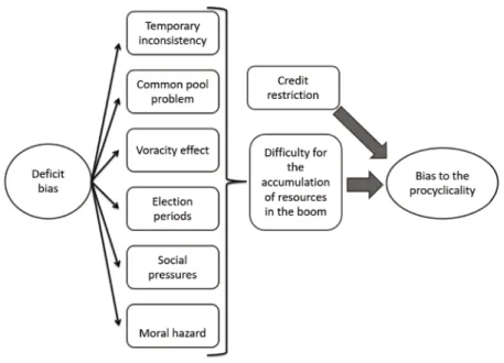
Now, why are fiscal rules necessary? There are a number of reasons for this, including a bias towards deficit and procyclicality in discretionary behavior. The delay in the implementation of fiscal policy also plays a very important role, while the creation of monetary unions raises the need for it to be accompanied, at the very least, by some fiscal coordination (see Figure 1).
Figure 1: Incentives for deficit and procyclicality
Source: Own elaboration based on Debrun et al. (2008).
Deficit bias
Monetarists argue that both monetary policy (Friedman, 1968) and fiscal policy (Barro,
1974) are incapable of having a long-term impact on real economy. For this reason, they propose
as optimal fiscal policy the one that keeps the tax rate constant, that is, they eliminate the use
of discretionary measures, leaving the task of stabilization to monetary policy and automatic
fiscal stabilizers (Friedman, 1948: 247-250; Barro, 1979: 941-950; Lucas and Stockey, 1982). However, with some exceptions, some authors do recognize the capacity of both types of
policies to generate short-term effects. Therefore, just as monetary policy has an incentive to be
expansive in order to promote employment at the cost of higher possible inflation (Nordhaus, 1975), fiscal policy has a bias towards deficit (Kydland and Prescott, 1977: 473-474; Buchanan, 1997: 120-123; Halac and Yared, 2014).
This bias is reinforced in certain situations, such as elections. Given that voters are not aware of the intertemporal budgetary constraint (Corsetti and Roubini, 1993: 63-70), the Government
has an incentive to deviate from the optimal fiscal policy, with the objective of increasing the
level of activity and employment, thus raising its positive image (Buchananan and Wagner, 1977: 114-115; Cukierman and Meltzer, 1986; Poterba, 1994: 816-818)2. The incentive for diversion
is not limited to the level of public spending, but also includes its composition by increasing consumption-related items and reducing investment-related items (Rogoff, 1990: 21).
Even during non-electoral periods, the common pool problem shows that certain items of public expenditure can be used to favor certain groups of interest (Weingast et al., 1981: 650-651; Velasco, 1997: 4).
Procyclicality bias
The common pool problem also generates a tendency towards pro-cyclicality. Indeed, in
times of boom, tax revenues are plentiful, while there are opportunities for private profit, which increases the incentive to lobby. Thus, additional fiscal resources are not used to reduce deficit
or debt in order to be better prepared for a reversal of the cycle (Lane and Tornell, 1996 and 1998; Tornell and Lane, 1998; Lane, 2002). This voracious effect may explain why both in
Europe (European Commission, 2001: 63-64) and in other developed countries (Hercowitz and
Strawczynski, 2004; Balassone and Francese, 2004) the procyclical character is concentrated during booms, while in recessions there is usually a behavior that is rather acyclical (Manasse, 2006: 15-19).
While there is evidence of procyclical fiscal policies in various regions of the world3, this
bias is reinforced in developing countries (Talvi and Vegh, 2005; Alesina and Tabellini, 2005),
in part because credit constraints prevent them from running fiscal deficits during the recession
(Kaminski et al., 2004).
On the other hand, the typical volatility of these economies is reflected on the tax bases,
ultimately impacting collection. In this way, any attempt to soften intertemporal public spending
would mean incurring large surpluses during booms and significant deficits in recessions. However, as economies with large unmet social needs, the pressures to allocate surpluses for 2 The generation of deficits not only increases their chances of remaining in power, but—if they lose—it leaves less resources for the next government (Persson and Svensson, 1989; Alesina and Tabellini, 1990).
this purpose are very significant, so it is not so easy to generate savings in the boom (Talvi and
Vegh, 2005: 177-180).
Membership of a monetary union and the delay in implementation
A monetary union implies a single monetary policy and as many fiscal policies as there
are members of the union. Nothing ensures that all these policies are compatible with those developed by the Central Bank (Buti et al., 2001). Indeed, there is reason to argue that the
deficit incentive is higher in these cases. First, the incorporation into a common monetary
space generates a decrease in interest rates in many countries, which encourages indebtedness
and allows high fiscal deficits to be incurred (Buti and Giudice, 2002: 2-4). Second, given the
interconnection between countries and the damaging spillover effects of the eventual default of a member, the possibility of being rescued creates a moral hazard that may encourage national
authorities to incur larger deficits (Inman, 1996: 2-3). Third, since it is not in charge of monetary policy, political short-sightedness does not allow us to see the adverse effects of a larger deficit
on inflation (Beetsma and Uhlig, 1999: 553)4.
Having ceded monetary (and exchange rate) policy to a supranational central bank, a very important challenge for the design of fiscal rules arises: to be sufficiently rigid to avoid excessive deficits, but also sufficiently flexible to reduce volatility.
Even governments that have a strong reputation and are not expected to have the biases
outlined above have incentives to implement fiscal rules. The reason for this is the time it usually takes to implement a discretionary measure in fiscal policy (Kopits, 2001: 8; Wyplosz, 2005: 81-82). In fact, several quarters may elapse from the identification of the need until the
measure takes effect (Blanchard and Perotti, 1999, 13-16).
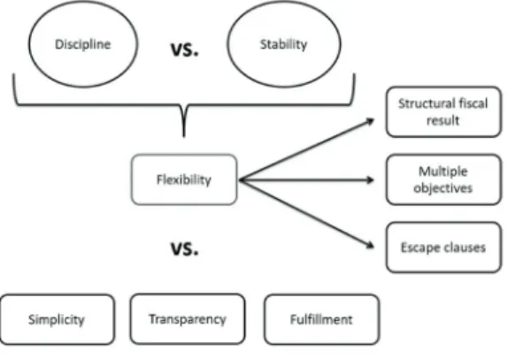
Trade-offs of fiscal rules
Once the possible costs of discretion have been raised, a series of trade-offs arise in the
implementation of fiscal rules (see Figure 2).
Figure 2: Trade-offs of fiscal rules
Source: Own elaboration based on Kopits and Symansky (1998).
The first is the one that occurs between the objectives of discipline and stability. This is because, while a tight fiscal policy would be effective in terms of increased solvency, it would also have a lower response to fluctuations in the economic cycle (Eichengreen, 1992: 30-32;
Poterba, 1994: 812-816; Alt and Lowry, 1994: 823-824; Bohn and Inman, 1996: 40-46; Lane, 2003: 5-6).
However, all these studies analyze only one side of the coin, as they only consider the possibility that fiscal rules restrict the countercyclical nature of policies. Conversely, there is
also the possibility that public-sector behavior tends to be procyclical, so imposing limits on it may mitigate an additional factor of volatility (Buchanan, 1997, 127-129; Debrun et al., 2008: 302-303; Alesina and Bayoumi, 1996). Even other authors conclude that the rules not only
improve fiscal performance, but also reduce macroeconomic volatility, denying the existence
of the trade-off (Ayuso-i-Casals et al., 2006: 687-691; Manasse, 2005 and 2006). Fatás and
Mihov (2005) recognize that the introduction of restrictions limits the response of fiscal policy to exogenous shocks, increasing volatility. On the other hand, a more stable fiscal policy is
generated, which more than offsets the previous effect.
From the above, it can be said that the effect of the rules on volatility is not predefined and will depend on the objective pursued by the fiscal policy: in the case of a predominantly
countercyclical character, then the limitations could accentuate the instability; on the other
hand, if the evolution of the fiscal policy is procyclical, the restrictions help achieve greater
stability.
Nevertheless, there is one more factor to consider. The deficit bias may even cast doubt on
the solvency of the State (Buchanan, 1997: 120-123). In this case, access to the capital market
is seriously hampered and countercyclical fiscal policy is often prevented, especially during
downturns (Aizenman et al., 1996; Gavin and Perotti, 1997; Catao and Sutton, 2002; Kaminski et al., 2004).
However, one way to combine the positive effect of the rule on discipline, without limiting the countercyclical capacity, is to give the rules flexibility. There are several ways to make a rule capable of reacting to economic cycle movements. The first is to establish the restriction on a long-term indicator, such as the structural fiscal result (SFR), rather than the observed fiscal result (OFR), thus leaving the automatic stabilizers in operation (Kopits and Symansky, 1998: 24-25). Another way, as will be seen below, is to apply the rule to more than one fiscal indicator
(Ter-Minassian, 2010: 11-12; Schaechter, et al. 2012: 15-16) or to vary the target fiscal outcome along with the economic cycle.
But even flexible rules could generate counterproductive constraints in cyclical terms in
exceptional situations of strong external shocks. For these cases, there are so-called escape
clauses, which define the conditions that must be met for the rule to be temporarily suspended
and for the limits imposed by it to be exceeded. These conditions, as well as those that restore
rule operation in the event of temporary suspension, must be explicitly defined in advance, as
well as easily supervised.
In short, a sufficiently flexible rule could circumvent the possible trade-off between solvency and stability. However, the lower rigidity of the restrictions poses a major challenge to the design of the rule and a new trade-off, as introducing flexibility in the rule necessarily
implies making it less simple and transparent, which in turn makes enforcement more difficult5.
A flexible rule loses simplicity on the basis of having to be applied to more than one
objective, because the objectives are more complex, and because of the inclusion of escape clauses. Even more so if these objectives change from being observed indicators, such as
expenditure, income, fiscal performance or debt, to estimated indicators, such as the SFR.
Flexibility, on the other hand, leads to much greater demand in terms of transparency
(Cangiano, 1996). Although the publication of the relevant information of the fiscal accounts in time and form is always fundamental (Kopits and Craig, 1998: 7-9), this task becomes more
demanding as it has to be done with indicators that are not observed, but estimated, and even projected (Buti et al., 2003: 20-21).
Finally, given that simplicity and transparency are essential for the supervision of the
rule and its effective compliance (Kopits and Craig, 1998: 19), the greater demand and eventual deterioration of these characteristics could affect enforcement and, consequently, the
effectiveness of the restrictions in obtaining its solvency and stability objectives (Tanzi, 1993).
Design of fiscal rules
Considering the biases to the deficit and procyclicality of discretionary fiscal policy, as well as the desirable features of the rules to correct them (flexibility, simplicity, transparency), below different options are developed with regard to the design of fiscal rules in relation to their
base indicator and escape clauses. The basis of the rule
The basis of the rule refers to the indicator on which the numerical restriction is made (Ter-Minassian, 2010: 10). This aspect is extremely important, as its choice conditions the response of the rule to the preservation of solvency and the maintenance of stability (Bohn and Inman, 1996: 30-34). Consideration should also be given to how controllable it is by the Government, if it is able to provide operational guidance at all times during the cycle, and the ease with
which it can be monitored (IMF, 2009: 4 and 20). The most frequent candidates are the level of indebtedness, expenditure, income, and the fiscal result.
Level of indebtedness
If the objective is to ensure the solvency of the State, the first indicator referred to is public
debt. By prohibiting the level of indebtedness from exceeding a certain percentage of the
GDP, the development of the fiscal outcome and, consequently, also of government revenue
and expenditure, is conditioned. In addition, such a rule is simple, transparent, and easy to communicate.
However, as the only instrument, it has the disadvantage that it takes some time to be influenced by changes in other fiscal variables, so it does not restrict policy in the short-term,
while being affected by factors that are not within the reach of the Government, such as the interest rate (IMF, 2009: 21). Similarly, it does not generate any guidance when debt is below
the limit. Finally, in the face of external shocks that could significantly deteriorate the level of activity and government revenues, the deficit may generate an increase in the debt ratio, forcing
Expense
Total, primary or current public expenditure is a variable that is almost perfectly defined by
the Government (particularly primary), while providing operational guidance at all times and being easy to monitor (IMF, 2009: 21). The restriction is based on limiting the nominal or real growth rate or its share of GDP.
Conditioning to cyclical behavior is best adjusted when the growth rate is used as a reference. In effect, a limit to the annual variation of expenditure imposes a restriction on any procyclical behavior during the boom or when income is increased by the evolution of a particular variable (prices of raw materials, investment in housing, etc.). At the same time, it allows for expansionary action in the recession, albeit limited.
The main shortcoming of this type of rule is that it is not directly related to solvency, since it does not include revenue objectives (Schaechter et al., 2012: 8-9). Thus, on the one hand, it
is not able to influence the level of indebtedness. On the other hand, it does not seem to be a
good option in the case of immature tax systems, since public revenues are expected to increase along with the modernization of the State and expenditures, in this context, may well increase at a similar rate to that of revenues without jeopardizing the solvency of the public sector (Machinea, 2012: 76).
Income
A rule based on public revenues usually imposes maximum and/or minimum limits on
the tax burden. In many cases they are very difficult to comply with, since fiscal revenue— unlike expenditures—does not fall under the direct control of the Government because it is
highly dependent on changes in the level of activity (Buti et al., 2003: 16). Even though the
elasticity may be greater than one, imposing a floor or ceiling on the tax burden can limit
the countercyclical nature of the tax system, being counterproductive in terms of stability (Schaechter et al., 2012: 9). They are also partial rules, leaving aside expenses, and are, therefore, unable to ensure responsible behavior in terms of solvency.
Other types of income rules are those that require a portion of the proceeds to be used for a specific purpose, often to generate savings during booms in the form of sovereign funds. They
are usually related to the presence of non-renewable resources, thus, in addition to stability, the
objective is to improve intergenerational equity (Jiménez and Tromben, 2006).
Fiscal result
After analyzing the limitations of the rules on the above variables, in view of the objectives
of solvency and stability, the need arises to act on a more complete indicator such as the fiscal
result (Sacchi and Salotti, 2015). In fact, its calculation incorporates both expenses and income,
while its behavior conditions the evolution of the debt. Thus, a balanced fiscal outcome over the whole cycle means that expenditure is placed around revenue, without generating significant
changes in the level of debt, which would in principle ensure solvency (Tapia, 2003: 39-41).
Similarly, a limit on the fiscal outcome in terms of GDP is relatively simple to monitor,
while providing constant guidance as to the direction the policy should take. The indicator is
sufficiently controllable by the Government, although there is some difficulty with cyclical
Nevertheless, a rule on this basis does not provide for certain countercyclical elements,
which in turn may cause solvency-related problems. If the objective is fixed, i.e., not changed
according to the phase of the cycle, should the constraint be met close to the limit during the boom, it is highly likely to be missed once the economy slows down as a result of the fall in revenues. In this way, in order to comply with the rule again, the Government would be forced
to consolidate the fiscal result in a clear procyclical action in the recession (Manasse, 2005:
8-11).
One option to mitigate the absence of countercyclical elements is to apply the target on the structural indicator (Ter-Minassian, 2014; Bova et al., 2014). In doing so, automatic stabilizers
are excluded from the scope of the rule (Ter-Minassian, 2010: 8-11). However, as seen since the
2008 crisis, this indicator is not satisfactory in identifying income from asset revaluation. To this end, it is very useful to develop a structural indicator that does consider these effects, such as the one developed by Zack, et al. (2014)6.
Although, even if you want to enhance the stabilizing effect of fiscal policy, without having
to resort to escape clauses or break the rule, you can consider some kind of mechanism in
which the target level varies throughout the cycle. One possibility is that the objective is a fixed
percentage of the Output Gap (OG). Thus, during booms, when GDP is above potential, the target SFR would be positive. Conversely, in recessions, where the OG is negative, the same
rule would allow a structural deficit to be incurred.
Combination of bases
Another alternative to cover both the solvency and stability objective is to develop a rule that
combines different bases. The most frequent combinations are restrictions on fiscal expenditure
or result, with limits on the level of indebtedness.
As seen above, the level of indebtedness is a good indicator to encourage more responsible attitudes in terms of solvency, but in many cases, it does not generate any kind of guide for
fiscal policy, and at the same time it does not imply important restrictions in cyclical terms.
Expenditure, on the other hand, is useful for stability purposes, especially when its rate of change is limited, but because it does not take into account income, it is unable to act on solvency as a
whole. Thus, a combination of both indicators could include the two final objectives, without
generating a highly complex rule and maintaining their transparency (Schaechter, 2012: 9). The main limitation of this combination is that it still does not directly consider income. One way to include income more directly is by combining the debt target with another SFR target (Ter-Minassian, 2010: 11-12). It should be noted that this combination is the one originally chosen by the European Union for its members, although recent experience, in many cases, has not produced the expected results.
There could even be a rule in which the objective of the base fluctuates with the cycle, so
as to promote the stabilizing effect. On the other hand, the level of indebtedness, together with
the possible existence of contingent liabilities, could define the value above which the target
level would vary. In the case of a country with low debt and no contingent liabilities that wants to maintain or even increase its level of debt, this value could be zero or negative, respectively (Blanchard et al., 1990: 10-12; Cuddington, 1997: 6-8). However, in a country where the debt is
above the allowed maximum, or where there is a real probability of having contingent liabilities (Tapia, 2003: 39-41), this value could be positive and higher the more it surpasses the limit. Escape clauses
The basic idea of designing a rule on a cyclically fluctuating SFR objective, with flexibility
and considering the level of indebtedness and contingent liabilities, is to minimize the need to
temporarily suspend the rule. However, no design can be so complete as to previously consider
all possible scenarios that may arise. Thus, escape clauses must always be included in the rule.
This poses a major design challenge, related to the identification of those exceptional moments. An effective method of identification is essential to allow the use of flexibility and
to prevent attempts to circumvent it simply for short-term gain, without consideration for long-term solvency. Furthermore, once the decision to temporarily suspend it has been taken, the
return should be specified, as well as the treatment of the accumulated deviations (IMF, 2009:
26). As will be seen in the following section, the proposed generic rule and its application in the
Spanish case has an escape clause designed (Equations 1 and 2). The basic idea is to condition the deactivation and subsequent reactivation to a certain value (in this case the OG) to be defined by governments on a case-by-case basis.
Generic proposal for a fiscal rule and its application to the case of Spain
Having developed the motivations that encouraged the introduction of fiscal rules, their
desirable characteristics, possible trade-offs and the alternatives in relation to their design, a generic rule model is proposed below.
The proposed fiscal rule sets out its objective indicator in a combination of bases already
mentioned above: the SFR and the level of indebtedness. The former is used as the most comprehensive indicator, including both tax revenue and expenditure. In particular, its structural
version is used, so that a first level of flexibility is given by allowing the automatic stabilizers
to operate freely.
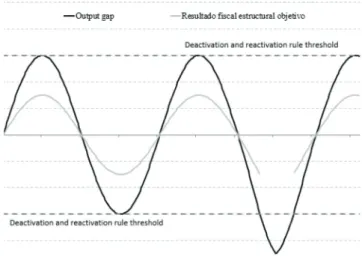
Additionally, to accentuate its flexibility and stabilizing capacity, it is proposed that the objective base fluctuates with the cycle. The simplest and most immediate option for this is for limitations to the SFR value to be a positive fixed percentage of the OG. Thus, when the
economy is booming, the SFR objective will be greater than zero, generating savings. On the other hand, in a contractionary part of the cycle, the OG is negative and, therefore, so is the SFR objective, allowing the public sector to boost demand (Figure 3).
The solvency objective implies that the cyclical fluctuations of the SFR should be centered on zero, that is, a long-term budgetary balance is envisaged. However, depending on the level of indebtedness, the possibility of contingent liabilities or other justified reasons, this value
could be different. Thus, in the event of over-indebtedness, under the threat of a natural disaster,
or due to the ageing of the population, for example, the center of the fluctuations on the SFR
could be positive, with the aim of generating savings. On the other hand, in the event of a very low debt situation, the center could be temporarily negative.
the suspension is due to a recession, then discretion should be directed towards a higher deficit.
The reactivation of the rule would occur once the OG returns to the values set as thresholds. In the event that the borrowing exceeded the limit value due to the countercyclical policy, then the
requirement that the center of the fluctuations be positive would be activated, thus generating
the process of debt reduction. On the other hand, if the boom had generated savings considered
excessive to meet any type of contingency, then a medium-term deficit could arise until the
level of indebtedness or the amount of the desired sovereign wealth fund is reached. In this way, the operating mechanism itself provides a guide to the treatment of deviations generated at times when the rule is deactivated.
In this manner, the formula of the rule is the following:
Where SFR is the structural fiscal outcome; ‘x’ is the long-term objective or the center of cyclical fluctuations of the SFR; ‘y’ is the permitted or required percentage of short-term deviation from the long-term objective; OG is the output gap; and ‘z’ is the threshold for the
deactivation and reactivation of the rule.
Figure 3: General operation of the rule
Source: Own elaboration based on Ter-Minassian (2010) and Schaechter et al. (2012).
The case of Spain prior to 2008: an application exercise
The first step in applying this rule to the Spanish case is to have a good SFR indicator. For this purpose, the first option would be to take the estimate of the European Commission. However, while this methodology may capture some of the cyclical components of income and
expenditure, it does not consider extraordinary income from asset revaluations, and is subject to large ex-post corrections, so basing a policy decision on this indicator is very risky.
In turn, the SFR will be used for Spain, estimated by Zack et al. As can be observed in Table
fact that it considers the extraordinary public revenues generated by the housing bubble and the
construction boom. This indicator identifies that the fiscal deterioration in Spain began towards the beginning of the 2000s and already in 2004 it showed a structural deficit of the order of 4
percentage points of GDP. On the other hand, for the SFR of the European Commission, as well
as for the OFR, the fiscal deterioration only began in 2007 and it was not until 2008, when the crisis began, that the first deficit was observed.
Once we have a good SFR indicator, we proceed to set the parameters of the rule. For Spain
in the years prior to 2008, an appropriate percentage for the target value of SFR (“y” in Equation
1) is considered to be 50% of the OG. Thus, for example, when the GDP exceeds potential by
1%, then an SFR of 0.5% of potential GDP will be required, plus automatic stabilizers to obtain
the OFR. On the other hand, in the face of a recession in which the GDP is 2% below potential,
the rule itself will make it possible to incur a structural deficit of 1% of potential GDP, to which
automatic stabilizers should again be added. With regard to the average target value (“x”), it is considered that Spain did not face an over-indebtedness situation nor a need to generate long-term savings7. A balanced budget is thus envisaged in the medium term. As for the escape
clause, the thresholds for the suspension and reactivation of the rule are set at 3% and -3% OG, respectively. Thus, it is considered that Spain has not experienced any situation in the years
prior to the crisis that justifies the suspension of the rule.
In short, the formula of the rule for Spain would be as follows:
Where SFR is the structural fiscal result and OG is the output gap
Next, the calculation of the additional fiscal savings that Spain would have achieved
between 2000 (when it joined the Monetary Union) and 2008 (the year in which the crisis began) if it had complied with a rule of this nature is carried out8. As can be observed in Table
1, these resources would have reached 48.5% of the GDP. Even if the SFR estimated by the European Commission had been considered, instead of the one calculated by Zack et al. (2014), the additional savings would have been 25% of the GDP.
7 A valid reason for Spain to consider the need to generate a long-term surplus of resources is the deficit in social security, especially in relation to retirement and pension funds, in the face of an ageing population.
Table 1
Application of the fiscal rule to Spain (% of the GDP)
Output Gap Objective of structural fiscal result according to the rule Structural fiscal result according to Zack et al. (2014)
Additional savings in case of having adjusted to the rule
Structural fiscal result according to the European Commission Additional savings in case of having adjusted to the rule
2000 3.06 1.53 -2.37 3.90 -2.26 3.79
2001 3.36 1.68 -2.41 4.09 -2.36 4.04
2002 2.74 1.37 -2.94 4.31 -1.89 3.26
2003 2.32 1.16 -3.59 4.75 -1.62 2.78
2004 2.11 1.05 -4.44 5.49 -1.18 2.23
2005 2.29 1.14 -4.18 5.32 -0.03 1.17
2006 2.99 1.49 -4.04 5.54 0.59 0.91
2007 3.04 1.52 -4.36 5.88 0.36 1.16
2008 1.32 0.66 -8.57 9.23 -5.14 5.80
Total 48.50 25.14
Source: Own elaboration based on the European Commission (2009) and Zack et al. (2014).
Thus, had the proposed rule been applied in Spain since 2000, the country would have
started the crisis with a very interesting flow of resources. This, on the one hand, would have
cooled the economy in the years leading up to the crisis, causing some effect on the housing bubble. More importantly, however, it would have been possible to implement a more powerful countercyclical policy once the crisis had begun. In effect, following the proposed escape clause, the rule would have been temporarily suspended in 2009, as the OG was -3.3% of the potential GDP. In this way, there would have been free reign of discretion to carry out measures to boost aggregate demand, beyond what is allowed by the rule.
In short, this exercise shows the importance of a fiscal rule designed ad hoc (in a context of
monetary union). An effective SFR indicator, which clearly identifies extraordinary revenues, is essential for this. Otherwise it would be very difficult to withstand the pressures to expand public spending when the rule required an observed surplus.
Finally, a clarification: what has been done in this section is a partial fiscal policy exercise.
Thus, it is not unknown that the proposed measures would have had effects on other economic
variables, which could have modified the scenario. Nor does it argue that fiscal policy alone
could have prevented the crisis. Conversely, the exercise is only intended to show that different
fiscal behavior in cyclical terms would have been not only prudent, but also desirable in the
interest of the real stability of the economy.
Conclusions
Firstly, the discussion on the role of the State in the economy is not a fact defined or
contrasted by empirical evidence. The 2008 crisis undoubtedly supports the intervention, but what is really interesting is to emphasize it during periods of stability and growth, when no one has incentives to ruin the party and, therefore, countercyclical policies are expected.
A second point is the pre-eminence of the study and analysis of monetary policy and the
conclusion on the need to follow predetermined rules. Meanwhile, on the fiscal side, although there has been much debate about the consequences of their behavior, little progress has been made in deepening a fiscal rule.
Although there is evidence that the application of a rule encourages countercyclical fiscal
policy behavior (Bergman and Hutchison, 2015; Grembi et al., 2016; Alberola et al., 2016),
there is less consensus on the design of the rule. This is why, in the first part of the article, after mentioning the existing incentives for the application of fiscal rules, its design options have been analyzed. Thus, first of all, the main trade-offs were reviewed, among which stand out discipline vs. stability and flexibility vs. simplicity, transparency, and compliance with the rule. Subsequently, taking these trade-offs into account, the actual design options were studied. In this way, the different possible bases—indebtedness, expenditure, revenue, observed or structural fiscal result, or some combination of these—were considered, as well as the need to
provide the rule with clear and transparent escape clauses, but also to consider the situation that would automatically reactivate the functioning of the rule.
Once the design options were analyzed, a generic rule proposal was made based on a combination of the SFR and the level of indebtedness, using the OG as a guide for temporary
suspensions and reactivations of the rule. Furthermore, in order to make it more flexible, it was suggested that the objective should not be fixed, but that it should fluctuate with the OG. Thus, the rule requires not only a surplus observed in the boom, but a structural surplus as well; and the same for the deficit during the recessionary phases. It should be noted that this
increased stabilizing capacity does not undermine the solvency objective, as it calls for a balance throughout the entire cycle.
This generic rule is not intended to limit, but to serve as a guide for discretion and good
management of aggregate fiscal accounts. That is why the definition of the parameters of Equation (1) is left to each particular case. In this way, each government can define its
long-term (parameter “x”) and short-long-term (parameter “y”) objectives, according to their own vision
of the current state of its economy and the desired goal. Similarly, it can define which cases
are considered exceptional to allow the rule to be deactivated (and automatically reactivated; parameter “z”).
In this sense, the aim of this work is the design and proposal of the fiscal rule, while
previous work (Zack et al., 2014) focused on analyzing and estimating a central variable such as the SFR, whose methodological summary can be seen in Annex I. Precisely, the exercise for the case of Spain (in the years prior to the last crisis) aims to test the functioning of the rule based on the SFR estimated in the previous work. To this end, parameters “x”, “y” and “z” are
defined, according to the situation in Spain up to 2008, characterized by low indebtedness and
a long upward cycle (see Annex II). The application of this rule would have allowed savings
equivalent to almost half the GDP of 2008 (if the SFR were used considering asset revaluation) or to one quarter (if the asset revaluation was not considered).
If Spain had had those resources, its policy response to the crisis experienced between 2008
other words, the rule would have allowed for more countercyclical fiscal behavior, generating
greater savings in the boom (helping avoid a larger bubble), in order to use those resources
during the recession (helping avoid such a significant fall in output and such a pronounced
unemployment rate).
Finally, it should be made clear that the application of a rule is usually the result of prior
consensus on the need to develop a more responsible fiscal policy, and not the beginning of it.
Whether or not Spain was in a position to apply such a rule at the beginning of this century is
beyond the scope of this article, although it is not trivial that it has achieved a fiscal surplus in
2006 and 2007. In the same way, any country whose objective is the implementation of the rule
must first analyze whether the conditions are met, both in the political and social spheres. In other words, the rule hardly generates the countercyclical behavior of fiscal policy, but rather
vice versa, the rule is often the institutionalization of responsible behavior.
References
Aizenman, J., Gavin, M., & Hausmann, R. (1996). Optimal Tax Policy with Endogenous Borrowing Constraints.
NBER Working Paper, 5558.
Alberola, E., Kataryniuk, I., Melguizo, Á., & Orozco, R. (2016). Fiscal policy and the cycle in Latin America: the role of financing conditions and fiscal rules. Documentos de trabajo del Banco de España, 1604.
Alesina, A. & Tabellini, G. (2005). Why is Fiscal Policy Often Procyclical? NBER Working Paper, 11600.
Alesina, A., & Bayoumi, T. (1996). The Costs and Benefits of Fiscal Rules: Evidence from U. S. States. NBER Working
Paper, 5614. https://doi.org/10.3386/w5614
Alt, J. & Lowry, R. (1994). Divided Government, Fiscal Institutions, and Budget Deficits: Evidence from the States.
The American Political Science Review, 88(4), 811-828. http://dx.doi.org/10.2307/2082709
Ayuso-i-Casals, J., González Hernández, D., Moulin, L. & Turrini, A. (2006). Beyond the SGP – Features and Effects
of EU National-Level Fiscal Rules. Preparado para el 2006 Public Finance in EMU European Commission Report, The Role of National Fiscal Rules and Institutions in Shaping Budgetary Outcomes, Bruselas, 24 de noviembre. https://doi.org/10.1057/9780230271791_10
Balassone, F. & Francese, M. (2004). Cyclical Asymmetry in Fiscal Policy, Debt Accumulation and the Treaty of Maastricht. Banca d’Italia, Temi di Discussione, 531. Barro, R. (1974). Are Government Bonds Wealth? Journal of Political Economy, 82, 1095-1117. https://doi.org/10.1086/260266
Barro, R. (1979). On the Determination of the Public Debt. Journal of Political Economy, 87(5), 940-71. https://doi. org/10.1086/260807
Beetsma, R. & Uhlig, H. (1999). An Analysis of the Stability and Growth Pact. Economic Journal, 109, 546-571. http:// dx.doi.org/10.1111/1468-0297.00462
Bergman, U. M., & Hutchison, M. (2015). Economic stabilization in the post-crisis world: Are fiscal rules the answer? Journal of International Money and Finance, 52, 82-101. https://doi.org/10.1016/j.jimonfin.2014.11.014
Blanchard, O., Chouraqui, J-C., Hagemann, R. & Sartor, N. (1990). The sustainability of fiscal policy: new answers to an old question. OCDE Economic Studies, 15. https://doi.org/10.1787/021121358375
Blanchard, O. & Perotti, R. (1999). An Empirical Characterization of the Dynamic Effects of Changes in Government Spending and Taxes on Output. NBER Working Paper, 7269. https://doi.org/10.3386/w7269
Bova, E., Carcenac, N., & Guerguil, M. (2014). Fiscal rules and the procyclicality of fiscal policy in the developing
world. IMF Working Paper, 122. https://doi.org/10.5089/9781498305525.001
Bohn, H. & Inman, R. (1996). Balanced Budget Rules and Public Deficits: Evidence from the U.S. States. NBER
Wor-king Paper, 5533. https://doi.org/10.3386/w5533
Buchanan, J. (1997). The balanced budget amendment: Clarifying the arguments. Public Choice, 90(1), 117-138. http://dx.doi.org/10.1023/A:1004969320944
Buti, M., Roeger, W. & In´t Veld, J. (2001). Stabilizing Output and Inflation: Policy Conflicts and Co-operation under
a Stability Pact. Journal of Common Market Studies, 39(5), 801–828. http://dx.doi.org/10.1111/1468-5965.00332
Buti, M. & Giudice, G. (2002). EMU’s Fiscal Rules: What Can and Cannot Be Exported. Preparado para la conferencia
Rules-Based Fiscal Policy in Emerging Market Economies, IMF - World Bank, Oaxaca, Mexico, 14-16 de febrero. https://doi.org/10.1057/9781137001573_7
Buti, M., Eijffinger, S. & Franco, D. (2003). Revisiting the Stability and Growth Pact: grand design or internal adjust
-ment? European Economy, Economic Papers, 180.
Cangiano, M. (1996). Accountability and Transparency in the Public Sector: The New Zeland Experience. IMF Wor-king Paper, 122. https://doi.org/10.5089/9781451854442.001
Catao, L., & Sutton, B. (2002). Sovereign Defaults: The Role of Volatility, IMF Working Paper, 149. https://doi. org/10.5089/9781451856903.001
Chamorro Narváez, R. A., & Urrea Bermúdez, A. F. (2016). Effects of fiscal rules on regional public debt sustainability
in Colombia. Cuadernos de Economía, 35(SPE67).207-251. http://dx.doi.org/10.15446/cuad.econ.v35n67.52461 Corsetti, G. & Roubini, N. (1993). The Design of Optimal Fiscal Rules for Europe After 1992. En F. Torres y F.
Giavazzi (Eds.), Adjustment and Growth in the European Monetary Union (pp. 46-82). Cambridge: Cambridge University Press. https://doi.org/10.1017/cbo9780511599231.006
Cuddington, J. (1997). Analysing the sustainability of fiscal deficits in developing countries. Georgetown University,
Economics Department. http://inside.mines.edu/~jcudding/papers/Sustain/Sustainability(9.3.99).pdf https://doi. org/10.1596/1813-9450-1784
Cukierman, A. & Meltzer, A. (1986). A Positive Theory of Discretionary Policy, the Cost of Democratic Government
and the Benefits of a Constitution. Economic Inquiry, 24(3), 367-388. http://dx.doi.org/10.1111/j.1465-7295.1986. tb01817.x
Debrun, X., Moulin, L., Turrini, A., Ayuso-i-Casals, J. & Kumar, M. (2008). Tied to the mast? National fiscal rules in
the European Union. Economic Policy, 23(4), 297-362. http://dx.doi.org/10.1111/j.1468-0327.2008.00199.x
Eichengreen, B. (1992). Should the Maastricht Treaty Be Saved?. Princeton Studies in International Finance, 74.
Eichengreen, B. & von Hagen, J. (1995). Fiscal Policy and Monetary Union: Federalism, Fiscal Restrictions and the
No-Bailout Rule. CEPR Discussion Paper, 1247. https://doi.org/10.3386/w5517
European Commission (2000). Public Finance in EMU – 2000. European Economy, 3.
European Commission (2001). Public Finance in EMU – 2001. European Economy, 3.
European Commission (2009). Public Finance in EMU – 2009. European Economy, 5.
Fatás, A., & Mihov, I. (2006). The macroeconomic effects of fiscal rules in the US states. Journal of Public Economics,
90(1-2), 101-117. http://dx.doi.org/10.1016/j.jpubeco.2005.02.005. FMI (2009). Crisis and Recovery. World Economic Outlook, abril.
Friedman, M. (1948). A monetary and Fiscal Framework for Economic Stability. The American Economic Review, XXXVIII(3), 245-264. https://doi.org/10.2307/1907322
Friedman, M. (1968). The role of monetary policy. The American Economic Review, LVIII(1), 1-17. https://doi. org/10.1007/978-1-349-24002-9_11
Gavin, M., & Perotti, R. (2003). Fiscal Policy in Latin America, NBER Macroeconomics Annual, 1997, pp. 11-61. https://doi.org/10.1086/654320
Girouard, N. & André, C. (2005). Measuring Cyclically-adjusted Budget Balances for OECD Countries. OECD Eco-nomics Department Working Papers, 434. https://doi.org/10.1787/787626008442
Grembi, V., Nannicini, T., & Troiano, U. (2016). Do Fiscal Rules Matter? American Economic Journal: Applied
Eco-nomics, 8(3), 1-30. https://doi.org/10.1257/app.20150076
Hagemann, R. (1999). The Structural Budget Balance. The IMF´s Methodology. IMF Working Paper, 95. https://doi. org/10.5089/9781451851809.001
Halac, M., & Yared, P. (2014). Fiscal rules and discretion under persistent shocks. Econometrica, 82(5), 1557-1614. ht-tps://doi.org/10.3982/ecta11207
Hercowitz, Z. & Strawczynski, M. (2004). Cyclical Ratcheting in Government Spending: Evidence from the OECD.
The Review of Economics and Statistics, 86(1), 353-361. http://dx.doi.org/10.1162/003465304323023868
Inman, R. (1996). Do Balanced Budget Rules Work? U.S. Experience and Possible Lessons for the EMU. NBER
Jiménez, J. P., & Ter-Minassian, T. (2016). Política fiscal y ciclo en América Latina: el rol de los gobiernos subnacio -nales. Serie Macroeconomía del Desarrollo, 173, CEPAL.
Jiménez, J. P. & Tromben, V. (2006). Política fiscal en países especializados en productos no renovables en América
Latina. CEPAL, Serie Macroeconomía del Desarrollo, 46.
Kaminsky, G., Reinhart, C. & Végh, C. (2004). When it Rains, it Pours: Procyclical Capital Flows and Macroeconomic
Policies. NBER Working Paper, 10780. https://doi.org/10.3386/w10780
Kopits, G. (2001). Fiscal Rules: Useful Policy Framework or Unnecessary Ornament? IMF Working Paper, 145. ht-tps://doi.org/10.2139/ssrn.2094462
Kopits, G. & Craig, J. (1998). Transparency in Government Operations. IMF Occasional Paper, 158. https://doi. org/10.5089/9781557756978.084
Kopits, G. & Symansky, S. (1998). Fiscal Rules. IMF Occasional Paper, 162. https://doi.org/10.5089/9781557757043.084
Kydland, F. & Prescott, E. (1977). Rules Rather than Discretion: The Inconsistency of Optimal Plans. The Journal of
Political Economy, 85(3), 473-491. https://doi.org/10.1086/260580
Lane, P. R. (2002). The Cyclical Behaviour of Fiscal Policy: Evidence from the OECD. Journal of Public Economics, 87(12), 2661-2675. http://dx.doi.org/10.1016/S0047-2727(02)00075-0
Lane, P. R. & Tornell, A. (1996). Power, growth and the voracity effect. Journal of Economic Growth, 1(2), 213-241. http://dx.doi.org/10.1007/BF00138863
Lane, P. R. & Tornell, A. (1998). Why aren´t Latin American savings rates procyclical? Journal of Development
Eco-nomics Nº 57(1), 185-199. http://dx.doi.org/10.1016/S0304-3878(98)00082-0
Lucas, R. Jr. & Stockey, N. (1982). Optimal Fiscal and Monetary Policy in an Economy without Capital. The Cen-ter for Mathematical Studies in Economics and Management Science Discussion Paper, 532. https://doi. org/10.1016/0304-3932(83)90049-1
Machinea, J. L., Vásquez González, L. & Zack, G. (2012). La ciclicidad de las políticas públicas latinoamericanas
(1995-2010). Madrid: CeALCI - Fundación Carolina.
Manasse, P. (2005). Deficit Limits, Budget Rules, and Fiscal Policy, IMF Working Paper, 120. https://doi. org/10.5089/9781451861396.001
Manasse, P. (2006). Procyclical Fiscal Policy: Shocks, Rules, and Institutions - A View From MARS. IMF Working Paper, 27. https://doi.org/10.5089/9781451862874.001
Nordhaus, V. (1975). The Political Business Cycle. Review of Economic Studies, 42(2), 169-90. https://doi. org/10.2307/2296528
Persson, T. & Svensson, L. (1989). Why a stubborn conservative would run a deficit: Policy with time-inconsistent
preferences. Quarterly Journal of Economics, 104(2), 325-345. https://doi.org/10.2307/2937850
Phelps, E. (1961). The Golden Rule of Accumulation: A Fable for Growthmen. American Economic Review, 51(4),
638–41. https://doi.org/10.1016/b978-0-12-554002-5.50007-8
Poterba, J. M. (1994). State Responses to Fiscal Crises: The Effects of Budgetary Institutions and Politics. Journal of Political Economy, 102(4), 799-821. https://doi.org/10.1086/261955
Rogoff, K. (1990). Equilibrium Political Budget Cycles. The American Economic Review, 80(1), 21-36. https://doi. org/10.3386/w2428
Sacchi, A., & Salotti, S. (2015). The impact of national fiscal rules on the stabilisation function of fiscal policy.
Euro-pean Journal of Political Economy, 37, 1-20. https://doi.org/10.1016/j.ejpoleco.2014.10.003
Schaechter, A., Kinda, T., Budina, N. & Weber, A. (2012). Fiscal Rules in Response to the Crisis—Toward the `Ne -xt-Generation´ Rules. A New Dataset. IMF Working Paper, 187. https://doi.org/10.5089/9781475505351.001
Talvi, E. & Vegh, C. A. (2005). Tax base variability and procyclical fiscal policy in developing countries. Journal of
Development Economics, 78(1), 156 – 190. http://dx.doi.org/10.1016/j.jdeveco.2004.07.002
Tanzi, V. (1993). The Political Economy of Fiscal Deficit Reduction. En W. Easterly, C. Rodriguez & K. Schmidt-He -bbel (Eds.), Public Sector Deficits and Macroeconomic Performance (pp. 513-524). New York: Oxford University Press y World Bank. https://doi.org/10.2307/1061325
Tapia, H. (2003). Balance estructural del Gobierno central de Chile: análisis y propuestas. Serie macroeconomía del
Taylor, J. B. (2000). Remarks for the Panel Discussion on Recent Changes in Trend and Cycle. Preparado para la con-ferencia Structural Change and Monetary Policy, Federal Reserve Bank of San Francisco y Stanford Institute for Economic Policy Research, 3-4 de marzo.
Ter-Minassian, T. (2010). Preconditions for a successful introduction of structural fiscal balance-based rules in Latin
America and the Caribbean: a framework paper. Inter-American Development Bank Discussion Paper, 157.
Ter-Minassian, T. (2014). Should Latin American countries adopt structural balance-based fiscal rules? Revista de
Economía y Estadística, 49(2), 115-143.
Tornell, A. & Lane, P. R. (1998). Are windfalls a curse? A non-representative agent model of the current account.
Jour-nal of InternatioJour-nal Economics, 44(1), 83-112. http://dx.doi.org/10.1016/S0022-1996(97)00016-0
Velasco, A. (1997). A Model of Endogenous Fiscal Deficits and Delayed Fiscal Reforms. NBER Working Papers, 6336. https://doi.org/10.3386/w6336
Weingast, B., Shepsle, K. & Johnsen, C. (1981). The Political Economy of Benefits and Costs: A Neoclassical Approach
to Distributive Politics. Journal of Political Economy, 89(4), 642-64. https://doi.org/10.1086/260997
Wolf, H. (2005). Volatility: definitions and consequences. En J. Aizenman y B. Pinto (Eds.), Managing Volatility and
Crises. A Practitioner Guide (pp. 45-64). Cambridge: Cambridge University Press. https://doi.org/10.1017/cbo9780511510755.004
Wyplosz, C. (2005). Fiscal Policy: Institutions versus Rules. National Institute Economic Review, 191. https://doi. org/10.1177/0027950105052661
Zack, G. et al. (2014). Towards an Effective Structural Budget Balance for Economic Stability. Hacienda Pública Española / Review of Public Economics, 210-(3/2014): 11-31. http://dx.doi.org/10.7866/HPE-RPE.14.3.1.
Annex I: Methodology for calculating the structural fiscal result (SFR)
Faced with the need to know the fiscal situation of the States, the total or primary fiscal result is normally used. These indicators have the disadvantage of reflecting short-term and volatile income and expenditure, which are the
result of the economic cycle phase. The SFR seeks to isolate these cyclical components, leaving only the permanent or structural ones.
To this end, the phase of the economic cycle is first identified through the OG. Then, the relationship between the cycle and the fiscal result is made through the elasticities between the variation in the main income (direct taxes on
natural and legal persons, indirect taxes, and social security contributions) and expenditure, and the variation in the OG
(Equations A.2 and A.4). Each of these elasticities is, in turn, the result of the product of two elasticities. In the case of the income, the first step is to obtain the elasticity between the change in the tax base of each tax and the change in the
OG. On the other hand, the elasticity between the collection and the tax base is obtained, which is sometimes estimated and sometimes an assumption is made based on the expected behavior given the characteristics of the tax. Then, by multiplying these two elasticities, the elasticity that measures the variation in each income in the face of variations
in the OG is reached (Equation A.3). The total income elasticity is obtained by means of a weighted average of the
elasticities of each tax, according to its share in total revenue collection.
In the case of expenditure, only expenditure related to unemployment is considered cyclical. Thus, the elasticity between expenditure and OG is obtained from the product of the elasticity between the variation in the unemployment
gap (measured as the quotient between the observed unemployment rate and the NAWRU) and the variation in OG, and the elasticity between the variation in total expenditure and the variation in the unemployment gap (Equation A.5).
Once the cyclically adjusted income and expenditure are reached, subtraction is done to obtain the nominal SFR,
where the superscript “*” indicates structural value; FR is the fiscal result; Ti is the tax revenue corresponding
to category “i”; G is the public expenditure; is the expenditure related to unemployment; Y is the gross domestic product; U is the unemployment rate; is the elasticity of category “i” of income with respect to the OG; is the elasticity of the tax base of category “i” of income in relation to the OG; is the elasticity of income “i” in relation to its tax base; is the elasticity of public expenditure in relation to the OG; is the elasticity of primary public expenditure in relation to the unemployment gap; and is the elasticity of unemployment in relation to the OG.
While this methodology is capable of isolating the cyclical components of government income and expenditure, it
often has difficulty in identifying the effect of asset overvaluation (bubbles), which are not always fully reflected in the OG. To this end, a term is added to Equation A.2 that reflects the effect of the overvalued asset on different government income. Thus, Equation A.2 would be replaced by Equation A.6:
where A is the price of the overvalued asset and is the elasticity of income “i” relative to the overvalued asset.
In the specific case of Spain in the years prior to the last crisis, the SFR was calculated using this methodology,
using investment in nominal housing as an overvalued asset. This variable makes it possible to capture both the
overvaluation of house prices and the boom in construction that affected the quantities9.
Annex II:
Main economic statistics of Spain
GDP (inter-annual variation)
Observed Fiscal Result (% of the GDP)
Public income (% of the GDP)
Public expenditure (% of the GDP)
Public debt (% of the GDP)
Investment
in Housing
(% of the GDP)
Unemployment rate
(% of the EAP)
2000 5.3 -1.0 38.1 39.1 58.0 8.8 11.9
2001 4.0 -0.5 37.9 38.5 54.2 9.1 10.6
2002 2.9 -0.4 38.2 38.6 51.3 9.6 11.5
2003 3.2 -0.4 37.9 38.3 47.6 10.3 11.5
2004 3.2 0.0 38.6 38.7 45.3 10.9 11.0
2005 3.7 1.2 39.5 38.3 42.3 11.5 9.2
2006 4.2 2.2 40.5 38.3 38.9 12.1 8.5
2007 3.8 2.0 40.9 38.9 35.5 11.7 8.2
2008 1.1 -4.4 36.7 41.1 39.4 10.4 11.3
2009 -3.6 -11.0 34.8 45.8 52.7 8.1 17.9
2010 0.0 -9.4 36.2 45.6 60.1 6.9 19.9
2011 -1.0 -9.6 36.2 45.8 69.5 5.7 21.4
2012 -2.9 -10.5 37.6 48.1 85.7 4.9 24.8
2013 -1.7 -7.0 38.6 45.6 95.4 4.1 26.1
2014 1.4 -6.0 38.9 44.9 100.4 4.3 24.5
2015 3.2 -5.1 38.6 43.8 99.8 4.4 22.1