Unemployment and private returns to higher education in Argentina (1974 2002)
23
0
0
Texto completo
(2) Unemployment and private returns to higher education in Argentina (1974-2002) Cecilia Adrogué 1*. Abstract The paper analyzes the private returns to higher education in Argentina during the period 1974– 2002. The main conclusion is that returns to education are positive and increase once corrected by the level of unemployment. As a consequence, when analyzing whether to invest in education, one should not only consider as benefits the differential in earnings, but also the higher probability of having a job that comes with attaining more education. This is particularly relevant in a country like Argentina which had unemployment rates of 5% during the eighties and started to have unemployment rates in the double digits by the end of the 20th century and the beginning of the 21st century. Resumen El trabajo analiza la evolución de los retornos privados a la educación superior en Argentina durante el período 1974–2002 y cómo éstos se vieron afectados por el desempleo. La conclusión es que los retornos a la educación son mayores si se los corrige teniendo en cuenta el desempleo para cada nivel educativo, ya que a mayor nivel, menor tasa de desempleo. Al evaluar invertir en educación no se debería considerar simplemente el diferencial de ingresos sino también la mayor probabilidad de tener un trabajo. Esto es relevante en un país como Argentina que pasó de tener tasas de desempleo cercanas a 5% en la década del ochenta a tener tasas de dos dígitos a fines del siglo XX y comienzos del XXI. Keywords: Returns to higher education, unemployment JEL Classification: [I21] [J24] [J31] [J60]. 1.- Licenciada en Economía (UCA), Doctorado San Andrés, CONICET, [email protected], [email protected] * I am very grateful to Jorge Paz, Juan J. Llach, Ricardo and Jill Adrogué, Marcos Dal Bianco as well as seminar participants at AAEP, CEMA University and IAE, Austral University. All errors are mine. 32 •. ensayo 2010 (formulitas).indd 32. 5/2/11 8:42:24 AM.
(3) e n s a y o s d e p o l í t i ca ec o n ó m i ca – A ñ o 2 0 1 0. 1. Introduction Education can be considered an investment in human capital. That is the way it has been evaluated by a vast branch of the economic literature which started with Gary Becker´s work (1964). As with any other investment, education should only be carried out if the benefits are larger than the costs. However, as the investment and the benefits do not take place at the same moment in time, both should be expressed in a homogenous measure. This is done by discounting future flows by an inter-temporal discount factor or interest rate. If the inter-temporal interest rate were zero, which would mean that one peso today is the same as one peso tomorrow, then it would be enough to add up the costs and compare them with the sum of benefits. But if the inter-temporal interest rate were positive, which would mean that one peso today is preferable to one peso tomorrow, the costs and benefits flows should be discounted in order to make them homogeneous and comparable. A problem that arises when evaluating investment in education is that there is not an obvious interest rate to homogenize the flows, which makes it very difficult to calculate the present value of education, as well as almost impossible to find a price against which it can be compared. This is because there are no comparable investments regarding the risk and other unique characteristics of investing in education. The relevant literature has typically used the internal rate of return on education, that is, the interest rate that makes costs equal benefits. One major advantage of this measure is that, unlike the net present value, it is not expressed in monetary terms, i.e. it does not lose relevance as time goes on, and it is also an intuitive measure of profitability. This internal rate of return could then be compared with the rate of return of other investments in order to decide whether to carry it out. Given these considerations, we believe it to be a worthwhile effort to quantify the benefits provided by education without losing sight of the fact that many of them are very difficult to measure.. 2. Literature View Starting with Gary Becker, Jacob Mincer and Theodore Schultz’s contributions, the demand for education has been studied as an investment in human capital, and its returns estimated (Harmon et al., 2003). The two most common methods used to estimate returns to education have been the Mincer´s equation and the calculation of the internal rate of return. Both methods are equivalent under the following two assumptions: a) the only cost of studying is the opportunity cost of not being in the labor market and, b) the wage differentials among workers with different schooling are stationary (Margot, 2001). This theory of human capital assumes that the amount of education, s, is chosen so as to maximize the expected future value of the stream of future incomes w, up to retirement date T, net of the costs of education cs. The optimal s is the one for which the marginal income of an additional year of schooling equals the marginal cost of that year.. At the optimum:. (1). fac ultad. ensayo 2010 (formulitas).indd 33. de. c ie nc ias. e c o n ó m i c a s. • 33. 5/2/11 8:42:24 AM.
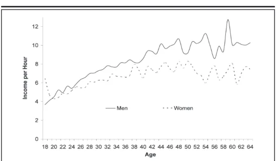
(4) Where r is the rate of return. If T is large, then the left hand side of the equilibrium relationship can be approximated so that the equilibrium condition becomes: (2). If cs is sufficiently small, we can rearrange the expression to give: (3). Where ≈ means “approximately equal to...” One could then estimate the returns to s by analyzing how the log of earnings varies with changes in s. Mincer (1974), who did one of the first empirical studies analyzing the returns to education, used an equation that relates income (wi) with years of education (si), experience (xi), squared experience (xi2 ) and other observed variables that affect income, different from experience and education (Xi). The term referred to as the “squared experience” was introduced to capture the concavity of the earnings profile, as can be observed in Figure 1. Figure 1- Income per Hour by Age for Men and Women, for All the Educational Levels. In pesos of 2002.. Source: Author’s calculation based on the EPHs.. (4) The term ui is a random error term or disturbance and represents other forces which may not be explicitly measured and that also affect the individual’s earnings. When studying the returns to 34 •. ensayo 2010 (formulitas).indd 34. 5/2/11 8:42:24 AM.
(5) e n s a y o s d e p o l í t i ca ec o n ó m i ca – A ñ o 2 0 1 0. education there could be the risk that the disturbance term may be related to some of the explanatory variables and with the explained variable. In the case at hand, both the years of education (explanatory variable) and the earnings (explained variable) depend on the abilities of the person which, since it is not an explanatory variable, is contained in the disturbance term. In this situation problems of endogeneity arise and the estimations by Ordinary Least Squares regressions are not reliable. That is, a phenomenon not attributable to education is captured by the equation. The literature refers to the reality that higher earnings could actually be due to the fact that those who pursue higher education are generally cleverer as “screening hypothesis” or “sheepskin hypothesis,”2 which may be the reason behind the positive correlation between earnings and education. In other words, there could be a problem of endogeneity and schooling may not be exogenous (Glewwe 2002). In line with the screening hypothesis, Hungerford and Solon (1987) demonstrate the existence of nonlinearity, a wage premium over the average return to schooling for fulfilling a particular year of education, for example the last year of college or high school. This shows that schooling can be used as a way to send a signal to the job market that one is smart. Following on Hungerford and Solon (1987), Spence (1973) analyzes the allocative efficiency of the job market and stresses the role of schooling as a signal. Layard y Psacharopoulos (1974) found, however, that the rates of returns of uncompleted courses were as high as those of completed courses, that standardized educational differentials rise with age even though employers have better information about older employees´ abilities, and concluded that if screening is the main function of education, it could be done more cheaply by simpler testing procedures. A number of studies have found that higher earnings are due to the fact that the individuals that continue studying acquire more cognitive skills. One of them is Boissiere et al. (1985), who examined urban wage earners in Kenya and Tanzania and found that education raises wages by providing workers with cognitive skills. Their data does not support the alternative hypothesis that education primarily reflects innate ability or sheepskin effects. Although these estimates of the returns to education have been the most commonly used, they leave out spillover effects. Education has multiple effects on the individual’s life and on society as a whole, over and above the monetary ones (Glewwe, 2002), effects that are excluded in the type of analysis discussed above. Recognizing these shortcomings, several studies have found evidence that education also contributes to economic growth (Krueger y Lindahl, 2001) and raises productivity (Sianesi y Reenen, 2003). Even more, schooling has been shown to be a key variable to determine the wage differentials among the population. It could either narrow the gap and improve the income distribution, in the case of equal educational opportunities, or widen it and make the situation worse, if those who have the possibility to study are just a few. This does not seem to happen only within countries, but also across countries, although evidence of the latter is still sparse.. 3. Returns to Education This paper intends to study the return to schooling through the calculation of the private benefits that derive from it, those that are appropriated directly by the student. In particular, we will ana-. 2.- The screening effects are increases in income solely due to the possession of a diploma or other certificate, different from the ones derived from the skills acquired during the schooling process that the certificate or diploma represents. fac ultad. ensayo 2010 (formulitas).indd 35. de. c ie nc ias. e c o n ó m i c a s. • 35. 5/2/11 8:42:24 AM.
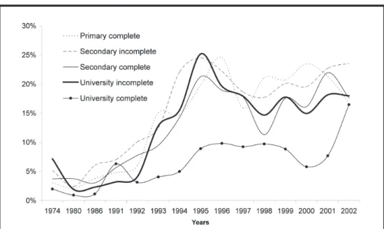
(6) lyze how those benefits are modified when one uses expected earnings instead of simple earnings in the forecasting equations. The expected earnings are calculated by multiplying the income data times the probability of having a job. The latter is a conditional probability that takes into account the age, gender and the schooling level when evaluating the incidence of unemployment. As can be observed in Figures 2 and 3, the unemployment is higher for the less educated.. Figure 2- Unemployment Rate for Men, for Each Educational Level.. Source: Author’s calculation based on the EPHs.. 36 •. ensayo 2010 (formulitas).indd 36. 5/2/11 8:42:25 AM.
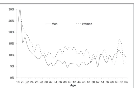
(7) e n s a y o s d e p o l í t i ca ec o n ó m i ca – A ñ o 2 0 1 0. Figure 3- Unemployment Rate for Women, for Each Educational Level.. Source: Author’s calculation based on the EPHs.. The methodology being proposed is not exempt from endogeneity problems. As the effect of the innate abilities cannot be isolated from the earnings, part of the returns attributed to education, may actually be due to ability. However, certain elements mitigate this problem. On the one side, more capable individuals tend to have higher income and therefore tend to produce an overestimation of the returns, but, at the same time, they have higher opportunity costs of studying, which partially compensates for the income effect (Harmon et al., 2003). Moreover, in Argentina the sheepskin effect is partially mitigated by the often called “brain flight” (“fuga de cerebros”), that is, the tendency of smarter Argentines to migrate because they have better opportunities abroad. In order to calculate the return to the investment in education it is essential to know its costs and benefits. Among the former affecting net returns there are direct costs, such as public expenditure in education, private donations, tuition costs, books, materials and transport costs paid by the student, as well as indirect costs, essentially the opportunity cost of not being in the labor force. Though when considering this cost, one should take into account the probability of getting a job instead of studying. As can be seen in Figure 4, unemployment is particularly high for people under 22 years old.. fac ultad. ensayo 2010 (formulitas).indd 37. de. c ie nc ias. e c o n ó m i c a s. • 37. 5/2/11 8:42:25 AM.
(8) Figure 4- Unemployment Rate by Age for Men and Women, for all the Educational Levels.. Source: Author’s calculation based on the EPHs. Costs could also be classified as social or private, depending on whether the one who pays for them is the person who is being educated or not. That is to say, even if public education is free from an individual standpoint and considering direct costs alone, it does not mean that it is costless, as the State is the one that provides for the costs; therefore, these direct costs should be taken into account in order to calculate the social returns, though not when estimating the private ones. Similarly, benefits can be classified as private and social. Private benefits are those that accrue to the educated person, while social benefits, also called externalities, refer to the gain to society which results an individual’s education. Private benefits are very important for the family’s decisions, while the latter are the ones that should guide the governmental decisions, as they capture the effect of having a more educated population. Recently in the literature, a new type of costs and benefits have been incorporated, those called fiscal costs and benefits (OECD, 2005). The former include public direct and indirect expenditures on education, as well as lost income tax revenues on students’ foregone earnings. The benefits include increased revenues from income taxes on higher wages.3 These are particularly useful so. 3.- In practice, the achievement of higher levels of education will give rise to a complex set of fiscal effects on the benefit side, beyond the effects of wage-based revenue growth. For instance, better educated individuals generally experience superior health status, lowering public outlays on the provision of health care. And, for some individuals, achieving higher levels of educational attainment may lower the likelihood of committing certain types of crime, which, in turn, would reduce public expenditure. However, tax and expenditure data on such indirect effects of education are generally unavailable. 38 •. ensayo 2010 (formulitas).indd 38. 5/2/11 8:42:25 AM.
(9) e n s a y o s d e p o l í t i ca ec o n ó m i ca – A ñ o 2 0 1 0. as to have a precise notion of how much the State is recovering from its investment in education since they allow the calculation of the fiscal internal rate of return. There are basically two methods to estimate the returns to education. The first one is the static method that uses data of a certain moment in time, which means cross section information, in order to infer the earning profile of an individual from the earnings of other people with similar characteristics. If data are only available for a unique moment in time, the static method is the only alternative to get the earnings profile of the people in the sample. The static method was the one used by Mincer. The second method is the dynamic method that uses time series in order to have the earnings profile of a certain individual derived from the observed earnings for that person analyzed at different points in time. The main advantage of this way of calculating the returns is that there is no need to infer the earnings, as in the previous method. But a major disadvantage is that it is more prone to suffer endogeneity, that is, that some characteristics of the individual which are difficult to isolate econometrically may affect the estimations. These two methods could also be seen as estimations ex ante and ex post. If one needs to decide whether to invest or not, there is no alternative than to take the expected return, but, if one is interested in the returns one got with a certain investment, one should do the calculation ex post, knowing exactly how much it cost and how much was recovered.. Figure 5- Earnings profile, comparison of the dynamic and static method. As could be seen in Figure 5, the static and dynamic estimations can differ. In the case of Argentina using the dynamic method is not an option, making the inference unavoidable. This is due to the limitations of the available surveys. Specifically, the period for which there is information does not allow for the construction of a whole income profile for an individual and it is not necessarily the same person that is interviewed in the different surveys since half of the sample is replaced each time. For this reason we have decided to use the static method, although we recognize its limitations as ignoring changes in the earnings profile due to economic growth, technological fac ultad. ensayo 2010 (formulitas).indd 39. de. c ie nc ias. e c o n ó m i c a s. • 39. 5/2/11 8:42:26 AM.
(10) change, commercial openness, or other. In Argentina the earnings profile is descending, which would suggest that the static method might overestimate the returns. The 2001 and 2002 crisis depressed earnings quite substantially but the recovery in incomes that followed should have dampened the overestimation.. Figure 6- Income per Hour for Men, for each educational level. In pesos of 2002. Source: Author’s calculation based on the EPHs.. 40 •. ensayo 2010 (formulitas).indd 40. 5/2/11 8:42:26 AM.
(11) e n s a y o s d e p o l í t i ca ec o n ó m i ca – A ñ o 2 0 1 0. Figure 7- Income per Hour for Women, for each educational level. In pesos of 2002. Source: Author’s calculation based on the EPHs.. 4. Data and Methodology The database used is the Permanent Household Survey (EPH, Encuesta Permanente de Hogares) which is undertaken by the National Institute of Statistics (INDEC). It contains educational, working, and socioeconomic information of the people living in the city of Buenos Aires and Greater Buenos Aires.4 Information is available for the months of October 1974, 1980, 1986 and 19922002. For the intermediate years no information for the people less than 25 years of age was available, and after 2002 the database has changed.5 The internal rate of return was estimated from information corresponding to individuals between 18 and 64 years of age with different schooling levels (secondary complete, university dropout and university graduate). Even though results were obtained for men and women, we considered the information for men to be more reliable, since many women are not in the labor force. 4.- The only information available for the period was the one corresponding to Buenos Aires and Greater Buenos Aires. The rest of the urban areas of the country were progressively introduced to the survey since 1992 but, in order to make comparisons, it was necessary to use a homogeneous data base. Anyway, the area of Buenos Aires and Greater Buenos Aires represents more than 50% of the urban country population, therefore, it has a great weight in the whole average. Notwithstanding that, recent studies including the rest of the country regions indicate that the internal rates of returns to education of the area of Buenos Aires may overestimate the corresponding ones to Argentina, though they present the same trend. 5.- The EPH used to be carried out twice a year, in May and October, but during 2003 a major methodological change was implemented by INDEC, including changes in the questionnaires and in the frequency of the survey visits. Because of this change, the research was done up to the year 2002. fac ultad. ensayo 2010 (formulitas).indd 41. de. c ie nc ias. e c o n ó m i c a s. • 41. 5/2/11 8:42:26 AM.
(12) probably due to non-economic factors (such as maternity), exogenous to what we are trying to measure. As a result, women’s returns would be biased downwards relative to those of men as their earnings become spotty. Harmon et al. (2003) found evidence supporting this assertion; countries with the highest rates of female participation have the lowest differences in schooling returns while countries with the lowest participation rates have amongst the largest. Another area where information was considered to be unsatisfactory was that of university dropouts. Even if the estimates for the incomplete university level were calculated, the results were less robust than those corresponding to the complete level.6 We therefore centered the analysis solely on the latter. The evolution of the returns to education is analyzed during a period of deep economic and social transformations in Argentina (1974-2002). During this period Argentina experienced a number of crises and institutional changes. Non-democratic governments (1976-1983) were followed by democratic ones. During 1989-1990 the country suffered from hyperinflation which was followed by a period of economic stability and increasing commercial openness that ended with the 2001-02 depression. The unemployment rate varied widely during these times. Some periods were characterized by low unemployment rates and others by very high ones, allowing the period of study to be divided in two sub-periods. The first one, characterized by low unemployment rates, lasted from 1974 until the beginning of the 1990s. The second one, when unemployment rates were above 10%, began in 1993. With these macroeconomic factors in mind we now proceed to analyze the returns to education empirically. Figure 8- Unemployment Rate in Argentina. 1974-2002.. Source: INDEC.. 6. One should bear in mind that this group includes either those who finished only one subject of the career as those that did not finish because of one exam. 42 •. ensayo 2010 (formulitas).indd 42. 5/2/11 8:42:26 AM.
(13) e n s a y o s d e p o l í t i ca ec o n ó m i ca – A ñ o 2 0 1 0. 5. Rates of Return to Education, 1974-2002 a. Costs Estimation No reliable estimates of the direct costs of education exist for the period under analysis. Expenditure surveys are recent and there have been large variations in relative prices during the period being analyzed. For these reasons we have left aside direct expenditures on education and have focused on the indirect costs alone, under the assumption that those who study are not part of the labor force, and therefore the opportunity cost they have is given by the income that a person their age and previous educational level that is in the labor force receives. As such, the indirect cost for a university student is the forgone earnings of a worker that has completed secondary school. Working age was assumed to start at age 18, normalizing to zero the opportunity cost prior to that age. Also, achieving a university degree was assumed to take six years; for estimation purposes, university dropouts were arbitrarily assigned four years of university schooling. Although the assumption that those who study do not work may seem too strong, it is not so once one takes into account that those who work and at the same time study, generally take longer to graduate and earn lower salaries than after graduation. The income differential and extra time in school make our estimate a good approximation for the actual opportunity cost.. b. Benefits Estimation The principal benefit that derives from having a higher level of schooling is the earnings differential. The net benefits are thus considered to be the difference between the earnings of two consecutive schooling levels.. fac ultad. ensayo 2010 (formulitas).indd 43. de. c ie nc ias. e c o n ó m i c a s. • 43. 5/2/11 8:42:26 AM.
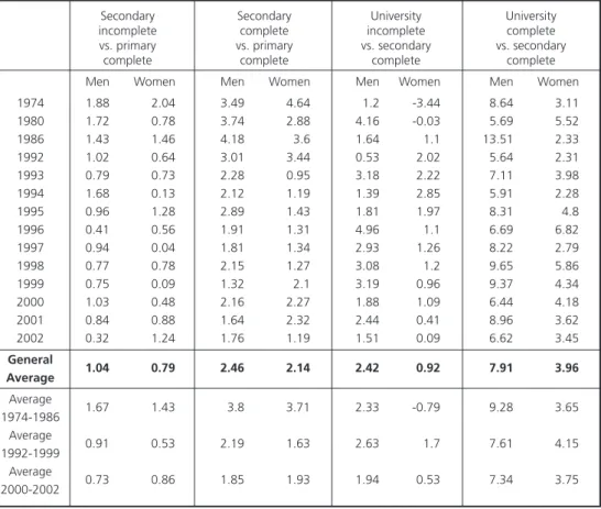
(14) Table 1- Earnings Differentials per Hour for Men and Women, for Each Educational level. In pesos of 2002. Secondary incomplete vs. primary complete . Secondary complete vs. primary complete. University incomplete vs. secondary complete. University complete vs. secondary complete. Men. Women. Men. Women. Men. Women. Men. Women. 1974 1980 1986 1992 1993 1994 1995 1996 1997 1998 1999 2000 2001 2002. 1.88 1.72 1.43 1.02 0.79 1.68 0.96 0.41 0.94 0.77 0.75 1.03 0.84 0.32. 2.04 0.78 1.46 0.64 0.73 0.13 1.28 0.56 0.04 0.78 0.09 0.48 0.88 1.24. 3.49 3.74 4.18 3.01 2.28 2.12 2.89 1.91 1.81 2.15 1.32 2.16 1.64 1.76. 4.64 2.88 3.6 3.44 0.95 1.19 1.43 1.31 1.34 1.27 2.1 2.27 2.32 1.19. 1.2 4.16 1.64 0.53 3.18 1.39 1.81 4.96 2.93 3.08 3.19 1.88 2.44 1.51. -3.44 -0.03 1.1 2.02 2.22 2.85 1.97 1.1 1.26 1.2 0.96 1.09 0.41 0.09. 8.64 5.69 13.51 5.64 7.11 5.91 8.31 6.69 8.22 9.65 9.37 6.44 8.96 6.62. 3.11 5.52 2.33 2.31 3.98 2.28 4.8 6.82 2.79 5.86 4.34 4.18 3.62 3.45. General Average. 1.04. 0.79. 2.46. 2.14. 2.42. 0.92. 7.91. 3.96. 1.67. 1.43. 3.8. 3.71. 2.33. -0.79. 9.28. 3.65. 0.91. 0.53. 2.19. 1.63. 2.63. 1.7. 7.61. 4.15. 0.73. 0.86. 1.85. 1.93. 1.94. 0.53. 7.34. 3.75. Average 1974-1986 Average 1992-1999 Average 2000-2002. Source: Author’s calculation based on the EPHs.. This paper takes this simple calculation one step further by also considering expected earnings adjusted for the incidence of unemployment. Two estimations will be performed. One considers actual earnings of employed workers. The other one adjusts these by the probability of being employed; that is multiplying actual earnings by the conditional employment rate given age, gender and schooling level.. 44 •. ensayo 2010 (formulitas).indd 44. 5/2/11 8:42:26 AM.
(15) e n s a y o s d e p o l í t i ca ec o n ó m i ca – A ñ o 2 0 1 0. Table 2- Probability of Employment for Men and Women, for Each Educational Level. In Percentage Year . Primary complete. Secondary incomplete. Secondary complete. University incomplete. University complete. Men. Women. Men. Women. Men. Women. Men. Women. Men. Women. 1974 1980 1986 1991 1992 1993 1994 1995 1996 1997 1998 1999 2000 2001 2002. 99.0 98.2 96.0 94.9 93.3 90.6 88.5 83.3 81.7 85.8 86.9 86.4 84.3 74.9 75.2. 96.9 97.9 96.2 95.2 94.0 84.9 85.3 80.2 75.5 84.1 78.9 79.3 76.5 78.7 83.1. 98.6 97.1 96.3 96.8 94.1 93.4 90.3 87.0 84.5 89.3 89.3 86.7 87.1 80.4 76.4. 94.8 97.6 94.0 93.0 89.9 87.5 77.9 75.5 77.8 81.4 82.3 79.9 80.5 77.3 76.5. 97.8 98.3 95.2 93.2 95.2 94.1 89.7 85.6 87.2 90.3 91.5 87.9 89.2 78.9 83.2. 96.3 96.2 97.0 94.4 92.3 90.5 85.7 78.7 81.1 82.2 88.7 82.4 83.9 78.1 82.4. 99.3 99.2 97.6 95.5 93.3 95.6 94.2 92.3 86.5 88.5 93.8 88.0 87.8 82.3 83.8. 92.8 98.1 97.7 96.8 96.0 87.2 84.5 74.8 80.4 82.1 85.3 82.2 85.0 81.9 82.0. 100.0 98.7 98.0 97.9 98.3 94.3 93.8 95.0 91.6 94.9 97.2 89.9 96.6 93.9 95.8. 98.0 99.1 98.9 93.7 96.9 95.9 95.0 91.1 90.2 90.8 90.3 91.2 94.2 92.3 83.5. General Average. 87.0. 85.1. 89.0. 83.8. 90.0. 86.8. 92.0. 86.4. 96.0. 93.4. 96.3. 96.4. 96.7. 94.8. 95.6. 95.9. 97.4. 97.5. 98.2. 97.2. 87.1. 82.8. 89.3. 81.5. 90.2. 85.2. 91.5. 84.1. 94.4. 92.7. 78.1. 79.4. 81.3. 78.1. 83.8. 81.4. 84.6. 83.0. 95.4. 90.0. Average 1974-1986 Average 1992-1999 Average 2000-2002. Source: Author’s calculation based on the EPHs.. c. Private rates of return As stated before, private rates of return are calculated leaving aside the externalities produced by education. Even though a number of studies have analyzed the social rates of return to education by using the earnings before taxes as opposed to the private returns that consider the disposable income (after taxes), the Permanent Household Survey database used in this study has information on disposable income (Llach, 1996) alone. Moreover, the costs analyzed here exclude public expenditure in education and private donations, only viewing the opportunity cost to the student. Finally, the results we present should be viewed as the marginal benefits to education, only valid at an individual level. This means that they are not necessarily true if all the people with a certain schooling level decided to continue studying to the following level. It may happen that as the supply of trained labor force increases, and the demand for them stays constant, the level of earnings may actually fall, and possibly, the unemployment rate for people with that level of schooling may fac ultad. ensayo 2010 (formulitas).indd 45. de. c ie nc ias. e c o n ó m i c a s. • 45. 5/2/11 8:42:27 AM.
(16) rise. As Ashenfelter and Ham (1979) state “Our results suggest that the excess of the marginal effects of schooling and experience on earnings over their effects on wage rates is due almost entirely to the effect of schooling and work experience in reducing measured unemployment... Of course, this does not imply that increased educational attainment will necessarily reduce aggregate unemployment, because the effect we observe may come merely from a redistribution of unemployment among workers.” Though Ashenfelter and Ham’s (1979) assertion should not be taken lightly, it could also happen that when a large share of the population studies, innovation increases and the ability of the enterprises to incorporate new technology also rises, pushing up economic growth. This may produce an even greater increase in the demand for the more educated than the increase in supply pushing earnings higher instead of lower. The evidence that human capital increases productivity is compelling. Studies that analyze education as a signal, such as Spence (1973), do not deny positive effects on productivity. Sianesi and Van Reenen (2003) found that a one year increase in average education is found to raise the level of output per capita by between three and six percent, and increase one percentage point the growth rate.. d. Estimating the internal rate of return to education The annual internal rate of return was calculated from the following equation applied to each educational level:. (5). r: IRR, what we want to calculate. t: Age of the individual. T: 64 years old, age at which the person retires. C: cost of education, in this case it is the opportunity cost. w: Earnings obtained by an individual with a certain educational level (j). e: age at which a certain educational level is started. In the case of higher education, it is equal to eighteen. E: age at which a certain educational level is completed (in this paper we have assumed 18 years of age for a high school graduate, 22 for university dropout and 24 for university graduate). J: educational level attained. As the information about earnings for individuals older than 18 years old is more reliable than for those aged between 12 and 17, only the opportunity cost for university students, either those who graduated or those who dropped out was calculated, but not for secondary graduates. In table 3 the values of the internal rate of return for both men and women are presented, and it 46 •. ensayo 2010 (formulitas).indd 46. 5/2/11 8:42:27 AM.
(17) e n s a y o s d e p o l í t i ca ec o n ó m i ca – A ñ o 2 0 1 0. can be seen that the latter are always lower than the former; except for the year 2002 in which the IRR of women was 16% while the corresponding to men was 15%. It should be recalled, though, that the data for men is more reliable because it does not have the noise of entry and exit from the labor force that characterizes the information for women. As shown in the table as well, the return for the complete university level is always higher than the corresponding one for the incomplete level, for all the years studied. Table 3- Internal Rates of Return to Education*. In Percentage Year 1974 1980 1986 1992 1993 1994 1995 1996 1997 1998 1999 2000 2001 2002. University incomplete 5.0 10.9 6.8 7.5 10.2 14.1 7.3 8.0 8.9 10.0 12.8 8.5 16.5 8.7. Men University complete 11.1 14.1 11.9 13.7 14.9 15.9 14.7 16.2 15.7 15.7 14.4 14.3 18.2 15.0. Women University complete 3.7 9.5 8.4 7.4 9.2 8.7 12.3 10.6 12.7 10.5 12.5 11.5 11.7 16.3. General Average. 9.7. 14.7. 10.4. Average 1974-1986 Average 1992-1999 Average 2000-2002. 7.6 9.8 11.3. 12.4 15.2 15.8. 7.2 10.5 13.2. *Internal. Rates of Returns for Women for University Incomplete have been omitted because of the fact that the lack of information weakened the results. Source: Author’s calculation based on the EPHs.. Next we studied the internal rate of return corrected for the probability of having a job, that is, both the costs and benefits were corrected for the probability of being employed. This corrected rate of return was calculated by multiplying the earnings differentials by one minus the probability of being unemployed being of a certain age and having achieved a given educational level. The following equation was solved for each educational level analyzed.. (6). : Unemployment rate by age (t) and educational level (j y j-1) rc: IRR corrected by the probability of having a job, which affects both the costs and the benefits. fac ultad. ensayo 2010 (formulitas).indd 47. de. c ie nc ias. e c o n ó m i c a s. • 47. 5/2/11 8:42:27 AM.
(18) Table 4- Internal Rate of Return of University Studies for Men and Women. Comparison between the Values Revised and Not Revised. In Percentage Resume . Men. Women. University incomplete. University complete. University complete. Year. IRR. IRR revised. IRR. IRR revised. IRR. IRR revised. 1974 1980 1986 1992 1993 1994 1995 1996 1997 1998 1999 2000 2001 2002. 5.0* 10.9* 6.8* 7.5* 10.2 14.1 7.3 8.0 8.9 10.0 12.8 8.5 16.5 8.7. 6.3* 11.9* 9.1* 9.9* 11.4 20.5 9.6 9.6 9.1 11.1 15.0 10.4 22.3 10.6. 11.1 14.1 11.9* 13.7 14.9 15.9 14.7 16.2 15.7 15.7 14.4 14.3 18.2 15.0. 12.0 13.1 12.8* 15.2 15.7 20.2 16.3 20.1 17.0 17.7 16.7 17.4 26.7 18.8. 3.7 9.5 8.4* 7.4* 9.2 8.7* 12.3 10.6 12.7 10.5 12.5* 11.5 11.7 16.3. 4.6 9.7 9.2* 7.8* 11.5 13.6* 19.2 13.9 18.6 13.0 15.6* 18.0 18.5 19.8. General Average. 9.7. 11.9. 14.7. 17.1. 10.4. 13.8. 7.6. 9.1. 12.4. 12.6. 7.2. 7.8. 9.8. 12.0. 15.2. 17.4. 10.5. 14.1. 11.3. 14.4. 15.8. 21.0. 13.2. 18.8. Average 1974-1986 Average 1992-1999 Average 2000-2002. * With a confidence of 95% we cannot say that the variances of the earning profiles are different. Source: Author’s calculation based on the EPH’s.. As could be observed in table 4, the differences between the IRR and the IRR revised were not significant for the years in which the rate of unemployment was low (1974, 1980, 1986 and 1992), and except for the years 1994 and 1999 for women, were significantly different for the period 1993-2002, which was characterized by high rates of unemployment. Although the IRRs are quite volatile, an ascending trend is apparent, at the same time that the earnings for all the educational levels fall.. 48 •. ensayo 2010 (formulitas).indd 48. 5/2/11 8:42:27 AM.
(19) e n s a y o s d e p o l í t i ca ec o n ó m i ca – A ñ o 2 0 1 0. Figure 9- Internal Rate of Return to Education for Men. Source: Author’s calculation based on the EPHs.. Figure 10- Internal Rate of Return to Education for Women. Source: Author’s calculation based on the EPHs. fac ultad. ensayo 2010 (formulitas).indd 49. de. c ie nc ias. e c o n ó m i c a s. • 49. 5/2/11 8:42:27 AM.
(20) The results of the analysis highlight the importance of using expected earnings vis-à-vis actual earnings and the relevance of unemployment particularly during the 1990’s. Since the rate of unemployment has been inversely related to education attainment, using expected returns raises the internal rate of return in every year except 1980 for male university graduates by increasing the expected benefits of higher education vis-à-vis the expected costs. This conclusion is driven because the opportunity cost falls, while the expected differentials in earnings could increase, decrease or remain unchanged. In the particular case of study, the internal rate of return that zeroes equation (6) is higher than the one that zeroes equation (5) because the incidence of unemployment weights more heavily on the costs (C) than the benefits (w). Table 5- Difference of the IRR Because of Unemployment. In Percentage Year – Resume . University incomplete. Men University complete. Women University complete. 1974 1980 1986 1992 1993 1994 1995 1996 1997 1998 1999 2000 2001 2002. 1,4 0,9 2,2 2,5 1,2 6,4 2,2 1,6 0,3 1,1 2,2 1,9 5,8 1,8. 0,9 -1,0 0,9 1,5 0,9 4,3 1,5 3,9 1,2 2,0 2,3 3,2 8,5 3,9. 0,9 0,2 0,9 0,4 2,4 4,9 6,9 3,3 5,9 2,4 3,1 6,5 6,8 3,5. General Average. 2,2. 2,4. 3,4. Average 1974-1986 Average 1992-1999 Average 2000-2002. 1,5 2,2 3,2. 0,2 2,2 5,2. 0,6 3,7 5,6. Source: Author’s calculation based on the EPHs. The table shows how the differential between the internal rate of return and the one corrected for unemployment was always positive, except for the year 1980 the one corresponding to male university graduates, and has risen during the period under analysis. This result should not surprise the reader, since the unemployment rate of university graduates has been lower than that of high school graduates (Figures 2 and 3), and this differential has increased during the period we studied. This effect has been compounded by the greater incidence of unemployment among the youth, both men and women (Figure 4). As can be seen in table 5, the difference in the IRR because of unemployment represented less than 1% for university graduates for the period 1974-1986, rose to 2,2% and 3,7% for men and 50 •. ensayo 2010 (formulitas).indd 50. 5/2/11 8:42:27 AM.
(21) e n s a y o s d e p o l í t i ca ec o n ó m i ca – A ñ o 2 0 1 0. women respectively between 1992 and 1999, and during the crisis (2000-2002), this differential increased even more, and was above 5%, both for graduate men and women. Finally, it is worth mentioning that the calculated rates of return must not be understood as the return to an additional year of education, but as the annual return of reaching a certain educational level.. 6. Conclusions After having calculated the returns to higher education in Argentina, it can be inferred that a university education is a profitable investment, not only for men but for women as well. The average rates of return are 15% and 10% respectively.7 Additionally, an element that must be taken into account is the different rate of unemployment by education levels. Unemployment is higher among the young which reduces the opportunity cost of studying, because the relevant measure is not the income that a person of the same age can earn with a high school education. This is true because the probability of finding a job is rather small, an important factor which needs to be taken into account. As shown, the difference between the traditional IRR and the corrected by unemployment gets bigger during the period analyzed. It could also be seen that it raises the return to education in a significant way, and the hypothesis that an important benefit of studying is the increase in the probability of having a job could not be rejected. The average IRR’s for women and men rise from 10% to 14% and from 15% to 17% respectively. These findings raise the following question: Why if education is a profitable investment, which not only has positive effects on the person that studies, some of which are not quantifiable, such as the opportunity to be more cultured, but also has effects over the whole society, such as economic growth and more productivity, do so many individuals choose not to continue studying further than the secondary level? According to the Census that took place in the year 2001, only 17% of the people older than 15 years old planned to continue or continued their studies further than the secondary level and the gross university schooling rate was 25% that year.8 This high rate of return and this low university schooling rate are indicative of a market failure. As Harmon et al. (2003) point out, this could be one of the reasons why individuals do not decide optimally and underinvest. The market failure in the Argentine education system consists of individuals that would be able to continue their studies, getting a great return, and do not do so. The most likely explanation is that this is due to a lack of liquidity which the traditional financial system does not wish to cover because of the absence of a guarantee and the high risk. At the same time, it could be corroborated that in the case of continuing studies, the costs can be easily repaid due to the high income differentials among the people with different educational levels.. 7.- Although with greater uncertainty in the case of the data on women. 8.- The gross university schooling rate is calculated as the sum of the population that attends university, independently of his age, over the total amount of people aged between 18 and 24 years. fac ultad. ensayo 2010 (formulitas).indd 51. de. c ie nc ias. e c o n ó m i c a s. • 51. 5/2/11 8:42:27 AM.
(22) 7. References Ashenfelter, Orley and John Ham (1979), “Education, Unemployment and Earnings” in Journal of Political Economy 87 (5) II pp. 99-116. Barro, Robert J. (1989), “Economic Growth in a Cross Section of Countries” WP 201, Harvard University. Becker, Gary (1964), Human Capital, NBER. Boissiere, Maurice, John Knight and Richard Sabot (1985), “Earnings, Schooling, Ability and Cognitive Skills” American Economic Review Vol. 75 (5), pp. 1016-1030. Encuesta Permanente de Hogares, INDEC. Several Waves. FIEL (2002), Competitividad, “Capital humano y educación para el crecimiento”, Buenos Aires. Glewwe, Paul (2002), “Schools and Skills in Developing Countries: Education Policies and Socioeconomic Outcomes”, Journal of Economic Literature Vol. 15, June, pp. 436-482. Hansen, Gary (1985), “Indivisible labour and the business cycle” Journal of Monetary Economics, 16 pp. 309-325. Harmon, Colm, Hessel Oosterbeek and Ian Walker (2003), “The Returns to Education: Microeconomics”. Journal of Economic Surveys, Vol. 17, pp. 115-156. Hungerford, T and G. Solon (1987), “Sheepskin Effects in the Return to Education”, Review of Economics and Statistics, Vol. 69, pp. 175-177. Krueger, Alan B. and Mikael Lindahl (2001): “Education for Growth: Why and for Whom?”, Journal of Economic Literature Vol. 39 (4) pp. 1101-1136. Layard, Richard and George Psacharopoulos (1974), “The Screening Hypothesis and the Returns to Education”, Journal of Political Economy, 82 (5) pp. 985-998. Lee Hansen, G (1963), “Total and Private Rates of Return to Investment in Schooling”, Journal of Political Economy, April, Vol. 71 (2), pp. 128-140. Llach, Juan J. and Silvia Montoya (2000), Educación para todos, IERAL. Llach, Lucas (1996), “Beneficios de la educación en presencia de alto desempleo: El caso de Argentina”, Universidad Torcuato Di Tella, May. Margot, Diego (2001), “Rendimientos a la educación en Argentina: Un análisis de cohortes”. WP No. 33, Facultad de Ciencias Económicas Universidad Nacional de La Plata, July. Meghir, Costas and Marten Palme (2004), “Educational Reform, Ability and Family Background”, The Institute for Fiscal Studies, WP04/10, 21st September. Mincer, Jacob (1974), Shooling, Experience and Earnings, New York, NBER. Ministerio de Educación Ciencia y Tecnología, Secretaría de políticas universitarias, Anuario 19992003 Estadísticas Universitarias. OECD (2005), Education at a Glance, Paris. Paz, Jorge A. (2004), “Education, Gender and Youth in the Labor Market in Argentina”, WP Nº. 272, CEMA, September. Pessino, Carola (1995), “Returns to Education in Greater Buenos Aires 1986-1993: From Hyperinflation to Stabilization”, WP Nº.104, CEMA, June. Sianesi, Barbara and John Michael Van Reenen (2003), “The Returns to Education: Macroeconomics”. Journal of Economic Surveys, Vol 17, pp. 157-200. Spence, A. Michael (1973), “Job Market Signaling”, Quarterly Journal of Economics, Vol. 87 (3), pp. 355-374. Solow, Robert (1980), “On theories of Unemployment”, American Economic Review, 70(1) pp. 1-11. Sosa Escudero, Walter (2005), “Aproximaciones económicas y econométricas para la problemática educativa”, WP N°.17, Escuela de Educación de la Universidad de San Andrés, August.. 52 •. ensayo 2010 (formulitas).indd 52. 5/2/11 8:42:28 AM.
(23) e n s a y o s d e p o l í t i ca ec o n ó m i ca – A ñ o 2 0 1 0. Streb, Jorge Miguel (2002), “Job Market Signaling under Two-dimensional Asymmetric Information”, Mimeo. July. Tobias, Justin L. and Li, Mingliang (2004), “Returns to Schooling and Bayesian Model Averaging: A Union of Two Literatures”. Journal of Economic Surveys, Vol. 18 (2) pp.153-180.. fac ultad. ensayo 2010 (formulitas).indd 53. de. c ie nc ias. e c o n ó m i c a s. • 53. 5/2/11 8:42:28 AM.
(24)
Figure

+7


Documento similar