Synthesis and characterization of chitosan composites reinforced with carbon nanostructures
89
0
0
Texto completo
(2) 2.
(3) ABSTRACT Chitosan is a biopolymer synthesized by the deacetylation of chitin, a natural-occurring polymer found in the exoskeleton of crustaceans. It is known that mechanical properties of biopolymers can be improved by addition of small amount of a reinforcer and an appropriate synthesis technique that allows to homogenously distribute the reinforcer inside the biopolymer matrix. This work proposes a synthesis based on a thermomechanical process to incorporate carbon nanostructures (CNS) into the chitosan. Chitosan-CNS composites has been synthetized by mechanical milling and conventional sintering. Thermal degradation of chitosan was studied using thermogravimetric analysis (TGA) carried out in an air atmosphere to found optimal sintering temperatures and prevent chitosan degradation. Raw material and prepared composites were characterized using Fourier transform infrared spectroscopy (FTIR), X-Ray diffraction (XRD) and Raman spectroscopy. The morphology and microstructure of the chitosan-CNS composites were characterized by scanning electron microscopy (SEM), bright field transmission electron microcopy (TEM) and optical microscopy (MO). Mechanical properties such as micro and nanohardness as well as elastic modulus were evaluated using Vickers microhardness and nanoindentation tests. It was demonstrated that the addition of 5 wt% of CNS and sintering at 180 °C for 3 h enhanced the mechanical properties including elastic modulus, micro and nanohardness, which is attributed to the improved cohesion among chitosan and CNS as well as the grain structure refinement due to the mechanical milling.. 3.
(4) RESUMEN El quitosano es un biopolímero sintetizado por la desacetilación de la quitina, un polímero natural que se encuentra en el exoesqueleto de los crustáceos. Se sabe que las propiedades mecánicas de los biopolímeros pueden mejorarse mediante la adición de una pequeña cantidad de reforzante y una técnica de síntesis apropiada que permita distribuir homogéneamente el reforzante dentro de la matriz biopolimérica. Este trabajo propone una síntesis basada en un proceso termomecánico para incorporar las nanoestructuras de carbono (CNS, por sus siglas en inglés) en la matriz de quitosano. El compósito de quitosano-CNS ha sido sintetizado por molienda mecánica y sinterización convencional. La degradación térmica del quitosano se estudió mediante análisis termogravimétrico (TGA, por sus siglas en inglés) llevado a cabo en una de aire para encontrar temperaturas óptimas de sinterización y prevenir la degradación del quitosano. La materia prima y los compósitos preparados se caracterizaron mediante espectroscopia infrarroja por transformada de Fourier (FTIR, por sus siglas en inglés), difracción de rayos X (DRX) y espectroscopia Raman. La morfología y microestructura de los compósitos de quitosano- nanoestructuras de carbono se caracterizó con microscopía electrónica de barrido (MEB), microscopía electrónica de transmisión de campo claro (MET) y microscopía óptica (MO). Se evaluaron propiedades mecánicas tales como micro y nanodureza, así como módulo de elasticidad, utilizando microdureza Vickers y ensayos de nanoindentación. Se demostró que la adición de 5% en peso de CNS y sinterizar a 180 °C durante 3 h incrementan las propiedades mecánicas, incluyendo el módulo de elasticidad, micro y. 4.
(5) nanodureza, lo que se atribuye a la mejora de la cohesión entre el quitosano y las CNS así como al refinamiento de la estructura del grano debido a la molienda mecánica.. 5.
(6) CONTENT TABLE CONTENT TABLE ..................................................................................................... 6 FIGURE LIST ............................................................................................................. 8 TABLE LIST ............................................................................................................... 10 AKNOWLEDGMENTS .............................................................................................. 11 JUSTIFICATION ........................................................................................................ 12 Chapter 1: Introduction ................................................................................................ 13 1.1 Chitin and chitosan. ............................................................................................... 13 1.2 Carbon nanostructures (CNS)................................................................................ 16 1.2.1 Fullerene soot. ............................................................................................... 16 1.3 Composite materials .............................................................................................. 17 1.3.1 Composite materials stucture . ...................................................................... 17 1.3.2 Properties of composite materials.................................................................. 17 1.4 Biopolymer composites ........................................................................................ 18 1.5 Mechanical milling. ............................................................................................... 20 1.6 Sintering. ............................................................................................................... 20 1.7 State of art.............................................................................................................. 21 Hypothesis. .................................................................................................................. 22 General objective. ........................................................................................................ 22 Specific objectives. ...................................................................................................... 22 Chapter 2: Experimental methodology ........................................................................ 20 2.1 Mechanicall milling. .............................................................................................. 23 2.2 Sintering. ............................................................................................................... 24 2.3 Experimental desing. ............................................................................................. 25 2.4 Physochemical properties. ..................................................................................... 26 2.4.1 Determination of the deacetylation degree. .................................................... 26 2.4.2 Molecular weight. .......................................................................................... 27 2.5 CHNS elemental analysis. ..................................................................................... 30 2.6 Thermal analysis. ................................................................................................... 31 2.7 Infrared spectroscopy ............................................................................................ 32 2.8 Raman spectroscopy. ............................................................................................. 33 2.9 X-ray diffraction. ................................................................................................... 34 2.10 Density. ................................................................................................................ 36 2.11 Pororsity. ............................................................................................................. 37 2.12 Scanning electron microscopy. ............................................................................ 38 2.13Transmission electron microscopy. ...................................................................... 39 2.14 Vickers microhardness ........................................................................................ 40 2.15 Nanoindentation. ................................................................................................. 41 6.
(7) 2.16 Optical microscopy. ............................................................................................. 43 Chapter 3: Results and discussion ............................................................................... 44 3.1 Elemental analysis. ................................................................................................ 44 3.2 Determination of the deacetilation degree. ............................................................ 44 3.3 Determination of the molecular weight. ................................................................ 45 3.4 Thermal analysis .................................................................................................... 47 3.5 Infrared spectroscopy. ........................................................................................... 49 3.6 Raman spectroscopy. ............................................................................................. 54 3.7 X-ray diffraction .................................................................................................... 57 3.8 Density. .................................................................................................................. 63 3.9 Porosity .................................................................................................................. 64 3.10 Scanning electron microscopy. ............................................................................ 65 3.11 Transmission electron microscopy. ..................................................................... 71 3.12 Microhradness Vickers. ....................................................................................... 72 3.13 Nanoindentation. ................................................................................................. 74 3.14 Optical microscopy. ............................................................................................. 79 Chapter 4: Conclusions and future work ..................................................................... 81 4.1 Conclusions. .......................................................................................................... 81 4.22 Future work. ........................................................................................................ 82 Appendix ..................................................................................................................... 83 Appendix A.1 ANOVA Analisys for Vickers microhardness. .................................... 83 Appendix A.2 ANOVA Analisys for elastic modulus ................................................ 84 Appendix A.3 ANOVA Analisys for nanohardness .................................................... 85 References ................................................................................................................... 86. 7.
(8) FIGURE LIST Figure 1. Chemical structure of a) chitin and b) cellulose. .................................................. 13 Figure 2. Chemical structure of a) chitin, b) chitosan and c) chitosan partially deacetylated . .............................................................................................................................................. 14 Figure 3. Possible distribution and dispersion of the reinforcer in the matrix: a) Bad distribution and bad dispersion, b) Bad distribution but good dispersion, c) Good distribution but bad dispersion and d) Good distribution and good dispersion. ................... 18 Figure 4. SPEX 8000 mixer/mill and its main components. ................................................ 23 Figure 5. French press and custom designed heater system. ................................................ 24 Figure 6. Brookfield viscometer DV 2T and its main components. ..................................... 28 Figure 7. CE EA 1110 CHNS Elemental Analyzer. ............................................................. 30 Figure 8. Diagram of an elemental analyzer......................................................................... 31 Figure 9. DSC Auto sampler, TA instruments. .................................................................... 32 Figure 10. FTIR Spectrometer Perkin Elmer........................................................................ 33 Figure 11.Raman Spectrometer HORIBA XploRA. ............................................................ 34 Figure 12. Bruker D8 Advance diffractometer. .................................................................... 35 Figure 13. Sartorius balance with a YDK01 density determination kit. .............................. 36 Figure 14. Types of interactions between electrons and sample. ......................................... 38 Figure 15. Scanning electron microscopes. (a) HITACHI SU3500, (b) JEOL JSM-7401F.39 Figure 16. Transmission Electron Microscope HITACHI HT7700. .................................... 39 Figure 17. PT-PC Power Tome ultramicrotome. .................................................................. 40 Figure 18. Microdurometer LECO Series LM 300 AT. ....................................................... 41 Figure 19. Nano Indenter G200. ........................................................................................... 41 Figure 20. Nanoindenter Berkovich tip. ............................................................................... 42 Figure 21. Axio Scope A1 microscope. ................................................................................ 43 Figure 22. a) Titration curve of chitosan and b) criterion of the first derivative. ................. 45 Figure 23. Lineal regression of the viscosity points as a function of the concentration in the chitosan sample. ................................................................................................................... 46 Figure 24. Heating/cooling curve for chitosan. .................................................................... 47 Figure 25. TG/DTG curves of chitosan. ............................................................................... 48 Figure 26. Thermogravimetric analysis for CNS. ................................................................ 48 Figure 27. DSC analysis for chitosan. .................................................................................. 49 Figure 28. IR Spectrum of the chitosan. ............................................................................... 49 Figure 29. FTIR spectra of chitosan (absorbance units). ...................................................... 51 Figure 30. Infrared spectrum of a chitosan before and after heating it 280 °C for 30 min and 60 min. .................................................................................................................................. 52 Figure 31. FTIR spectra of chitosan-CNS spectra sintered for: a) 3 h at 120 °C and b) 5 h at 220 °C. .................................................................................................................................. 53 Figure 32. FTIR spectra of chitosan-CNS spectra sintered for: a) 3 h at 120 °C and b) 5 h at 220 °C. .................................................................................................................................. 53 8.
(9) Figure 33. Raman spectrum of the chitosan. ........................................................................ 54 Figure 34. Raman spectra of CNS with and without milling. .............................................. 55 Figure 35. Raman analysis for chitosan-CNS composites sintered for 3 h at: a) 120, b) 150, c) 180 and d) 220 °C. ............................................................................................................ 56 Figure 36. Raman analysis for chitosan-CNS composites sintered for 5 h at: a) 120, b) 150, c) 180 and d) 220 °C. ............................................................................................................ 57 Figure 37. X-ray diffractogram of chitosan. ......................................................................... 58 Figure 38. a) XRD analysis of chitosan at different milling time and b) Crystallinity index analysis at different milling time. ......................................................................................... 59 Figure 39. X-ray diffractograms of CNS with and without milling. .................................... 59 Figure 40. XRD results of Chitosan-CNS composites sintered for 3 h at: a) 120, b) 150, c) 180 and d) 220 °C. ................................................................................................................ 61 Figure 41. XRD results of chitosan-CNS composites sintered for 5 h at: a) 120, b) 150, c) 180 and d) 220 °C. ................................................................................................................ 62 Figure 42. Variation of crystallinity with sintering conditions. ........................................... 62 Figure 43. Density results of chitosan-CNS composites sintered for: a) 3 h and b) 5 h. ..... 63 Figure 44. Porosity results of chitosan-CNS composites sintered for: a) 3 h and b) 5 h. .... 64 Figure 45. SEM micrographs of chitosan at a) 500 and b) 1000x. ....................................... 65 Figure 46. SEM micrographs of chitosan milled for a) 1, b) 5, c) 10, d) 15, e) 20 and f) 25 h. ........................................................................................................................................... 66 Figure 47. SEM micrographs of: a) CNS and b) Milled CNS. ............................................. 67 Figure 48. SEM micrographs of milled chitosan powders mixed with: a) 1 wt%, b) 3 wt% and c) 5 wt% of milled CNS................................................................................................. 67 Figure 49. SEM micrograph of control samples................................................................... 69 Figure 50. SEM micrographs of representative chitosan-CNS composite samples. ............ 70 Figure 51. TEM micrograph of CNS. ................................................................................... 71 Figure 52. TEM micrograph of milled CNS. ....................................................................... 71 Figure 53. TEM micrograph of a representative chitosan-CNS composite sample. ............ 72 Figure 54. Microhardness testing of the chitosan-CNS composites sintered for: a) 3 h and b) 5 h. ........................................................................................................................................ 73 Figure 55. Load-displacement curves for chitosan-CNS composites sintered for 3 h at: a) 120, b) 150, c) 180 and d) 220 °C. ....................................................................................... 74 Figure 56. Load-displacement curves for chitosan-CNS composites sintered for 5 h at: a) 120, b) 150, c) 180 and d) 220 °C. ....................................................................................... 75 Figure 57. Elastic modulus of chitosan-CNS composites sintered for: a) 3 and b) 5 h. ....... 76 Figure 58. Nanohardness of chitosan-CNS composites sintered for: a) 3 and b) 5 h. .......... 78 Figure 59. Optical characterization of representative chitosan-CNS composites samplessintered for 3 h. ........................................................................................................ 79 Figure 60. Optical characterization of representative chitosan-CNS composites samplessintered for 5 h. ........................................................................................................ 80 9.
(10) TABLE LIST Table 1. Some examples of chitosan reinforced applications. ............................................. 15 Table 2. Samples of chitosan sintered for 3 h. ..................................................................... 25 Table 3. Samples of chitosan sintered for 5 h. ..................................................................... 25 Table 4. Raman’s instrument specifications. ........................................................................ 34 Table 5. X-ray diffractometer conditions. ............................................................................ 36 Table 6. Berkovich tip specifications. .................................................................................. 42 Table 7. CHNS elemental analysis for chitosan. .................................................................. 44 Table 8. Parameters obtained in the potentiometric titration. .............................................. 45 Table 9. Parameters of the viscosity tests of the chitosan sample. ....................................... 46 Table 10. Main absorption bands for chitosan. .................................................................... 50 Table 11. Main absorption Raman bands for chitosan. ........................................................ 54 Table 12. Vickers microhardness results reported by diverse methods. .............................. 73 Table 13. Elastic modulus results reported by diverse methods........................................... 77 Table 14. Nanohardness results reported by diverse methods.............................................. 78. 10.
(11) AKNOWLEDGMENTS In first place I would like to thank my family for being always there for me and supported me along this path. I also want to thank my friends that, although they may have not supported me directly, they cheered me up in some other ways and from time to time gave me advices that helped me continue. I want to thank all of them for not letting me give up and encourage me to keep on going till the end. Special thanks to my advisor at CIMAV Dr. Jose Martin Herrera for all his guidance, support and time throughout my Master’s program. Special thanks also to my advisor at UH Dr. Francisco C. Robles Hernandez for taking me into his group at UH and for all the help, motivation and guidance during my research stay. Thanks to my lab mates as well as my class mates at CIMAV for their valuable help and insightful comments. Also thanks the people that help me continue with my work at UH and made of that research stay a valuable lesson. I would also like to thank all my teachers at CIMAV for all the lessons taught and help whenever I needed it and to all the technicians at CIMAV who helped me during this project.. 11.
(12) JUSTIFICATION In the last years several researches have been carried out in which biomaterials based on polymers are studied that lead to the contribution in the materials science and the bioengineering. Advances in tissue engineering research on biopolymer structures leading to the construction and regeneration of cells and tissues have made great strides, however this remains a major challenge, because these biopolymeric structures still do not have the ideal mechanical properties to avoid collapsing during treatment or during normal activities of the patient. Chitosan by itself offers few flexibility in the regulation of mechanical properties and it limits of degradation limit its use. By reinforcing the chitosan through a suitable process that allows them to be distributed and dispersed within the matrix, it will be an effective use to improve its mechanical properties.. 12.
(13) CHAPTER 1: INTRODUCTION This chapter is intended to perform a literature review to investigate the characteristics and properties of both chitosan and CNS as well as their source and their applications in materials science. In addition, information was consulted about composite materials in general and the characterization techniques that will be used in this work.. 1.1 Chitin and chitosan Chitosan is a polysaccharide obtained by deacetylating chitin, which is the major constituent of the exoskeleton of crustaceous water animals [1]. Chitin is the second most abundant natural polymer, after the cellulose. It is widely found in nature, being invertebrate animals where it is obtained. Insects and crustaceans are probably the best know sources of chitin, with the marine crustaceans the most easily isolated source of chitin available in quantity [2]. Payen [3], in 1943, initiated a controversy that lasted for more than a hundred years on the differences between chitin and cellulose (Figure 1), partly because it was thought that the presence of nitrogen reported in some investigations was due to residues of proteins that could not be completely removed from the samples.. Figure 1. Chemical structure of a) chitin and b) cellulose [3]. 13.
(14) Chitin is essentially a homopolymer of 2-acetoamido-2-deoxy-beta-D-glucopyranose. When chitin is further deacetylated to about 50%, it becomes soluble in dilute acids and is referred to as chitosan (Figure 2. Chemical structure of a) chitin, b) chitosan and c) chitosan partially deacetylated [7].). Thus, chitosan is the N-deacetylated derivate of chitin, although the Ndeacetylation is almost never complete [4]. There is not a sharp boundary in the nomenclature distinguishing chitin from chitosan. Chitin does occur in nature in the fully acetylated form and has been referred to as chitosan. Chitosan rarely occurs in nature, but is found in the dimorphic fungus, Mucor rouxii. Its occurrence in Mucor rouxii is via the enzymatic deacetylation of chitin [5, 6].. Figure 2. Chemical structure of a) chitin, b) chitosan and c) chitosan partially deacetylated [7]. Chitosan was reportedly discovered by Rouget in 1859 [3], when he boiled chitin in a concentrated potassium hydroxide solution. This resulted in the deacetylation of chitin. Fundamental research on chitosan did not start in earnest until about a century later. In 1934, two patents, one for producing chitosan from chitin and the other for making films and fibers from chitosan, were obtained by Rigby [8].. 14.
(15) Chitosan´s primary usefulness is a result of its ability to act as a cationic polyelectrolyte, its bioactivity and biocompatibility, as a thickening agent in water, and selective chelation properties [9]. Chitosan is also readily converted to fibers, films, coatings, and beads as well as powders and solution, which give further enhancing to its usefulness [1]. The chemistry of chitosan is similar to that of cellulose but also reflects the presence of a primary aliphatic amine. Chitosan reacts readily with carbonyl compounds, to form a wide range of ester and amide products [4]. The main driving force in the development of new applications for chitosan lies in the fact that the polysaccharide is not only naturally abundant, but it is also nontoxic and biodegradable [1]. The applications of chitosan are very broad, there are sectors in which its use is usual and known, and others in which it is currently an interesting research route [10]. When chitosan is reinforced, its properties improve and therefore its applications (Table 1) go beyond its usual applications, so that the development of multi-functional bio-composites is a topic of great interest in the fields of material science and bioengineering [11]. Table 1. Some examples of chitosan reinforced applications [11]. Application. Suitability/ Properties. Artificial skin. Renewable, nontoxic, bioactive. Sutures. Biocompatible, biodegradable. Wound dressing. Antibacterial, antiviral, antifungal, nontoxic. Implants. Biocompatible, biodegradable. Bone reconstruction. Biocompatible, nontoxic, bioactive, film-forming. Corneal contacts lenses. Hydrating ability. Controlled drug release. Biocompatible, nontoxic, water permeable. 15.
(16) 1.2 Carbon nanostructures Carbon nanostructures (CNS) are defined as those carbon materials that are produced on a scale of nanometer size (less than 100 nm). The existence of the wide variety of structures and nanostructures of carbon are due to the ability of the carbon to hybridize its electronic configuration to sp2 and sp3 with almost identical energies [12]. These CNS have been considered as reinforcing materials ideal for polymer matrices to achieve high performance and give them a multifunctional character due to their nanometric size, high aspect ratio and, above all, their extraordinary mechanical strength [13].. 1.2.1 Fullerene soot Fullerene soot is a fine powder composed of a mix of C60 and C70 fullerenes in a ration of roughly 22% C60 and 76% C70. This CNS are a notable material for its versatility in the synthesis of new compounds and also is an effective reinforcer for structural applications [12]. The fullerene field was revolutionized by the discovery that simple vaporization of graphite rods could produce fullerenes in substantial yield. This procedure, which is often termed the Krätschmer-Huffman method, is a straightforward and low cost method for generating large quantities of fullerene. The Krätschmer-Huffman arc-discharge consists of evaporating graphite electrodes via restrictive heating in a helium atmosphere. The resulting soot contains a few percent of fullerenes which could be extracted with benzene as solvent. This was the first method to produce gram-sized samples [14]. The method was later on modified by Smalley who established an electric arc between two graphite electrodes, where most of the power dissipates in the arc [14]. 16.
(17) 1.3 Composite materials Composite materials are multiphase materials obtained through the combination of different materials in order to attain properties that the individual components by themselves cannot attain [15]. They are not multiphase materials in which the different phases are formed naturally by reactions, phase transformations, or other phenomena. Composite materials can be tailored for various properties by appropriately choosing their components, proportions, distributions, morphologies, degrees of crystallinity, crystallographic textures, as well as the structure and composition of the interface between components [16].. 1.3.1 Composite materials structure The structure of a composite is commonly such that one of the components is the matrix while the other component is filler bound by the matrix, which is often called binder [17]. Composites can be classified according to the matrix material, which can be a polymer, a metal or a ceramic. They can also be classified according to the shape of the filler. A composite that has particles as the filler is said to be a particle composite. A composite with fibers used as the filler is said to be a fibrous composite. The components in a composite can also take the form of layer [16, 17]. 1.3.2. Properties of composite materials. The properties of a composite are a function of the properties of constituent phases and their relative proportions, size, shape, distribution, and orientation of the dispersed phase. The proportion of constituents can be expressed either by weight fraction or by volume fraction. The weight fraction is relevant to fabrication and the volume fraction is commonly used in property calculations [15, 16]. 17.
(18) A good distribution and dispersion of the reinforcer is usually an essential requirement to give a high yield to the composite (Figure 3). The distribution describes the location of the reinforcer within the matrix, while the dispersion refers to the breakage of aggregates in small sizes [18].. Figure 3. Possible distribution and dispersion of the reinforcer in the matrix: a) Bad distribution and bad dispersion, b) Bad distribution but good dispersion, c) Good distribution but bad dispersion and d) Good distribution and good dispersion [18]. 1.4 Biopolymer composites Novel biomaterials in the form of composites with nanosized reinforcers may bring unpredictable new characteristics to a material, such as mechanical, physical, optical, chemical reactivity, electric and magnetic properties, in addition to new functionalities that may be unavailable at macroscale [11]. During recent years, an extensive interest has arisen in the development of product from biobased and natural resources, and their extensive use in a variety of applications including biomedical products for wound dressing, artificial skin, structures, and the controlled release. 18.
(19) of drugs. It is well known that naturally occurring polymers have a greater biocompatibility and immunogenicity than synthetic polymers when used in biomedical applications [10, 11]. Conventional polymer-processing methods such as melt extrusion, compression molding or injection molding have not been reported for biopolymer-based composites intended for medical application [19]. In biopolymer composites, filler dispersion and interfacial interactions are the crucial parameters for improving mechanical properties, low dispersion and interfacial bonding limit the full use of CNS to reinforce the polymers, making it necessary to optimize the transformation conditions. To achieve good dispersion and good interactions with the polymer chains, a solution could be done by introducing a coupling agent capable of reacting with the two phases [18]. Polysaccharide-based polymers such as cellulose, chitin, and chitosan represent another class of polymers used to develop biomaterials for medical applications [19]. Chitosan composites have potential biomedical applications, owing to its good biocompatibility, and its nontoxic, biodegradable, and inherent wound-healing [20].These composites has a potential use in skin repair and regeneration subsequent to injuries or burns compared to the use of pure chitosan which is a rigid and brittle material and offers a low elasticity for the desired application [21].. 19.
(20) 1.5 Mechanical milling Mechanical milling is a process that is performed in high energy ball mills where the powder that is deposited in their interior is welded, broke and re-welded. The aim is to reduce the particle size, change its shape or create mixing processes and welding, obtaining a fine and controlled microstructure of metallic powders, polymers, compounds and ceramics [22]. Particle size reduction, or comminution is an important step in many technological operations. The process itself is defined as the mechanical breakdown of solids into smaller particles without changing their state of aggregation. It may be used to create particles of a certain size and shape (including nanosize), to increase the surface area and induce defects in solids which is needed for subsequent operations such as chemical reactions, sorption, etc. Milling not only increases the surface area of solids. It is likely to increase the proportion of regions of high activity in the surface [23].. 1.6 Sintering Sintering may be considered the process by which an assembly of particles, compacted under pressure or simply confined in a container, chemically bond themselves into a coherent body under the influence of an elevated temperature. The temperature is usually below the melting point of mayor constituent [24]. The nature and strength of the bond between the particles and, consequently, the sintered compacted, depend on the mechanisms of diffusion, plastic flow, recrystallization, grain growth and pore contraction. Also, according to the temperature and time of sintering, different structures and porosities can be obtained in a sintered tablet, allowing to modify its properties [25].. 20.
(21) 1.7 State of the art In order to know what has been studied at the moment on the subject of the reinforced chitosan, the most recent research papers were consulted, among which the most relevant are mentioned below: In 2005, the work "Preparation and Mechanical Properties of Chitosan / Carbon Nanotubes Composites", in which the authors S.F. Wang, L. Shen, W.D. Zhang and Y.J. Tong propose a solution-evaporation synthesis to synthesize chitosan composites with carbon nanotubes [26]. In 2012 the authors A. Aryaei, A.H. Jayatissa, A.C. Jayasuriya and J. Mech. Behav are able to synthesize chitosan-calcium-phosphate composites by the uncrossed-linked method, where the chitosan is cross-linked with triphosphate (TPP) and then mixed with the calcium phosphate matrix [27]. In 2016, Nawrotec and his collaborators proposed a synthesis by tubular electrodeposition of chitosan with carbon nanotube to produce composites enriched with calcium ions [28]. In the same year, the authors M. Fardioui, M. Mekhzoum, A. Kacem and R. Bouhfid synthetized bionanocomposite materials based on chitosan reinforced with cellulose and organo-modified montmorillonite [29] . In this work it is proposed to synthesize the composites by means of a thermomechanical process that involves the mechanical milling, which is a technique that produces highly homogeneous nanostructured materials, improves integrity and has positive effects on mechanical properties; and by conventional sintering, which is a process where chitosan and CNS powders are consolidated and whose nature is preserved while improving upon the material properties.. 21.
(22) HYPOTHESIS AND OBJECTIVES Hypothesis It is possible to produce chitosan composites with CNS through a thermomechanical process involving mechanical milling and sintering techniques in order to improve the mechanical properties (elastic modulus and micro and nanohardness) of chitosan.. General objective To establish the optimum conditions for sintering and processing of composites chitosanCNS using mechanical milling and conventional sintering, in order to increase the mechanical properties of the composites.. Specific objectives • To evaluate the main properties of the raw material in order to guarantee its purity. • To synthesize the composites by the mechanical milling process, as well as to evaluate the morphology of the ground product obtained by this technique. • To experiment with different compositions of CNS, sintering temperature and sintering time, in order to select the ones that provide the best mechanical properties.. 22.
(23) CHAPTER 2 EXPERIMENTAL METHODOLOGY This chapter is conceived to know the different experimental techniques, procedures and equipment used in this work, as well as the preparation techniques and the conditions under which they were developed.. 2.1 Mechanical milling Samples were prepared using low molecular weight chitosan powder (Sigma-Aldrich®, St. Louis, MO) with a deacetylation degree of 80% and commercially available fullerene soot (SES Research, Houston, TX) as CNS. Mechanicall milling was performed in an High Energy SPEX 8000 mixer/mill (Figure 4) using a stainless steel vial as a container for the sample and with a ball-to-powder weight ratio of 10:1. Chitosan was milled for 5, 10, 15, 20 and 25 h and CNS for 3 h. Finally, the chitosan-CNS composite samples were mixed at a 99:1, 97:3 and 95:5 weight ratio (chitosan-CNS) and milled together for an additional hour.. Figure 4. SPEX 8000 mixer/mill and its main components. 23.
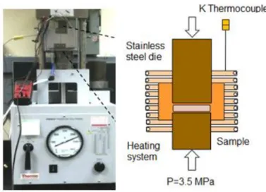
(24) 2.2 Sintering Sintering process was performed on a custom made French press-heater (Figure 5). The temperature was monitored via a high speed, high resolution data acquisition system (NIcDAQ-9174: National Instruments, Austin, TX) coupled to the equipment and measured with a K-type thermocouple. The sintering was conducted at 120, 150, 180 and 220 ºC for 3 and 5 h .These sintering temperatures were obtained based in the criteria that sintering temperature (Ts) should be conducted at Ts= (0.7-0.8) Tm [30], where Tm represent the melting point, in this case degradation and decomposition temperature. All experiments were carried out in an air atmosphere and under a constant pressure of 3.5 MPa through the entire sintering process. The temperature during sintering was measured in close proximity to the die (Figure 5). Through calibration of the equipment, it was determined that the sintering temperature can be up to 30° C lower to that measured by the thermocouple. This temperature was used to offset the collected data.. Figure 5. French press and custom designed heater system. 24.
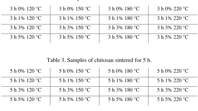
(25) 2.3 Experimental design Once the mechanical milling and sintering conditions were set up, the chitosan-CNS composites were synthesized. A nomenclature was used to identify the samples (Table 2 and. Table 3), where the first term represents the sintering time; the second term represents the reinforcer (CNS) content in the chitosan matrix expressed in weight percent (wt%), finally, the last term represents the sintering temperature. As can be observed, for each temperature and sintering time condition there exists a sample of sintered chitosan without reinforcer, these samples are denominated “control samples”, and they are used to make a comparative analysis of diverse characterization techniques with the chitosan-CNS composites and their respective sintering conditions.. Table 2. Samples of chitosan sintered for 3 h. 3 h 0% 120 °C. 3 h 0% 150 °C. 3 h 0% 180 °C. 3 h 0% 220 °C. 3 h 1% 120 °C. 3 h 1% 150 °C. 3 h 1% 180 °C. 3 h 1% 220 °C. 3 h 3% 120 °C. 3 h 3% 150 °C. 3 h 3% 180 °C. 3 h 3% 220 °C. 3 h 5% 120 °C. 3 h 5% 150 °C. 3 h 5% 180 °C. 3 h 5% 220 °C. Table 3. Samples of chitosan sintered for 5 h. 5 h 0% 120 °C. 5 h 0% 150 °C. 5 h 0% 180 °C. 5 h 0% 220 °C. 5 h 1% 120 °C. 5 h 1% 150 °C. 5 h 1% 180 °C. 5 h 1% 220 °C. 5 h 3% 120 °C. 5 h 3% 150 °C. 5 h 3% 180 °C. 5 h 3% 220 °C. 5 h 5% 120 °C. 5 h 5% 150 °C. 5 h 5% 180 °C. 5 h 5% 220 °C. 25.
(26) 2.4 Physico-chemical properties The physicochemical properties of chitosan affect its functionality and also vary depending on the source and method of obtaining the chitin, the method and the deacetylation conditions, as well as the methods and conditions for the determination of the physicochemical properties [31]. It is important to evaluate these physicochemical properties for any use that will be given to chitosan, as this will allow to know the functionality of the material regardless of its origin. The physicochemical properties of chitosan that mainly influence the functionality of chitosan are: viscosity, molecular weight and degree of deacetylation, all closely related.. 2.4.1 Determination of the deacetylation degree The degree of deacetylation is defined as the amino group content present in the polymer chain and is expressed by the percentage of free amino groups in the chitosan molecule and is closely related to its solubility [32]. The determination of the content of amino groups in the chitosan is carried out by an acidbase potentiometric titration, a method proposed by Broussignac [33], which consists in measuring the variations of the pH values to the titrator in a chitosan solution. For the potentiometric titration, 0.5 g of chitosan was dissolved with an excess of hydrochloric acid (HCl) 0.2 M to protonate the free amino group of the chitosan and then carry out a titration with sodium hydroxide (NaOH) 0.1 M until the pH of the solution is stabilized. Every 2 ml of NaOH added to the solution pH was measured with a pH potentiometer.. 26.
(27) With. the. data. obtained. a. potentiometric. curve. was. constructed.. Then a curve of titration with two inflection points is generated, whose values were determined according to the criterion of the first derivative. This difference between these points gives the ratio of the amount of acid required to protonate the amino groups of chitosan. The calculation of the concentration of the amino groups (% NH2) can be determined by the following equation [33]. % 𝑁𝐻2 =. 16.1 (𝑦−𝑥) 𝑤. 𝑓. (1). Where y is the mayor inflection point and x the lowest (both expressed as volume) f is the molarity of the NaOH solution w is the mass of the simple in grams 16.1 is a factor associated with the type of protein under study. 2.4.2 Molecular weight Chitosan is a polymer made up of repeating units of D-glucosamine, so the chain length and, therefore,. its. molecular. weight,. is. an. important. feature. of. the. molecule.. The molecular weight affects the physical and chemical properties of chitosan, as well as its functionality. Therefore the determination of the molecular weight is very important to elucidate the characteristics of the own chitosan as of its products [31]. Knowing the intrinsic viscosity the molecular weight of the sample analyzed can be analyzed, as long as the polymer obeys the Huggins equation [34] (equation 2); that is, if it presents a linear behavior between the concentration and the reduced viscosity: nsp C. = [n] + K[n]2 C. (2). The intrinsic viscosity measures the effective specific volume of an isolated polymer, reason why its determination is extrapolating to zero concentration (equation 7).. 27.
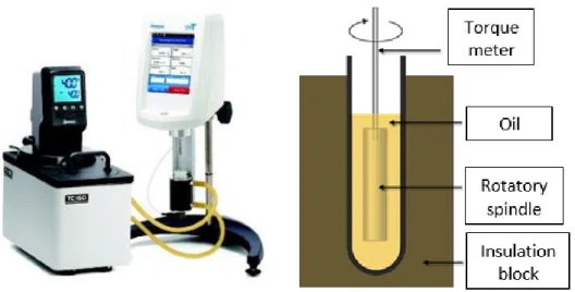
(28) The value of the intrinsic viscosity depends on the size and shape of the solute molecule, as well as its interaction with the solvent and the working temperature. For the polymer-solvent system, the Mark-Houwink equation (equation 3) [35] can be used to determine the average molecular weight of the polymer. Mv = ([n]/1.181x10−3 )1/0.93. (3). To determine the molecular weight of the chitosan, a Brookfield viscometer (Figure 6) equipped with a cooling bath was used. For the analysis 10 ml volumes of solution of chitosan at room temperature, using a number 18 spindle and a turning speed of 1000 RPM, were used. The solution of chitosan was prepared by dissolution in a mixture of acetic acid 0.1 M and sodium chloride 0.2 M. Several concentrations of chitosan were used for the analysis (2.0x10⁻³, 4.0x10⁻³, 6.0x10⁻³ and 8.0x10⁻³ g/ml).. Figure 6. Brookfield viscometer DV 2T and its main components.. 28.
(29) With the data obtained, equations 4-6 [31] were used to obtain the reduced viscosity from the viscosity measured, then the points corresponding to the reduced viscosities were plotted with respect to the concentration, and a linear regression of these were taken from the above equations; the intrinsic viscosity and then the molecular weight were determined.. 𝑛. 𝑛𝑟 = 𝑛. (4). 𝑜. Where: ɳ is the viscosity of the solution ɳo is the viscosity of the pure solvent Specific viscosity: nsp = nr − 1 nsp. Reduced viscosity: nred = (. nsp. Intrinsic viscosity: [n] = (. C. C. ). ). C→∞. (5) (6) (7). 29.
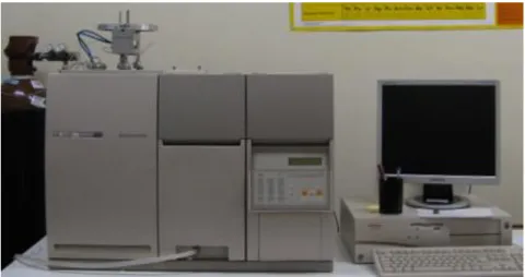
(30) 2.5 CHNS elemental analysis Carbon, hydrogen, sulphur and nitrogen contents of chitosan were determinated using CE instruments EA 110 CHNS-O Elemental Analyzer (Figure 7) .. Figure 7. CE EA 1110 CHNS Elemental Analyzer. For this analysis, a small amount of chitosan was weighed in tin capsules and then introduced into a vertical quartz reactor heated at a temperature of 1020 °C with a constant flow of helium stream. A few seconds before introducing the helium stream was enriched with high purity oxygen. The combustion gas mixture produced by the chitosan sample was driven through a tungsten oxide zone to achieve a complete quantitative oxidation followed by a reduction step in a copper zone to reduce nitrogen oxides and sulfuric anhydride to nitrogen and sulfurous anhydride. The resulting four components N2, CO2, H2O and SO2 were separated in a chromatographic column and detected by a thermos conductivity detector.. 30.
(31) The resulting signals, proportional to the amount of eluted gases, were analyzed by an automatic workstation, which provided the sample elemental composition report. Analysis was performed in a tin boat sample pan at a combustion temperature of 1150 °C and at a reduction temperature of 850 °C. Gas flow rate was 200 ml/min and 14 ml/min for helium and oxygen respectively, a whole diagram of the equipment can be seen in Figure 8.. Figure 8. Diagram of an elemental analyzer [36].. 2.6 Thermal analysis TGA was used to evaluate the thermal stability of chitosan and CNS, as well as to determine the degradation temperature of chitosan with both TGA and DSC curves. Thermogravimetric measurements were made using a DSC Auto sampler developed by TA instrument (Figure 9) with a microprocessor driven temperature control unit and a TA data station. The mass used of the samples for every sample was generally in the range of 2-3 mg.. 31.
(32) The sample pan was placed in the balance system equipment and the temperature was raised from 25 to 700 °C at a heating rate of 5 °C/min under an air atmosphere. In the case of CNS, temperature was raised from 25 to 900 °C at a heating rate of 10 °C/min under an air atmosphere. The mass of the sample pans were continuously recorded as a function of temperature.. Figure 9. DSC Auto sampler, TA instruments.. 2.7 Infrared spectroscopy Chitosan and chitosan-CNS composites were characterized by infrared spectroscopy in the region comprising from 500 to 4000 cm-1. Absorption spectra were obtained on a Fourier transform spectrophotometer Perkin Elmer (Figure 10). The powdery chitosan was mixed thoroughly with KBr and then pressed to a homogeneous disc with a thickness of 0.5 mm. The discs were scanned in the region previously mentioned to obtain FTIR spectra. No preparation of chitosan-CNS composites was done because they were already in bulk form.. 32.
(33) Figure 10. FTIR Spectrometer Perkin Elmer. An important data that can be obtained across the chitosan spectrum is the actual value of the degree of deacetylation by means of the Bruggnerotto equation (equation 8) [37] and the correlation of some vibration bands associated with the acetyl group. Appling equation 9, degree of deacetylation of chitosan was determined. 𝑁𝑎𝑐(%) = 31.92 ∗. 𝐴1318 − 12.2 𝐴1380. 𝐷𝐴(%) = 100 − 𝑁𝑎𝑐(%). (8). (9). 2.8 Raman spectroscopy For the development of this work, a confocal micro-Raman XploRA, Horiba JY (Figure 11) was used; this device is equipped with 3 lasers: 532 nm, 638 nm and 785 nm, as well as 2 optic lenses: 10x and 100x. High numerical aperture microscope objectives greatly enhance the spatial resolution and the optical collection power of the Raman instrument [30].. 33.
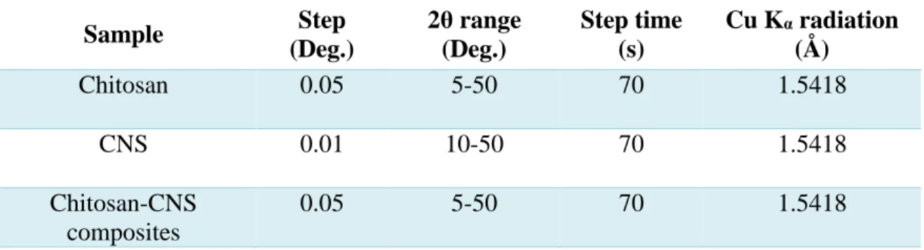
(34) Figure 11.Raman Spectrometer HORIBA XploRA. For all samples, a 638 nm diode was used to analyze the samples along with a 10x optic lens for the chitosan and 100x for the chitosan-CNS composites and CNS powders. The details of the equipment specifications are presented in Table 4. Table 4. Raman’s instrument specifications. Spectral range. 20 cm-1 to 1200 cm-1. Spectrograph:. Imaging flat field spectrometer. Detector: Microscope Confocal sampling. CCD detector Materials/clinical light microscope, Horiba Rugged confocal spatial filtering. 2.9 X-ray diffraction The technique of X-ray diffraction was used to analyses all samples. X-ray diffractograms of chitosan-CNS composites, samples of chitosan at different milling time and CNS with and without milling were obtained in order to observe the milling effect in each one of them, find. 34.
(35) their phases and calculate the crystallinity index; this last for chitosan samples and chitosanCNS composites. The crystallinity index is determined by the method of signal intensity proposed by Focher and his collaborators [38]. The crystallinity index is calculated according to the following equations: 𝐶𝐼% = [(𝐼110 − 𝐼𝑎𝑚 )/𝐼110 ] ∗ 100. (10). 𝐶𝐼% = [(𝐼020 − 𝐼𝑎𝑚 )/𝐼110 ] ∗ 100. (11). Where I110 (arbitrary units) is the maximum intensity of the (110) peak, I020 (arbitrary units) the maximum intensity of the (020) peak and Iam is the amorphous diffraction at 2θ = 12.6° (arbitrary units) [38]. For this analysis, a D8 Advance X-ray diffractometer developed by Bruker (Figure 12) was used under different conditions, which are displayed in Table 5.. Figure 12. Bruker D8 Advance diffractometer.. 35.
(36) No preparation of samples was done because chitosan and CNS were already in powder form and the chitosan-CNS composites in bulk form. Table 5. X-ray diffractometer conditions.. Chitosan. Step (Deg.) 0.05. 2θ range (Deg.) 5-50. Step time (s) 70. Cu Kα radiation (Å) 1.5418. CNS. 0.01. 10-50. 70. 1.5418. Chitosan-CNS composites. 0.05. 5-50. 70. 1.5418. Sample. 2.10 Density Densities of the chitosan-CNS composites were obtained with a Sartorius YDK01 Density Determination Kit coupled to an analytic balance (Figure 13). Here, the relationships between the mass, the volume and the density of solid bodies immersed in liquid, as described by Archimedes form a basis for the determination of the density of substances. Archimedes principle establishes that a solid immersed in a liquid is subjected to the force of buoyancy. The value of this force is the same as that of the weight of the liquid displaced by the volume of the solid [39].. Figure 13. Sartorius balance with a YDK01 density determination kit.. 36.
(37) Then, according to the previously mentioned, the beaker was placed on the pan of the balance and the sample-holding device was immersed in the liquid (in this case ethanol was used), to the same depth that the samples were immersed on it. The weighing instrument is tared. The samples was placed next to the beaker on the weighing pan. The weight of the sample in air wa (g) was determined. The samples were placed in the holding device on the stand and immersed in the liquid. The weight readout shows the displaced liquid wf (g). For every analysis temperature of the ethanol was read off to find the density ρ (fl) of the liquid (in g/cm3). Finally, the buoyancy (G) is calculated by the equation 12 [17] and the specific gravity was calculated using the equation 13. Air buoyancy is considered in equation 13 [39], as well as the additional buoyancy, caused by the immersed part of the measuring device by the geometry of the measuring device setup used in this analysis. G = wa − wf 𝜌=. 𝑤𝑎 [𝜌(𝑓𝑙)−0.0012𝑔/𝑐𝑚3 ] 0.99983 𝐺. (12) + 0.0012 𝑔/𝑐𝑚3. (13). 2.11 Porosity The porosity of the samples was determined to observe the effect of pore contraction by sintering. For this purpose, samples were cut into small pieces and dimensioned in order to obtain pieces with a uniform volume (Vc) without considering the volume of the pores. The pieces were weighed on an analytical balance to obtain the weight of the dried pieces (w1) and placed in a 10 ml beaker to be topped with ethanol of known density; then they were placed in a freezer for 40 minutes. After that the pieces were removed and the weight of the wet pieces (w2) was taken, in order to calculate the volumes of the pores (Vp) by means of the equation 15 [40]; obtaining this volume the equation 16 [40] was used to obtain the 37.
(38) volume of the skeleton of the pieces. Finally, with the data obtained, the percentage of porosity of the pieces was calculated by means of the equation 17 [40].. ρ ethanol =. w ethanol. (14). V ethanol. w2−w1. Vp = ρ ethanol. (15). Vc = Vs + Vp. (16). % porosity = (. Vc−Vs Vc. ) ∗ 100. (17). 2.12 Scanning electron microscopy The interaction of the electron beam with the sample produces different signals, as shown in Figure 14. In this work, secondary electrons and back-scattered electron were used to analyze the samples.. Figure 14. Types of interactions between electrons and sample [41]. The morphologies of chitosan samples and chitosan-CNS composites were observed in a HITACHI SU3500 (Figure 15a), operated under 15 kV in low vacuum mode (50 MPa) and a signal of back-scattered electrons. 38.
(39) The CNS were examined in a field emission JEOL JSM-7401F (Figure 15b), operated under 5 kV with a signal of secondary electrons in order to get high resolution micrographs.. Figure 15. Scanning electron microscopes. (a) HITACHI SU3500, (b) JEOL JSM-7401F.. 2.13 Transmission electron microscopy The CNS and chitosan-CNS composite morphology were observed in a transmission electron microscope HITACHI HT7700 (Figure 16) using transmitted electrons signal (bright field).. Figure 16. Transmission Electron Microscope HITACHI HT7700. CNS samples were prepared by the powder dispersion method, in which a solution was prepared by dispersing the CNS particles by means of ultrasound. Subsequently, a small amount of sample was taken with a capillary and deposited on a copper grid; then was allowed to dry the solvent. 39.
(40) In the case of the chitosan-CNS composite only a small sample was taken from the specimen to be investigated, so an extremely thin sections was obtained from the bulk material with a Power Tome Ultramicrotome (Figure 17) equipped with a glass knife. Here, a representative composite sample was cut with a diamond wafer blade in order to get a small piece similar to a pyramidal form and it was cold-mounted with epoxy resin. Once the piece was mounted, machinery was necessary to dimension the sample and place it in the ultramicrotome to get a small thin section. Finally, this thin section was deposited in a copper grid.. Figure 17. PT-PC Power Tome ultramicrotome.. 2.14 Vickers microhardness For chitosan-CNS composites microhardness analysis, the Vickers method was used on a Microdurometer LM 300 AT (Figure 18) with a load of 200 gf and dwell time of 10 s. In order to examine the chitosan-CNS composites, small pieces were cut from the composites with a diamond wafer blade and they were cold-mounted in epoxy resin. The mounted pieces were grinded with coated abrasive papers of SiC and then polished. For each sample, 6 measurements were performed in a different zone and the results were averaged.. 40.
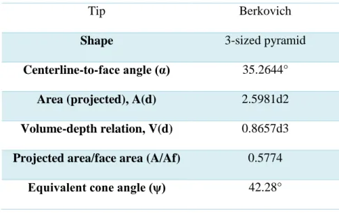
(41) Figure 18. Microdurometer LECO Series LM 300 AT.. 2.15 Nanoindentation Nanoindentation tests were performed to determine the mechanical properties at the local level of the different chitosan-CNS composites. Mechanical properties such as hardness (H) and elastic modulus (E) were evaluated in a Nano Indenter G200 (Figure 19) coupled with a DCM II head.. Figure 19. Nano Indenter G200. For this analysis, a Berkovich indenter tip was used. This tip is the most frequently used indenter tip for instrumented indentation testing to measure mechanical properties at the nanoscale. Specifications of the Berkovich tip used in this work is shown in Table 6. Table 6. Berkovich tip specifications.. 41.
(42) 35.3°. Figure 20. Nanoindenter Berkovich tip. For the sample preparation, small pieces were cut from the composites with a diamond wafer blade and directly grinded with coated abrasive papers of SiC and then polished (no resinmounting was used for this analysis). Nanoindentation tests were performed in a system with real-time data collection. The applied load was 0.2 mN and reported values are the average of 4 measurements. Table 6. Berkovich tip specifications. Tip. Berkovich. Shape. 3-sized pyramid. Centerline-to-face angle (α). 35.2644°. Area (projected), A(d). 2.5981d2. Volume-depth relation, V(d). 0.8657d3. Projected area/face area (A/Af). 0.5774. Equivalent cone angle (ψ). 42.28°. 42.
(43) 2.16 Optical microscopy An optical Axio Scope A1 polarized light microscope developed by Zeiss, equipped with ICc5 camera and AxioVision Rel. 4.8 Software for Image Acquisition and Management, was used in bright field mode (Figure 21). Chitosan-CNS composites sample previously polished (see section 2.6) were cleaned with ethanol and were examined under the optical microscope at high magnifications.. Figure 21. Axio Scope A1 microscope.. 43.
(44) CHAPTER 3 RESULTS AND DISCUSSION In this chapter the characterization results of the chitosan, CNS and chitosan-CNS composites will be presented and discussed.. 3.1 Elemental analysis Table 7 presents the elemental composition of chitosan. Comparing with the literature [42] the composition obtained through this technique fulfills the one of the theoretical elemental composition. Table 7. CHNS elemental analysis for chitosan. Sample. C%. H%. N%. S%. Theoretical. 40.68. 6.21. 7.90. 0. Chitosan. 41.30. 7.22. 7.55. Not detected. 3.2 Determination of the deacetylation degree The results of the titration are shown in Figure 22a, through this information a curve is produced with two inflection points as shown in Figure 22b, whose values were determined according to the criterion of the first derivative.. 44.
(45) a). b). Figure 22. a) Titration curve of chitosan and b) criterion of the first derivative. By means of equation 1 and the parameters shown in Table 8 for the potentiometric titration, a degree of deacetylation of 64.4% was obtained. It is important to note that chitosan is defined as chitin which has been deacetylated at 60-75% or more, at which point it becomes soluble in organic acids [43]. Table 8. Parameters obtained in the potentiometric titration. w (g) y (ml) x (ml) f (mol/L) NH2 (%) 0.5. 82. 62. 0.1. 64.4. 3.3 Determination of the molecular weight Table 9 shows the results of the measured viscosity of chitosan solutions at different concentration. Reduced viscosity was calculated applying equations 4-6 and was adjusted to the Huggins equation (equation 2).. 45.
(46) Table 9. Parameters of the viscosity tests of the chitosan sample.. Amount of Chitosan used (g). Concentration (g/ml). Viscosity of the solvent(cP). Viscosity (cP). Reduced viscosity (ml/g). 1.00. 0.002. 12.10. 20.70. 397.15. 2.00. 0.004. 12.10. 43.73. 653.52. 3.00. 0.006. 12.10. 80.89. 947.65. 4.00. 0.008. 12.10. 135.33. 1273.04. Figure 23 shows the linear regression of the reduced viscosity points as a function of the concentration for the sample of chitosan evaluated, where a linear behavior is observed.. Figure 23. Lineal regression of the viscosity points as a function of the concentration in the chitosan sample. In addition it is observed that the regression coefficient is 0.99582, which indicates that it the results complies with the Huggins equation. Applying the Mark-Honking equation (equation 3) an average molecular weight of 108,717.5 g/mol was obtained. The molecular weight. 46.
(47) calculated is within the ranges specified in the chitosan product label (50,000-190,000 g/mol).. 3.4 Thermal analysis Through the data acquisition system a heating/cooling curve for chitosan was obtained in an air atmosphere (Figure 24), where it can be identified a phase transformation at approximately 225 °C and it is attributed to the thermal degradation of the chitosan.. Figure 24. Heating/cooling curve for chitosan. Figure 24 shows TG and DTG curves for chitosan, the first thermal event is observed at 56 °C, which is attributed to the loss of water (8 wt %) weakly bound to the polymeric structure. The second thermal event is observed at 225 °C that is attributed to the degradation of the chitosan and it includes both decomposition and oxidation reactions. In the last stage, it can be seen at 287 °C a high weight loss (50 wt%) that is attributed to a depolymerization process [44].. 47.
(48) Figure 25. TG/DTG curves of chitosan. Figure 26 demonstrated trough the TG and DTG curves of CNS that it is stable to temperatures of approximately 300 °C and a weight loss (5.3 wt %) at 54 °C that is attributed to organic residue and moisture. The weight loss of the CNS during heating to 900 °C is an additional 90.5 wt % that is attributed to the oxidation of the amorphous material first, followed by oxidation of the short-order graphitic structures above 615 °C [45].. Figure 26. Thermogravimetric analysis for CNS.. 48.
(49) Figure 27 shows the main transitions of chitosan obtained through a DSC analysis in air atmosphere, in which an endothermic transition corresponding to the loss of moisture is observed at 56 ° C, followed by an exothermic transition at 287 ° C due to the decomposition process of chitosan [44].. Heat flow (mW). Exothermic. 287 °C. 56 °C. 0. 100. 200. 300. 400. 500. 600. Temperature (°C). Figure 27. DSC analysis for chitosan.. 3.5 Infrared spectroscopy Figure 28 shows the FTIR spectrum of chitosan. The main absorption bands of the chitosan functional groups are described in Table 10.. Figure 28. IR Spectrum of the chitosan. 49.
(50) Table 10. Main absorption bands for chitosan. Wave number (cm-1). Absorption bands. 3750-3000. ν(O-H) overlapped to the νs(N-H). 2920. νas(C-H). 2875. νs(C-H). 1645. ν(-C=O) secondary amide. 1574. ν(-C=O) protonated amide. 1426, 1375. δ(C-H). 1313. νs(-CH3) tertiary amide. 1261. ν(C-O-H). 1150, 1065, 1024. νas(C-O-C) and νs(C-O-C). 890. ω(C-H). Figure 29 shows the absorption spectrum in terms of absorbance, through equation 8, a value of 82.81% was obtained, which corresponds to that specified in the product label (75-85%).. 50.
(51) Absorbance (a.u.). 1310 1380. 4000 3500 3000 2500 2000 1500 1000 500 -1. Wave number (cm ). Figure 29. FTIR spectrum of chitosan (absorbance units). Figure 30 shows the FTIR spectra of chitosan after heating above its thermal degradation temperature (230 °C) for 30 min and 60 min in air atmosphere. The spectral changes are clearly seen, indicating the degradation of the polymer as a consequence of its heating. The decrease of the intensities of the band at 3280 cm-1 is attributed to dehydration due to the loss of the oxhidrile groups, at 1645 and 1580 cm-1 is observed the loss of the acetyl and amino groups and the decrease of the intensities at 2932, 2867 and all under 1420 cm-1 are attributed to depolymerization reactions [46]. All this indicates that sintering above the thermal degradation temperature causes negative effects in the synthesis of the composite, due to the loss of the main functional groups of chitosan.. 51.
(52) Figure 30. Infrared spectra of a chitosan before and after heating it 280 °C for 30 min and 60 min. In order to identify the possible interaction between chitosan and CNS, FTIR spectra form the chitosan-CNS composites were obtained. Chitosan can be linked to the CNS through the hydroxyl, amino and acetyl groups of the molecule. Figure 31 shows that the increase of intensities of O-H and N-H absorption bands (red arrows) compared with the control samples and a slight shift to the right show a possible interaction of the CNS by the oxhidrile group, as well as the increase of the intensity at 1580 cm-1 (blue arrows) corresponding to an interaction by the amino group and the increase of intensities at 2932, 2867 (black circles) and the intensity around 1313 cm-1 (black arrows) demonstrate an interaction with acetyl groups [47]. It can be seen in Figure 31b. that bonding with all main functional groups of chitosan are favored when composites are sintered for 5 h and 220 °C, as compared to those sintered at 120 ° C which are favored only by the hydroxyl and acetyl groups.. 52.
(53) a). b). Figure 31. FTIR spectra of chitosan-CNS sintered for: a) 3 h at 120 °C and b) 5 h at 220 °C. Another way of identifying possible interactions of chitosan functional groups is by the shifting of some vibration bands. Figure 32 shows that the peak at 1645 cm-1 corresponding to the secondary amine group and the small band at 1587 cm-1 assigned to N-H and amide groups of chitosan exhibit a slight shift to the right, suggesting that some amino groups were converted into amide groups and the interaction between the chitosan and CNS [47]. a). b) 5 h 0% 220 °C. 1800. 3 h 1% 120 °C. 3 h 3% 120 °C. 3 h 5% 120 °C. 1600. 1400. Wave number (cm-1). 1200. Transmittance (%). Transmittance (%). 3 h 0% 120 °C. 1800. 5 h 1% 220 °C 5 h 3% 220 °C. 5 h 5% 220 °C. 1600. 1400. 1200 -1. Wave number (cm ). Figure 32. FTIR spectra of chitosan-CNS sintered for: a) 3 h at 120 °C and b) 5 h at 220 °C.. 53.
(54) 3.6 Raman spectroscopy Figure 33 shows the main absorption Raman bands of chitosan which are described in Table 11.. Figure 33. Raman spectrum of the chitosan. Table 11. Main absorption Raman bands for chitosan. Wave number (cm-1). Absorption bands. 1654. Bond doubling -NH2. 1598. Vibrational bonding doubles N-H. 1380, 1423. Alkane C-H Bends. 1155. Antisymmetric stretches of the C-O-C bridge. 1030, 1080. Vibrations involving C-O stretching. Figure 34 shows the Raman spectra of raw and milled CNS; the two main signals correspond to the D (1366 cm-1) and G (1597 cm-1) bands that are typical of graphitic carbon [48].. 54.
(55) The D band is caused by disordered structure of graphene and it is observed in sp2 hybridized carbon systems, in the other hand, G band rises from the stretching of the C-C bond in graphitic materials, and is common to all sp2 carbon systems. Raw CNS Raman spectrum shows one second-order combinational of fullerene C60 identified at 2860 cm-1 (Ag(2)+Hg(7)) [48]. When CNS are milled, the intensity of the fullerene C60 decreased due to its fragmentation and the increasing intensity of the 2D band in the milled CNS spectrum by the formation of graphene after milling, 2D band is a secondary peak and it means the. -1. -1. -1. G (1578 cm ). Intensity (a.u.). -1. 2D (2620 cm ). D (1310 cm ). Fullerene soot. -1. D (1310 cm ). Ag(2)+Hg(7) (2860 cm ). largest intensity in single layer graphene [48].. -1. G (1578 cm ). Milled soot -1. 2D (2620 cm ). 500. 1000. 1500. 2000. 2500. 3000. -1. Raman shift (cm ). Figure 34. Raman spectra of CNS with and without milling. Figure 35Figure 36 show the Raman spectra of the control samples and the chitosan-CNS conducted at 100x and 1000x magnifications respectively. Using a 100x magnification, Raman active bands of chitosan can be identified by the vibration of the C-O stretching at 1080 and 1030 cm-1 that corresponds to the saccharide structure of chitosan, as well as the antisymmetric stretches of the C-O-C bridge at 1155 cm-1, C–H bending at approximately 1380 and 1423 cm-1 and the N–H bending found at 1598 cm-1 and corresponds to the primary amine group [49]. 55.
(56) When the analysis is conducted to at 1000x, a higher spatial resolution analysis is obtained and it allows the identification of the graphitic carbon Raman bands in the chitosan-CNS composites. Spatial resolution is determined by a combination of the laser spot size and the spacing between acquisition points on the sample and is a function of the objective magnification and the laser wavelength (higher magnification and shorter wavelengths produce smaller spot sizes) [50]. The presence of CNS in the chitosan matrix is identified by the G and D bands how are the most common bands of carbon, implying that they are located at the surface of the chitosan particles making proper interaction within in the composite. a). b) 1000X. 3 h 3% 120 °C 3 h 1% 120 °C. 3 h 0% 120 °C. 100X. 1000 1100 1200 1300 1400 1500 1600 1700 1800. 3 h 3% 150 °C. 3 h 1% 150 °C 3 h 0% 150 °C. 100X. 1000 1100 1200 1300 1400 1500 1600 1700 1800. -1. -1. Raman shift (cm ). Raman shift (cm ). c). d) 1000X. Intensity (a.u.). 3 h 3% 180 °C. 3 h 1% 180 °C. 3 h 0% 180 °C. 100X. 1000 1100 1200 1300 1400 1500 1600 1700 1800 -1. Raman shift (cm ). 1000X. 3 h 5% 220 °C. 3 h 5% 180 °C. Intensity (a.u.). 1000X. 3 h 5% 150 °C. Intensity (a.u.). Intensity (a.u.). 3 h 5% 120 °C. 3 h 3% 220 °C 3 h 1% 220 °C. 3 h 0% 220 °C. 100X. 1000 1100 1200 1300 1400 1500 1600 1700 1800 -1. Raman shift (cm ). Figure 35. Raman analysis for chitosan-CNS composites sintered for 3 h at: a) 120, b) 150, c) 180 and d) 220 °C. 56.
(57) b). a) 1000X. 5 h 3% 120 °C 5 h 1% 120 °C. 5 h 0% 120 °C. 100X. 1000 1100 1200 1300 1400 1500 1600 1700 1800. 5 h 3% 150 °C 5 h 1% 150 °C. 5 h 0% 150 °C. 100X. 1000 1100 1200 1300 1400 1500 1600 1700 1800. -1. -1. Raman shift (cm ). Raman Shift (cm ). c). d) 1000X. 5 h 5% 180 °C. 1000X 5 h 5% 220 °C. 5 h 3% 180 °C. 5 h 1% 180 °C 5 h 0% 180 °C. 100X. 1000 1100 1200 1300 1400 1500 1600 1700 1800 -1. Raman shift (cm ). Intensity (a.u.). Intensity (a.u.). 1000X. 5 h 5% 150 °C. Intensity (a.u.). Intensity (a.u.). 5 h 5% 120 °C. 5 h 3% 220 °C. 5 h 1% 220 °C. 5 h 0% 220 °C. 100X. 1000 1100 1200 1300 1400 1500 1600 1700 1800 -1. Raman shift (cm ). Figure 36. Raman analysis for chitosan-CNS composites sintered for 5 h at: a) 120, b) 150, c) 180 and d) 220 °C.. 3.7 X-ray diffraction Figure 37 shows that the X-ray diffraction pattern of chitosan consists of an amorphous and a crystalline part, reveling that chitosan is a semi-crystalline material. Chitosan has two main characteristic peaks at 2θ = 10 ° and 20 °which consist of the α-chitin and a crystal β-chitin phases, respectively [38]. α-chitin has a structure of antiparallel chains while β-chitosan has intrasheet hydrogen-bonding by parallel chains [51].. 57.
(58) Figure 37. X-ray diffractogram of chitosan. By means of the Focher equation (equation 10) it was possible to determine that the chitosan has an index of crystallinity of 58.27%. Figure 38a shows the XRD patterns of the samples of chitosan at different milling times. As can be seen in Figure 38b, as the milling time increases, the characteristic peaks of chitosan tend to widen and decrease their intensities, thus causing a reduction in their crystallinity index due to micro deformations in the crystal lattice of the material produced as a consequence high energy ball milling [52].. 58.
(59) a). b). Figure 38. a) XRD analysis of chitosan at different milling time and b) Crystallinity index analysis at different milling time. Figure 39 presents the XRD pattern of raw and milled CNS. Raw CNS show a low intensity pattern with a well-defined peak corresponding to the plane (002) and the presence of fullerene C60. XRD pattern of milled CNS showing that the plane (002) diffraction suffers an amorphization due the mechanical milling and the presence of the graphene characteristic peaks by the fragmentation of the fullerene [48].. Figure 39. X-ray diffractograms of CNS with and without milling.. 59.
(60) Figure 40 and Figure 41 show the diffraction patterns of the chitosan-CNS composites sintered for 3 h at different sintering temperatures. The α-chitin and β-chitin phases are present in each of the diffractograms as well as the characteristic peak of the deflexion of the (002) plane of amorphous graphite. When reinforcer is added to the matrix and the sintering temperature increases, the main characteristic peaks of the chitosan begin to widen and the intensities of these same ones begin to decrease, this phenomenon and with the presence of the α-chitin and β-chitin phases in the chitosan-CNS composites it is known the crystalline structure is not changed but the crystallinity index tends to decrease. One reason of the decreasing crystallinity index may be due to a kind of intermolecular reaction between CNS and chitosan, which causes that the greater the amount of reinforcer will cause the molecular chains of chitosan more difficulty to move [53]. The effects of the sintering temperature shows that the higher these conditions, the greater the mobility of the chitosan polymer chains, which indicates that there is low molecular ordering by the chains.. 60.
(61) a). b). c). d). Figure 40. XRD results of Chitosan-CNS composites sintered for 3 h at: a) 120, b) 150, c) 180 and d) 220 °C. b) a). The densities of the composites prepared by using chitosan as the matrix and hydroxyapatite, hydroxyapatite whisker, and -tricalciumphosphate as reinforcer increased and the porosities decreased with the increase in the ceramic content. The modulus of elasticity and the yield stress generally increased with the increasing ceramic content except for the chitosan/tricalciumphosphate composites. The densities and porosities of the composite structures varied in the range of 0.059-0.29 g/cm 3 and 96-88% respectively.. 61.
Figure
![Figure 2. Chemical structure of a) chitin, b) chitosan and c) chitosan partially deacetylated [7]](https://thumb-us.123doks.com/thumbv2/123dok_es/7440581.394800/14.918.323.598.499.741/figure-chemical-structure-chitin-chitosan-chitosan-partially-deacetylated.webp)
![Table 1. Some examples of chitosan reinforced applications [11].](https://thumb-us.123doks.com/thumbv2/123dok_es/7440581.394800/15.918.145.778.786.1038/table-examples-chitosan-reinforced-applications.webp)
+7
![Figure 8. Diagram of an elemental analyzer [36].](https://thumb-us.123doks.com/thumbv2/123dok_es/7440581.394800/31.918.218.701.338.696/figure-diagram-elemental-analyzer.webp)
![Figure 14. Types of interactions between electrons and sample [41].](https://thumb-us.123doks.com/thumbv2/123dok_es/7440581.394800/38.918.260.665.621.880/figure-types-interactions-electrons-sample.webp)
Documento similar