Bionomía y modelos de abundancia estacional de las especies del género Culicoides (Diptera; Ceratopogonidae) en España, con especial interés en los vectores del virus de la Lengua Azul

Texto completo

(1)TESIS DOCTORAL 2019 Bionomía y modelos de abundancia estacional de las especies del género Culicoides (Diptera; Ceratopogonidae) en España, con especial interés en los vectores del virus de la Lengua Azul. Carlos Barceló Seguí.

(2) 2.

(3) TESIS DOCTORAL 2019 Doctorado en Biotecnología Biomédica y Evolutiva Bionomía y modelos de abundancia estacional de las especies del género Culicoides (Diptera; Ceratopogonidae) en España, con especial interés en los vectores del virus de la Lengua Azul Carlos Barceló Seguí Director/a: Dr. Miguel Ángel Miranda Chueca Director/a: Dra. Bethan V. Purse Tutor/a: Dr. Carlos Juan Clar. Doctor por la Universitat de les Illes Balears 3.

(4) 4.

(5) Lista de publicaciones derivadas de la tesis: Barceló, C. & Miranda, M. A. 2017. Bionomics of livestock-associated Culicoides (biting midge) bluetongue virus vectors under laboratory conditions. Medical and Veterinary Entomology, 32(2). 216-225.. 5.

(6) 6.

(7) Dr. Miguel Ángel Miranda Chueca of the University of the Balearic Islands and Dr. Bethan V. Purse of the CEH (Center for Hydrology and Ecology). WE DECLARE:. That the thesis entitled Bionomía y modelos de abundancia estacional de las especies del género Culicoides (Diptera; Ceratopogonidae) en España, con especial interés en los vectores del virus de la Lengua Azul, presented by Carlos Barceló Seguí to obtain a doctoral degree, has been completed under our supervision and meets the requirements to opt for an International Doctorate.. For all intents and purposes, we hereby sign this document. Signatures. Dr. Miguel Ángel Miranda Chueca. Dr. Bethan V. Purse. Palma de Mallorca, 12 September 2019. 7.

(8) 8.

(9) Als meus pares. 9.

(10) 10.

(11) Agradecimientos Pareix mentida que ja faci 9 anys que em vaig ficar dins l’increïble món dels insectes. Durant tota l’etapa de la tesi he crescut com a persona, he conegut moltíssima gent i he viatjant molt, per tant, se’m fa difícil recordar-me de totes les persones a les que vull agrair. Començaré per el principi d’aquesta etapa: La primera persona que vull donar les gràcies es na Marga Miquel, es pot dir que amb ella es amb qui em vaig introduir al món dels vectors de malalties i concretament dels mosquits. Encara record aquell estiu de 2010 cercant larves de moscards a les zones inundades del Pla de Sant Jordi. Va ser tota una aventura i, la veritat, que vaig gaudir molt. A partir d’aquí, vaig sentir molta curiositat per aquest “mundillo” i vaig continuar col·laborant amb tasques del Laboratori de zoologia de la UIB. Allà vaig conèixer als que encara són els meus companys entomòlegs per excel·lència que vull anar citant un per un: En Ricardo, amb ell vaig aprendre tot sobre el món dels Culicoides i també a ser tot un Ph.D. Student professional. Ens em pegat uns bons entomoviatges a congressos on ens ho hem passat genial. Moltes gràcies per la teva saviesa. En David, un altre “veterano” i crack amb Culicoides. A veure si et treus la tesi de sobre! Na Míriam, sa crack de ses paparres. Una gran persona, afectuosa i súper amable amb la que he pogut contar-li les meves penes i problemes durant la tesi. Na Ana, un “cerebrito” que xerra, xerra i xerra i no atura. Sempre disposta a tot. Mai està aturada...te una energia infinita! Gràcies pels teus consells! No em vull deixar els altres membres del laboratori. Especialment uns dels “fundadors” del laboratori i ja retirats n’Aina Alemany i en Lluís Gállego que m’han animat i han cregut en jo des del principi, moltíssimes gràcies! També els/les altres mestres Mar, Claudia, Guillem, tots els col·laboradors que han passat per aquí com na Mariona, na Susi, na Tania...i els membres de les noves generacions com na Júlia, na Sofia, na Marian, n’Alícia, en Caye...tots han posat el seu gra d’arena! Com he comentat abans, els viatges han sigut una part important durant tota aquesta etapa. Em puc sentir afortunat d’haver assistit a tants de congressos de caire internacional i haver conegut persones de tot el món. En especial vull agrair a la Dra. Eva Veronesi, thanks for all your encouragement during my thesis period!, la Dra. Chantal de Beer i el Dr. Gert Venter your are 11.

(12) the best on Culicoides rearing!, el Dr. Luis Hernández, el Dr. Simon Carpenter, el Dr. Roger Venail i moltíssima més gent incloent Ph.D. students com en Tim, na Maria, na Laura, na Anca i un llarguíssim etcètera. Evidentment, no em deixaré els espanyols “bitxòlegs” que he conegut també viatjant: Na Sarah, na Mara, en Nacho, en Rubén, en Tomás, en David....¡gracias por toda vuestra sabiduría! Altres “mosquitòlegs” que no em vull deixar son els mes grans amics Dr. Mikel Bengoa i el senyor Raúl Luzón que ens ho hem passat genial col·laborant junts i també sortint de festa! Agrair també als meus amics personatges de tota sa vida que m’han fet “bullying” amb això de fer el doctorat, sobretot quan els hi contava que anava a “caçar bixtos”; en especial en Balaguer, en Carbo, en Bestard, en Garcis i en Paulí. No em deixaré tampoc el personal dels serveis administratius de la UIB. Moltes gràcies per fer que el nostre edifici i el nostre laboratori funcioni. Evidentment, no m’oblid del meu directors de tesi ja que sense ells no hagués arribat mai fins aquí. Gracias Dr. Miguel Ángel por ejercer este gran papel como maestro Jedi, espero que haya sido un buen padawan. Thank you so much Beth for everything, giving me the opportunity to work in the CEH and helping me during my stay in Penicuik and Wallingforf, also thanks for your patience during the modelling processes and your reviews. I also want to mention Kate, of course, many thanks for your usefull help during the models chapters of this thesis, thanks also for your patience and your friendndliness. Quasi per acabar, vull agrair tot el suport de sa meva parella, na Marina, amb la que m’he recolzat durant el darrer any d’aquest camí. Moltes gràcies per aguantar-me, t’estimo! Finalment, vull agrair a la meva família, incloent les meves dues germanes i els meus pares, els quals han tingut moltíssima paciència amb el seu fill. Esper que us sentiu orgullosos. En especial donar ses gràcies a sa meva germana Carol que m’ha dissenyat aquesta increïble portada! Gràcies sister!! La realització de part d’aquesta tesi ha sigut gràcies a les dades facilitades per la direcció general de Sanitat i Higiene Animal i Traçabilitat del Ministeri d’Agricultura, Pesca i Alimentació; així 12.

(13) com a la beca nombre 261504 del projecte EDENext, Biology and control of vector-borne infections in Europe, finançat per la Unió Europea. Gràcies als insectes!. 13.

(14) 14.

(15) Índice de contenidos Agradecimientos .......................................................................................................................... 11 Listado de figuras........................................................................................................................ 21 Listado de tablas ......................................................................................................................... 30 Listado de anexos ........................................................................................................................ 33 Listado de abreviaciones ............................................................................................................ 38 Resumen ....................................................................................................................................... 43 1. Introducción ............................................................................................................................ 55 1.1. Las enfermedades transmitidas por vectores ...................................................................... 55 1.2. El género Culicoides .......................................................................................................... 55 1.2.1. Posición Taxonómica .................................................................................................. 55 1.2.2. Distribución geográfica y hábitat ................................................................................ 56 1.2.3. Características del género Culicoides .......................................................................... 57 1.2.3.1. Morfología ............................................................................................................ 57 1.2.3.2. Ciclo biológico y comportamiento........................................................................ 66 1.2.3.3. Ciclo gonotrófico y hospedadores ........................................................................ 69 1.3. Principales patógenos transmitidos por Culicoides spp. .................................................... 70 1.3.1. Familia Reoviridae ...................................................................................................... 70 1.3.1.1. El virus de la Lengua Azul.................................................................................... 70 1.3.1.1.1. Ciclo de transmisión de la enfermedad ...................................................... 71 1.3.1.2. Peste Equina Africana (PEA)................................................................................ 72 1.3.1.3. Enfermedad Epizoótica Hemorrágica (EEH)........................................................ 73 1.3.2. Familia Bunyaviridae .................................................................................................. 73 1.3.2.1. Enfermedad de Schmallenberg (SB) ..................................................................... 73 1.3.2.2. Virus Akabane (AKAV) ....................................................................................... 73 1.3.3. Protozoos parásitos ...................................................................................................... 74 1.5. Especies implicadas en la transmisión del VLA en España ............................................... 74 1.5.1. Subgénero Avaritia Fox, 1955 ..................................................................................... 74 1.5.1.1. Complejo Imicola.................................................................................................. 74 15.

(16) 1.5.1.2. Complejo Obsoletus .............................................................................................. 75 1.5.2. Subgénero Culicoides Latreille, 1809 ......................................................................... 76 1.5.2.1. Complejo Pulicaris ................................................................................................ 76 1.6. Origen y distribución de la enfermedad en Europa y España ............................................ 78 2. Objetivos del estudio ............................................................................................................... 81 3. A Mondrian matrix of seasonal patterns of Culicoides nulliparous and parous females at different latitudes in Spain. ........................................................................................................ 83 3.1. Introduction ........................................................................................................................ 83 3.2. Material and Methods......................................................................................................... 85 3.3. Results ................................................................................................................................ 87 3.3.1. General seasonal pattern and abundance of Culicoides NF and PF in Spain between 2008 and 2010. ...................................................................................................................... 87 3.3.2. Seasonal pattern and abundance of Culicoides NF and PF from North to South axis in mainland Spain between 2008 and 2010. .............................................................................. 91 3.4. Discussion .......................................................................................................................... 95 3.4.1. General seasonal pattern and abundance of Culicoides NF and PF in Spain between 2008 and 2010. ...................................................................................................................... 95 3.4.2. Seasonal pattern and abundance of Culicoides NF and PF from North to South axis in mainland Spain. Years 2008-2010......................................................................................... 97 3.5. Conclusions ........................................................................................................................ 99 4. Environmental drivers of seasonal activity and abundance of bluetongue vector species in Spain ...................................................................................................................................... 101 4.1. Introduction ...................................................................................................................... 101 4.2. Material and methods ....................................................................................................... 105 4.2.1. Entomological data and sampling procedures ........................................................... 105 4.2.2. Models ....................................................................................................................... 106 4.2.2. Environmental parameters ......................................................................................... 108 4.2.3. Statistical methods ..................................................................................................... 111 4.3. Results .............................................................................................................................. 112 4.3.1. Comparing phenology between Culicoides taxa ....................................................... 113 4.3.2. Factors affecting the start of season .......................................................................... 116 16.

(17) 4.3.3. Factors affecting the end of season............................................................................ 116 4.3.4. Factors affecting the length of overwinter ................................................................. 117 4.4. Discussion ........................................................................................................................ 125 4.4.1. Northern species ........................................................................................................ 126 4.4.2. South-western species................................................................................................ 127 4.5. Conclusions ...................................................................................................................... 128 4.6. Annexes ............................................................................................................................ 129 5. The use of Path Analysis as a model to determine the effects of the environmental factors on the adult seasonality of Culicoides species in Spain .......................................................... 143 5.1. Introduction ...................................................................................................................... 143 5.2. Material and Methods....................................................................................................... 144 5.3. Results .............................................................................................................................. 146 5.3.1. Culicoides imicola ..................................................................................................... 146 5.3.1.1. Seasonal Start PA ................................................................................................ 146 5.3.1.2. Seasonal End PA ................................................................................................. 147 5.3.1.3. Overwintering PA ............................................................................................... 149 5.3.2. Obsoletus complex .................................................................................................... 151 5.3.2.1. Seasonal Start PA ................................................................................................ 151 5.3.2.2. Seasonal End PA ................................................................................................. 153 5.3.2.3. Overwintering PA ............................................................................................... 155 5.3.3. Culicoides newsteadi ................................................................................................. 156 5.3.3.1. Seasonal Start PA ................................................................................................ 156 5.3.3.2. Seasonal End PA ................................................................................................. 157 5.3.3.3 Overwintering PA ................................................................................................ 157 5.3.4. Culicoides pulicaris ................................................................................................... 159 5.3.4.1. Seasonal Start PA ................................................................................................ 159 5.3.4.2. Seasonal End PA ................................................................................................. 161 5.3.4.3. Overwintering PA ............................................................................................... 161 5.4. Discussion ........................................................................................................................ 167 5.5. Conclusions ...................................................................................................................... 171 5.6. Annexes ............................................................................................................................ 172 17.

(18) 6. Bionomics of livestock-associated Culicoides (biting midge) bluetongue virus vectors under laboratory conditions .................................................................................................... 187 6.1. Introduction ...................................................................................................................... 187 6.2. Material and methods ....................................................................................................... 189 6.2.1. Samplings .................................................................................................................. 189 6.2.2. Laboratory procedures ............................................................................................... 189 6.2.3. Artificial blood feeding procedures for Obsoletus complex NF ............................... 190 6.2.4. Culicoides rearing ...................................................................................................... 192 6.3. Results .............................................................................................................................. 196 6.3.1. Species composition .................................................................................................. 196 6.3.2. Oviposition ................................................................................................................ 197 6.3.3. Survival of field collected females ............................................................................ 199 6.3.4. Life-cycle and F1 adult lifespan ................................................................................ 200 6.3.5. Percentage of egg hatching, pupation success and adult emergence ......................... 202 6.3.6. Percentage of pupation per day ................................................................................. 202 6.3.7. Sex ratio ..................................................................................................................... 204 6.3.8. Artificial blood feeding for Obsoletus complex NF .................................................. 206 6.4. Discussion ........................................................................................................................ 210 6.4.1. Species composition .................................................................................................. 210 6.4.2. Oviposition ................................................................................................................ 211 6.4.3. Survival of field collected females ............................................................................ 212 6.4.4. Life-cycle and F1 adult lifespan ................................................................................ 213 6.4.5. Percentage of egg hatching, pupation success and adult emerge .............................. 214 6.4.6. Percentage of pupation per day ................................................................................. 216 6.4.7. Sex ratio ..................................................................................................................... 216 6.4.8. Artificial blood feeding for Obsoletus complex NF .................................................. 216 6.5. Conclusions ...................................................................................................................... 220 7. Study of the Obsoletus complex bionomics and other livestock associated biting midges Culicoides at different temperatures in laboratory conditions ............................................. 221 7.1. Introduction ...................................................................................................................... 221. 18.

(19) 7.2. Material and Methods....................................................................................................... 222 7.3. Results .............................................................................................................................. 225 7.3.1. Species composition and survival in sampling .......................................................... 225 7.3.2. Oviposition ................................................................................................................ 227 7.3.3. Survival of field-collected gravid females................................................................. 231 7.3.4. Life-cycle and F1 lifespan ......................................................................................... 236 7.3.5. Percentage of egg hatching, pupation success and adult emergence ......................... 237 7.3.6. Pupation ..................................................................................................................... 240 7.3.7. Larvae growing .......................................................................................................... 243 7.3.8. Sex ratio ..................................................................................................................... 244 7.4. Discussion ........................................................................................................................ 244 7.4.1. Species composition and survival in sampling .......................................................... 244 7.4.2. Oviposition ................................................................................................................ 245 7.4.3. Survival of field-collected gravid females................................................................. 247 7.4.4. Life-cycle and F1 adult lifespan ................................................................................ 248 7.4.5. Percentage of egg hatching, pupation success and adult emergence ......................... 249 7.4.6. Pupation ..................................................................................................................... 251 7.4.7. Larvae growth ............................................................................................................ 251 7.4.8. Sex ratio ..................................................................................................................... 251 7.5. Conclusions ...................................................................................................................... 252 8. Recapitulación ....................................................................................................................... 255 9. Conclusions ............................................................................................................................ 261 10. Referencias bibliográficas .................................................................................................. 263. 19.

(20) 20.

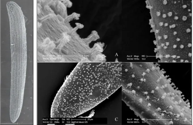
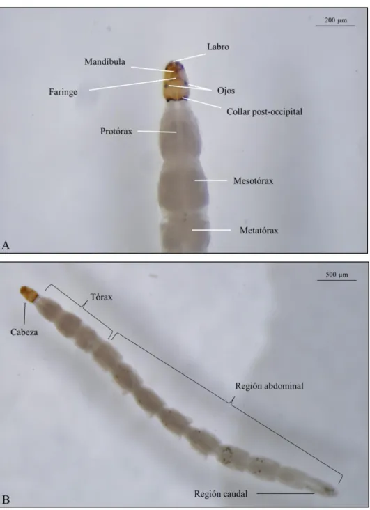
(21) Listado de figuras Figura 1. Fotografías con microscopio electrónico de barrido. Izquierda: Vista lateral de un huevo de Culicoides circumscriptus Kieffer. Escala 50 μg. Fuente: Day et al. (1997). Derecha: Detalle de la ornamentación de la superficie del huevo de C. sonorensis. Distintas escalas. Fuente: Abubekerov (2014) y Abubekerov & Mullens (2017). Figura 2. Fotografías realizadas con lupa binocular del detalle de la región cefálica y tórax de una larva L4 de Culicoides paolae Boorman (A). Detalle del cuerpo entero de la larva donde se observan los segmentos abdominales (B). Fuente: C. Barceló. Figura 3. Detalle de la cabeza de una larva L4 de Culicoides obsoletus (Meigen) realizada con microscopio electrónico de barrido. Vista ventral (A) y vista latero-ventral (B). Fuente: C. Barceló. Figura 4. Detalle de la región caudal de una larva L4 de C. obsoletus realizada con microscopio electrónico de barrido. Vista dorsal (A) y vista ventral (B). Fuente: C. Barceló. Figura 5. Vista dorsal de una pupa de C. circumscriptus (A) y vista ventral de una pupa de C. paolae (B) realizadas con microscopio electrónico de barrido. Fuente: C. Barceló. Figura 6. Detalle de la región cefálica de la pupa donde se aprecian los cornetes respiratorios y la localización de los poros realizada con microscopio electrónico de barrido. Vista dorsal de C. circumscriptus (A) y vista ventral de C. paolae (B). Fuente: C. Barceló. Figura 7. Detalle del lóbulo genital de una pupa donde se aprecia el dimorfismo sexual. Hembra de C. circumscriptus (A) y macho de C. paolae (B). Fuente: C. Barceló. Figura 8. Aspecto general de un Culicoides adulto, en este caso, C. impunctatus. Se puede apreciar el patrón de manchas alares característico de esta especie. (Diseño de Carim Nahaboo). Figura 9. Macho de C. obsoletus realizada con estereomicroscopio. Se pueden observar las antenas plumosas y la genitalia. Fuente: C. Barceló. Figura 10. Ejemplo de los 4 estadios larvarios (L1-L4) de C. sonorensis donde se observa la diferencia de tamaño y de su cápsula cefálica. Fuente: Abubekerov (2014) y Abubekerov & Mullens (2017). 21.

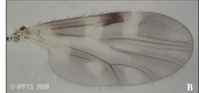
(22) Figura 11. Pareja de C. obsoletus apareándose capturada en un enjambre mediante manga entomológica (A) y detalle de la genitalia durante la cópula (B). Fuente: González et al. (2017). Figura 12. Estados gonotróficos de hembras de Culicoides realizadas con estereomicroscopio. Hembra nulípara de C. obsoletus (A), grávida de C. obsoletus (B), para de C. obsoletus (C) y alimentada de sangre de C. imicola (D). Fuente: C. Barceló. Figura 13. Esquema del ciclo de transmisión del VLA. Fuente: Purse et al. (2005) Figura 14. Patrón de manchas alares de C. imicola (A) y C. obsoletus (B). Fuente: Mathieu et al. (2012). Figura 15. Detalle del patrón de manchas alares de dos especies del Complejo Pulicaris presentes en España donde también se comparan las dos especies crípticas de C. pulicaris (arriba). Detalle del patrón de manchas alares de las tres especies crípticas del Complejo Newsteadi (abajo). Fuente: Pagès (2009). Figura 16. Mapa de las zonas de restricción de animales debido al VLA en Europa (actualizado a enero de 2019) donde se representan los diferentes serotipos circulando en los países y regiones europeas. Fuente: Comisión Europea (2018). Figure 17. Location of the provinces included in the analysis of maximum monthly catches of nulliparous females (NF) and parous females (PF) of Obsoletus complex, C. pulicaris, C. imicola and C. newsteadi from North to South of mainland Spain. Navarra (Na.), Zaragoza (Za.), Guadalajara (Gu.), Toledo (To), Ciudad Real (C.R.), Córdoba (Có.) and Cádiz (Cá.). In brackets: number of selected locations / number sampling stations. Figure 18. Mondrian matrix of the weekly maximum catches of nulliparous (NF) and parous females (PF) from 2008 to 2010 in mainland Spain (colour coded) for the species Obsoletus complex, C. pulicaris, C. imicola and C. newsteadi. Light green= 0 individuals, dark green= 1-4 individuals, yellow= 5-9, orange= 10-199, red= 200-499, dark red= 500-999, purple= 10002999, blue= 3000-5000. Letters indicate significant differences between species among seasons being (A): Significant differences respect the other species (2-tailed K-S tests, P<0.05), (B): Significant differences respect to C. newsteadi and C. pulicaris (2-tailed K-S tests, P<0.05), (C): Significant differences respect to C. pulicaris (2-tailed K-S tests, P<0.05). 22.

(23) Figure 19. Mondrian matrix of the monthly maximum catches of nulliparous (NF) and parous females (PF) from 2008 to 2010 between the Northern province (Navarra) and the Southern one (Cádiz) (colour coded) for the species Obsoletus complex (above) and C. pulicaris (bellow). Green= 0 individuals, dark green= 1-4, yellow= 5-9, orange= 10-39, red= 40-99, purple= 100499, blue= 500-1000. Letters indicate significant differences among provinces being (a): significant differences respect to the other six provinces (2-talied K-S tests, P<0.05), (b): significant differences respect to the Southern provinces (2-tailed K-S test, P<0.05). Figure 20. Mondrian matrix of the monthly maximum catches of nulliparous (NF) and parous females (PF) from 2008 to 2010 between the Northern province (Navarra) and the Southern one (Cádiz) (colour coded) for the species C. imicola (above) and C. newsteadi (bellow). Green= 0 individuals, dark green= 1-4, yellow= 5-9, orange= 10-39, red= 40-99, purple= 100-499, blue= 500-1000. Letters indicate significant differences among provinces being (a): significant differences respect to the other six provinces (2-talied K-S tests, P<0.05), (c): significant differences respect to Cádiz province (2-talied K-S tests, P<0.05). Figure 21. Map with the location of sampling points during the National surveillance program from 2005 to 2010. Figure 22. Differences between species in the timing of the start (A) and end (B) of seasonal activity (weeks of the year), and length of overwinter period (C; days) derived from Spain National Surveillance Program data during 2005 to 2010. Box plots show the median (central line), box denotes 25th and 75th percentiles, error bars represent 10th and 90th percentiles, and dots are points outside the 10th and 90th percentiles. Data are shown for C. imicola (IMI, N= 57), C. newsteadi (NEW, N= 58), Obsoletus complex species (OBS, N= 84), and C. pulicaris (PUL, N= 40). Figure 23. Structural equation model diagram for how the seasonal metrics of different Culicoides species are affected directly by environmental variables and indirectly via annual Culicoides abundance of females for sites in Spain. Figure 24. Path diagrams for models for the timing of the start of the season of C. imicola nulliparous females (NF). Thick solid lines represent strong evidence for an effect (95 % credible interval does not overlap zero), while dotted lines represent no effect. Plus sign indicates a 23.

(24) positive relationship between the timing of the start of the season and the predictor variable. Numbers on the unbroken arrows represent the posterior mean and credible interval and percentage of posterior values that are above or below zero. Figure 25. Path diagrams for models for the timing of the end of the season of C. imicola. (A): nulliparous females (NF); (B): parous females (PF). Thick solid lines represent strong evidence for an effect (95 % credible interval does not overlap zero), while thin grey lines represent weak evidence for an effect (90 % credible interval does not overlap zero). Dotted lines represent no effect. Plus sign indicates a positive relationship between the timing of the end of the season and the predictor variable, while minus sign indicates negative relationship. Numbers on the unbroken arrows represent the posterior mean and credible interval and percentage of posterior values that are above or below zero. Figure 26. Path diagrams for models for the timing of the length of overwinter period of C. imicola. (A): nulliparous females (NF); (B): parous females (PF).Thick solid lines represent strong evidence for an effect (95 % credible interval does not overlap zero), while thin grey lines represent weak evidence for an effect (90 % credible interval does not overlap zero). Dotted lines represent no effect. Plus sign indicates a positive relationship between the timing of the length of overwinter and the predictor variable, while minus sign indicates negative relationship. Numbers on the unbroken arrows represent the posterior mean and credible interval and percentage of posterior values that are above or below zero. Figure 27. Path diagrams for models for the timing of the start of the season of Obsoletus complex. (A): nulliparous females (NF); (B): parous females (PF). Thick solid lines represent strong evidence for an effect (95 % credible interval does not overlap zero), while thin grey lines represent weak evidence for an effect (90 % credible does not overlap zero). Dotted lines represent no effect. Plus sign indicates a positive relationship between the timing of the start of season and the predictor variable, while minus sign indicates negative relationship. Numbers on the unbroken arrows represent the posterior mean and credible interval and percentage of posterior values that are above or below zero. Figure 28. Path diagrams for models for the timing of the end of the season of Obsoletus complex. (A): nulliparous females (NF); (B): parous females (PF). Thick solid lines represent 24.

(25) strong evidence for an effect (95 % credible interval does not overlap zero), while thin grey lines represent weak evidence for an effect (90 % credible interval does not overlap zero). Dotted lines represent no effect. Plus sign indicates a positive relationship between the timing of the end of season and the predictor variable, while minus sign indicates negative relationship. Numbers on the unbroken arrows represent the posterior mean and credible interval and percentage of posterior values that are above or below zero. Figure 29. Path diagrams for models for the timing of the length of overwinter period of Obsoletus complex nulliparous females (NF). Thick solid lines represent strong evidence for an effect (95 % credible interval does not overlap zero), while dotted lines represent no effect. Plus sign indicates a positive relationship between the timing of the length of overwinter and the predictor variable. Numbers on the unbroken arrows represent the posterior mean and credible interval and percentage of posterior values that are above or below zero. Figure 30. Path diagrams for models for the timing of the start of the season of C. newsteadi parous females (PF). Thick solid lines represent strong evidence for an effect (95 % credible interval does not overlap zero), while thin grey lines represent weak evidence for an effect (90 % credible interval does not overlap zero). Dotted lines represent no effect. Plus sign indicates a positive relationship between the timing of the start of the season and the predictor variable, while minus sign indicates negative relationship. Numbers on the unbroken arrows represent the posterior mean and credible interval and percentage of posterior values that are above or below zero. Figure 31. Path diagrams for models for the timing of the length of overwinter period of C. newsteadi. (A): nulliparous females (NF); (B): parous females (PF). Thick solid lines represent strong evidence for an effect (95 % credible interval does not overlap zero), while thin grey lines represent weak evidence for an effect (90 % credible interval does not overlap zero). Dotted lines represent no effect. Plus sign indicates a positive relationship between the timing of the length of overwinter and the predictor variable, while minus sign indicates negative relationship. Numbers on the unbroken arrows represent the posterior mean and credible interval and percentage of posterior values that are above or below zero.. 25.

(26) Figure 32. Path diagrams for models for the timing of the start of season of C. pulicaris. (A): nulliparous females (NF); (B): parous females (PF). Thick solid lines represent strong evidence for an effect (95 % credible interval does not overlap zero), while dotted lines represent no effect. Minus sign indicates a negative relationship between the timing of the start of season and the predictor variable. Numbers on the unbroken arrows represent the posterior mean and credible interval and percentage of posterior values that are below zero. Figure 33. Path diagrams for models for the timing of the length of overwinter period of C. pulicaris. (A): nulliparous females (NF); (B): parous females (PF). Thick solid lines represent strong evidence for an effect (95 % credible interval does not overlap zero), while thin grey lines represent weak evidence for an effect (90 % credible interval does not overlap zero). Dotted lines represent no effect. Plus sign indicates a positive relationship between the timing of the length of overwinter and the predictor variable, while minus sign indicates negative relationship. Numbers on the unbroken arrows represent the posterior mean and credible interval and percentage of posterior values that are above or below zero. Figure 34. Cardboard box with 5 cm plastic Petri dish at the bottom provided with moistened cotton wool and filter paper as substrate for oviposition of Culicoides females. Figure 35. Glass beads in 250 ml containers used for defibrinating blood (A). Containers filled with the glass beads and bovine blood (B). Figure 36. Parafilm® artificial membrane attached to the Hemotek© arm (A). Hemotek© arm set on top of the cardboard box with the C. obsoletus nulliparous females inside (B). Figure 37. Example of oviposited eggs on the 5 cm plastic Petri dish at the bottom of cardboard boxes provided with moistened cotton wool and filter paper. Figure 38. Oviposited eggs transferred to a to 100 mm Petri dishes with 10 ml of 2% European Bacteriological Agar gel medium. Figure 39. First instar larvae just emerged from the egg on the agar gel medium. Hatched eggs and its opercles are also observed.. 26.

(27) Figure 40. Fourth instar Culicoides larvae feeding upon nematode (pointed with a white arrow) in agar gel medium. Figure 41. Pupae on the agar gel medium of the Petri dish (A). Pupae transferred to the Petri dish of the cardboard boxes for adult emergence (B). Figure 42. Emerged Culicoides individuals observed through the cardboard box mesh (A). Culicoides individual emerging from the pupa (B). Figure 43. Percentages of different gonotrophic stages among the total Culicoides individuals collected from field. W/A (Without Abdomen): Individuals that had lost their abdomens such that gonotrophic stage was impossible to determine. Figure 44. Percentages species composition from the total Culicoides individuals (females and males) collected from field. Figure 45. Percentage of field-collected gravid Culicoides females that oviposited. (#): Sample size. Figure 46. Average (Av) time ± S. D. (Standard Deviation) to oviposit of field-collected, gravid Culicoides females. (*): Based on eggs and larvae of a single individual of C. imicola. Figure 47. Average lifespan ± S. D. of field-collected, gravid Culicoides females and survival after oviposition. (*): C. imicola individual died immediately after oviposition. Figure 48. Percentage of sub-adult and adult stages duration, estimated from Culicoides field gravid females progeny. (#): Sample size. Figure 49. Percentage of larvae that pupated daily, estimated from the progeny of each field collected, gravid Culicoides female. Figure 50. Average percentage ± S. D. of adult males and females emerged in the laboratory by Culicoides species emerged in the laboratory (*): C. imicola progeny are from only one fieldcollected gravid female.. 27.

(28) Figure 51. Percentage of oviposition of field-collected Obsoletus complex nulliparous females fed through artificial membrane versus oviposition of field-collected, gravid Obsoletus complex females. (#): Sample size. Figure 52. Average ± S. D. lifespan of field-collected C. obsoletus nulliparous females fed through artificial membrane after feeding versus average lifespan of field-collected, gravid C. obsoletus females and survival after oviposition. Figure 53. Average time ± S. D. to oviposit, to egg hatch, larval period and time to adult emergence of field-collected C. obsoletus nulliparous females fed through artificial membrane versus field-collected, gravid C. obsoletus females. Figure 54. Percentage of F1 males and females emerged in the laboratory from C. obsoletus artificially fed and C. obsoletus field gravid females. Figure 55. Average number ± S. D. of eggs, pupae and adults obtained from field-collected C. obsoletus nulliparous females fed through artificial membrane versus field-collected, gravid C. obsoletus females. Figure 56. Location of the two sampled livestock farms in Majorca Island. Figure 57. Percentag of field gravid females from Can Cosme (A) and Son Ajaume (B) that oviposited at different temperatures. (#): Sample size. (*): The species only oviposited at 18ºC. (x): The species only oviposited at 30ºC. (†): The individuals at 25º did not survive. Figure 58. Average time to oviposit (in days) ± S. D. of field gravid females from Can Cosme (A) and Son Ajaume (B) at different temperatures. Only species with data from the three temperatures are represented. (c): Significant differences with respect to the 30ºC (K-S, P<0.05). In brackets: Sample size. Figure 59. Average number of eggs laid ± S. D. of the field gravid females from Can Cosme (A) and Son Ajaume (B) at different temperatures. (#): Sample size. Figure 60. Lifespan of field gravid females from Can Cosme (A) and Son Ajaume (B) at different temperatures and the lifespan after oviposition in Can Cosme (C) and Son Ajaume (D). Only species with data from the three tested temperatures are represented. In brackets: Sample 28.

(29) size. (a): Significant differences with respect to the other temperatures (2-tailed K-S test, P<0.05). (b): Significant differences with respect to 25ºC (2-tailed K-S test, P<0.05). (c): Significant differences with respect to 30ºC (2-tailed K-S test, P<0.05). Figure 61. Average of sub-adult stages duration in days and F1 adult survival of each Culicoides species from Can Cosme (A) and Son Ajaume (B). (#): Sample size. Figure 62. Average percentage ± S. D. of egg hatching obtained from Culicoides field gravid females in Can Cosme (A) and Son Ajaume (B) at different temperatures. (#): Sample size. Figure 63. Average percentage ± S. D. of pupation. of F1 Culicoides species from Can Cosme (A) and Son Ajaume (B). (#): Sample size. Figure 64. Average percentage ± S. D. of adult emergence of F1 Culicoides species from Can Cosme (A) and Son Ajaume (B). (b): Significant differences between both temperatures (T-test, P<0.05). (#): Sample size. Figure 65. Number of daily L4 larvae of C. obsoletus that pupated from Can Cosme at 18ºC and 25ºC. Figure 66. Number of daily L4 larvae of C. circumscriptus that pupated from Can Cosme (A) and Son Ajaume (B) at 18ºC, 25ºC and 30ºC. Figure 67. Number of daily L4 larvae of C. paolae that pupated from Son Ajaume at 30ºC. Figure 68. Average length of larval growth (in mm per day) ± S. D. of each species from Can Cosme (A) and Son Ajaume (B) at different temperatures in laboratory conditions. (a): Significant differences of 18ºC with respect the other temperatures. (b): Significant differences between 18ºC and 25ºC (K-S test P<0.05). (#): Sample size. Figure 69. Percentage of total adults males and females for each species that emerged at different temperatures) in the laboratory from Can Cosme (A) and Son Ajaume (B). (#): Sample size.. 29.

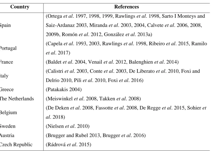
(30) Listado de tablas Table 1. List of countries with National Surveillance programs for Culicoides vector species in Europe with references. Table 2. Percentage of the annual total maximum catches of nulliparous females (NF) and parous females (PF) for each Culicoides species that were captured in each season during the years 2008 and 2010 in mainland Spain. Table 3. Summary of vector species incriminated as vectors in Spain and their distribution. Species and virus strains from other continents are not included. Table 4. Number of total data points and data points after species abundance thresholds had been applied. For start and end of season, thresholds were as follows: Obsoletus complex: >1 females / trap catch, for C. newsteadi and C. pulicaris: >5 females / trap catch and for C. imicola >20 females / trap catch. For length of overwinter period, thresholds were: Obsoletus complex, C. newsteadi and C. pulicaris: >1 females / trap catch and for C. imicola >20 females / trap catch. N: number of samples. Table 5. Environmental variables included as potential predictors of patterns in Culicoides phenology in Spain (timing of start and end of season, and length of overwinter (OW)) extracted for each of the trapping site by year combinations. Table 6. Total and mean number of Culicoides caught by site and year used in analysis with thresholds applied for Obsoletus complex: >1 females / trap catch, for C. newsteadi and C. pulicaris: >5 females / trap catch and for C. imicola >20 females / trap catch. N: number of samples. (*): No catches in 2005. Table 7. Estimated posterior mean values and credible intervals when more than 95% of posterior values are above or below zero for the coefficients for environmental fixed variables of the best Obsoletus complex model within the three different seasonal metrics. (*): indicate significance for environmental variables. ρ= Spearman’s rho. Appearance: percentage of the top models in which the significant variables appear..

(31) Table 8. Estimated posterior mean values and credible intervals when more than 95% of posterior values are above or below zero for the coefficients for environmental fixed variables of the best C. imicola model within the three different seasonal metrics. ρ= Spearman’s rho. Appearance: percentage of the top models in which the significant variables appear. Table 9. Estimated posterior mean values and credible intervals when more than 95% of posterior values are above or below zero for the coefficients for environmental fixed variables of the best C. newsteadi model within the three different seasonal metrics. (*): indicate significance for environmental variables. ρ= Spearman’s rho. Appearance: percentage of the top models in which the significant variables appear. Table 10. Estimated posterior mean values and credible intervals when more than 95% of posterior values are above or below zero for the coefficients for environmental fixed variables of the best C. pulicaris model within the three different seasonal metrics. (*): indicate significance for environmental variables. ρ= Spearman’s rho. Appearance: percentage of the top models in which the significant variables appear. Table 11. Summary of the significant environmental parameters for each species and seasonal metric. Appearance: Percentage of seasonal metrics in which the variable was significant across all the species. Elev. Elevation; AgFor: Agro-forestry areas; SchVeg: Schlerophyllous vegetation; DDwin/aut/spr: Accumulated degree days over 10ºC in winter, autumn and spring; Paut/win: Precipitation in autumn and spring; Phapr/sep: Photoperiod in April and September; sum fem: Culicoides females abundance. (+): positive effect, (-): negative effect. Table 12. Summary of the significant environmental parameters for Start of the season models of each species. NF: Nulliparous females, PF: Parous females. Light grey: Variables included in the best model, dark grey: variable with weak effect (90% of credible interval did not include zero), black: Variable with strong effect (95% of credible interval did not include zero). (+): Positive effect, (-): Negative effect, (A): Indirect effect via Culicoides females abundance. Table 13. Summary of the significant environmental parameters for End of the season models of each species. NF: Nulliparous females, PF: Parous females. Light grey: Variables included in the best model, dark grey: Variable with weak effect (90% of credible interval did not include zero),. 31.

(32) black: Variable with strong effect (95% of credible interval did not include zero). (+): Positive effect, (-): Negative effect, (A): Effect on the Culicoides females abundance. Table 14. Summary of the significant environmental parameters for Length of overwinter of each species. NF: Nulliparous females, PF: Parous females. Light grey: Variables included in the best model, dark grey: Variable with weak effect (90% of credible interval did not include zero), black: Variable with strong effect (95% of credible interval did not include zero). (+): Positive effect, (-): Negative effect, (A): Effect on the Culicoides females abundance. Table 15. Range in size of egg batch for various Culicoides species. SA: South Africa. Table 16. Average duration (days) ± S.D. of the life stages (egg, larva, pupa, F1 adults) of Culicoides species reared under laboratory conditions. Table 17. Percentages of egg hatching, larvae pupation and adults emerged for individuals of each Culicoides species obtained from field gravid females ± S. D. Table 18. Summarize of reproductive potential across the parameters measured from each Culicoides species. Positive parameters: Parameters that increase the suitability of the species to laboratory conditions. Negative parameters: Parameters that decrease the suitability of the species to laboratory conditions. Sex ratio= 1- (% females/% males). Total values of the last column are the results of the following equation: (positive parameters-negative parameters). Table 19. Percentage of egg hatching, larvae pupation and F1 adults emerged from C. obsoletus individuals artificially fed and C. obsoletus field gravid females ± S. D. Table 20. Species and number of animals in the sampled farms Can Cosme and Son Ajaume. Table 21. Number of alive gravid and total Culicoides species collected in both livestock farms with sampling survival rates. In brackets: total individuals. GF: gravid females. Table 22. Time to oviposit of field gravid females from Can Cosme (A) and Son Ajaume (B) at different temperatures. In brackets: Sample size. (c): Significant differences with respect to 30ºC (K-S, P<0.05).. 32.

(33) Table 23. Lifespan of field gravid females from Can Cosme (A) and Son Ajaume (B) at different temperatures. In brackets: Sample size. (T): Total average. (a): Significant differences with respect to the other temperatures (2-tailed K-S test, P<0.05). (b): Significant differences with respect to 25ºC (2-tailed K-S test, P<0.05). (c): Significant differences with respect to 30ºC (2tailed K-S test, P<0.05). Table 24. Lifespan after oviposition of field gravid females from Can Cosme (A) and Son Ajaume (B) at different temperatures. In brackets: Sample size. (T): Total average. (*): The species only oviposit at 18ºC. (#): The species only oviposit at 30ºC.. Listado de anexos Annex 2. Top 10 models for Obsoletus complex start of the season (best model in grey). a= intercept. pD: Effective number of parameters in each model. DIC: Deviance information criterion. ∆ DIC: Difference in DIC between each model and the best model. n= Number of observations with > 1 individuals per trap. Annex 3. Top 10 models for C. imicola start of the season (best model in grey). a= intercept. pD: Effective number of parameters in each model. DIC: Deviance information criterion. ∆ DIC: Difference in DIC between each model and the best model. n= Number of observations with > 20 individuals per trap. Annex 4. Top 10 models for C. newsteadi start of the season (best model in grey). a= intercept. pD: Effective number of parameters in each model. DIC: Deviance information criterion. ∆ DIC: Difference in DIC between each model and the best model. n= Number of observations with > 5 individuals per trap. Annex 5. Top 10 models for C. pulicaris start of the season (best model in grey). a= intercept. pD: Effective number of parameters in each model. DIC: Deviance information criterion. ∆ DIC: Difference in DIC between each model and the best model. n= Number of observations with > 1 individuals per trap. Annex 6. Top 10 models for Obsoletus complex end of the season (best model in grey). a= intercept. pD: Effective number of parameters in each model. DIC: Deviance information. 33.

(34) criterion. ∆ DIC: Difference in DIC between each model and the best model. n= Number of observations with > 1 individuals per trap. Annex 7. Top 10 models for C. imicola end of the season (best model in grey). a= intercept. pD: Effective number of parameters in each model. DIC: Deviance information criterion. ∆ DIC: Difference in DIC between each model and the best model. n= Number of observations with > 20 individuals per trap. Annex 8. Top 10 models for C. newsteadi end of the season (best model in grey). a= intercept. pD: Effective number of parameters in each model. DIC: Deviance information criterion. ∆ DIC: Difference in DIC between each model and the best model. n= Number of observations with > 5 individuals per trap. Annex 9. Top 10 models for C. pulicaris end of the season (best model in grey). a= intercept. pD: Effective number of parameters in each model. DIC: Deviance information criterion. ∆ DIC: Difference in DIC between each model and the best model. n= Number of observations with > 1 individuals per trap. Annex 10. Top 10 models for Obsoletus complex overwinter (OW) season (best model in grey). a= intercept. pD: Effective number of parameters in each model. DIC: Deviance information criterion. ∆ DIC: Difference in DIC between each model and the best model. n= Number of observations with > 1 individuals per trap. Annex 11. Top 10 models for C. imicola overwinter (OW) season (best model in grey). a= intercept. pD: Effective number of parameters in each model. DIC: Deviance information criterion. ∆ DIC: Difference in DIC between each model and the best model. n= Number of observations with > 20 individuals per trap. Annex 12. Top 10 models for C. newsteadi overwinter (OW) season (best model in grey). a= intercept. pD: Effective number of parameters in each model. DIC: Deviance information criterion. ∆ DIC: Difference in DIC between each model and the best model. n= Number of observations with > 5 individuals per trap. Annex 13. Top 10 models for C. pulicaris overwinter (OW) season (best model in grey). a= intercept. pD: Effective number of parameters in each model. DIC: Deviance information 34.

(35) criterion. ∆ DIC: Difference in DIC between each model and the best model. n= Number of observations with > 1 individuals per trap. Annex 14. Best Start of the season models for NF and PF of each Culicoides species. pD: Effective number of parameters in each model. DIC: Deviance Information Criterion. N: Number of samples. Annex 15. Best End of the season models for NF and PF of each Culicoides species. pD: Effective number of parameters in each model. DIC: Deviance information criterion. N: Number of samples. Annex 16. Best Length of Overwinter models for NF and PF of each Culicoides species. pD: Effective number of parameters in each model. DIC: Deviance information criterion. OW: Days overwintering. N: Number of samples. Annex 17. Top 3 Start of the season models for C. imicola NF and PF (best model in grey). a: Intercept. pD: Effective number of parameters in each model. DIC: Deviance information criterion. ∆ DIC: Difference with the best model. n= Number of samples with > 20 individuals per trap. N pred.: Number of predictors used in the model. Annex 18. Top 3 Start of the season models for Obsoletus complex NF and PF (best model in grey). a: Intercept. pD: Effective number of parameters in each model. DIC: Deviance information criterion. ∆ DIC: Difference with the best model. n= Number of samples with > 1 individuals per trap. N pred.: Number of predictors used in the model. Annex 19. Top 3 Start of the season models for C. newsteadi NF and PF (best model in grey). a: Intercept. pD: Effective number of parameters in each model. DIC: Deviance information criterion. ∆ DIC: Difference with the best model. n= Number of samples with > 5 individuals per trap. N pred.: Number of predictors used in the model. Annex 20. Top 3 Start of the season models for C. pulicaris NF and PF (best model in grey). a: Intercept. pD: Effective number of parameters in each model. DIC: Deviance information criterion. ∆ DIC: Difference with the best model. n= Number of samples with > 5 individuals per trap. N pred.: Number of predictors used in the model.. 35.

(36) Annex 21. Top 3 End of the season models for C. imicola NF and PF (best model in grey). a: Intercept. pD: Effective number of parameters in each model. DIC: Deviance information criterion. ∆ DIC: Difference with the best model. n= Number of samples with > 5 individuals per trap. N pred.: Number of predictors used in the model. Annex 22. Top 3 End of the season models for Obsoletus complex NF and PF (best model in grey). a: Intercept. pD: Effective number of parameters in each model. DIC: Deviance information criterion. ∆ DIC: Difference with the best model. n= Number of samples with > 5 individuals per trap. N pred.: Number of predictors used in the model. Annex 23. Top 3 End of the season models for C. newsteadi NF and PF (best model in grey). a: Intercept. pD: Effective number of parameters in each model. DIC: Deviance information criterion. ∆ DIC: Difference with the best model. n= Number of samples with > 5 individuals per trap. N pred.: Number of predictors used in the model. Annex 24. Top 3 End of the season models for C. pulicaris NF and PF (best model in grey). a: Intercept. pD: Effective number of parameters in each model. DIC: Deviance information criterion. ∆ DIC: Difference with the best model. n= Number of samples with > 5 individuals per trap. N pred.: Number of predictors used in the model. Annex 25. Top 3 Length of Overwinter models for C. imicola NF and PF (best model in grey). a: Intercept. pD: Effective number of parameters in each model. DIC: Deviance information criterion. ∆ DIC: Difference with the best model. n= Number of o samples with > 5 individuals per trap. N pred.: Number of predictors used in the model. Annex 26. Top 3 Length of Overwinter models for Obsoletus complex NF and PF (best model in grey). a: Intercept. pD: Effective number of parameters in each model. DIC: Deviance information criterion. ∆ DIC: Difference with the best model. n= Number of samples with > 5 individuals per trap. N pred.: Number of predictors used in the model. Annex 27. Top 3 Length of Overwinter models for C. newsteadi NF and PF (best model in grey). a: Intercept. pD: Effective number of parameters in each model. DIC: Deviance information criterion. ∆ DIC: Difference with the best model. n= Number of samples with > 5 individuals per trap. N pred.: Number of predictors used in the model. 36.

(37) Annex 28. Top 3 Length of Overwinter models for C. pulicaris NF and PF (best model in grey). a: Intercept. pD: Effective number of parameters in each model. DIC: Deviance information criterion. ∆ DIC: Difference with the best model. n= Number of samples with > 5 individuals per trap. N pred.: Number of predictors used in the model.. 37.

(38) Listado de abreviaciones a: Intercept AgFor: Agro-forestry AIC: Akaike Information Criterion BrdMix: Broad leaved forest and mixed forest CDC: Centre for Disease Control CEH: Center for Ecology and Hydrology CGIAR-CSI: Consortium for Spatial Information CLC: Corine Land Cover C/t/n: Number of maximum Culicoides collected per trap and night DDaut: Accumulated degree days greater than 10°C in autumn DDspr: Accumulated degree days greater than 10°C in spring DDsum: Accumulated degree days greater than 10°C in summer DDwin: Accumulated degree days greater than 10°C in winter DIC: Deviance Information Criterion e.g.: exempli gratia (for example) EEH / EHD: Enfermedad Epizoótica Hemorrágica / Epizootic Haemorrhagic Disease EEUU: Estados Unidos EFSA: European Food Safety Authority Elev.: Elevation Fam.: Familia.

(39) f/fem.: Females Fig.: Figura / Figure GLMM: Modelos Mixtos Lineales Generalizados / Generalized Lineal Mixed Models H’: Shannon’s diversity index i.e.: id est IMI: C. imicola K-S: Kolmogórov-Smirnov K-W: Kruskal-Wallis L.: Linnaeus L1: Primer estadio larvario / First instar larvae L2: Segundo estadio larvario / Second instar larvae L3: Tercer estadio larvario / Third instar larvae L4: Cuarto estadio larvario / Fourth instar larvae LA / BT: Lengua azul / Bluetongue MCMC: Markov chain Monte-Carlo MODIS: Moderate Resolution Imaging Spectroradiometer N / n / #: Number / Sample size NatGras: Natural Grassland NDVI: normalized difference vegetation index NEW: C. newsteadi NF: Hembra nulípara / Nulliparous female. 39.

(40) Obs.: Observations OBS: Obsoletus complex OW: Overwinter P: Probability value PA: Path Analysis models PastGras: Pasture Grassland Paut: Precipitation in autumn pD: Effective number of parameters PEA / AHS: Peste Equina Africana / African Horse Sickness PF: Hembra para / Parous female Phapr: Photoperiod in April Phmarch: Photoperiod in March Phnov: Photoperiod in November Phsep: Photoperiod in September PIE: Periodo de Incubación Extrínseco PII: Periodo de Incubación Intrínseco Pspr: Precipitation in spring Psum: Precipitation in summer PUL: C. pulicaris Pwin: Precipitation in winter RH: Relative Humidity. 40.

(41) S.D.: Standard deviation SB: Schmallenberg SBV: Schmallenberg Virus SchVeg: Schlerophyllous Vegetation SRTM: Shuttle Radar Topography Mission Subfam.: Subfamilia SVFP: Seasonal Vector Free Period UIB: Universidad de las Islas Baleares / University of the Balearic Islands UV: Ultraviolet VIF: Variance Inflation Factors VLA / BTV: Virus de la Lengua azul / Bluetongue virus W/A: Without abdomen WND: Wrapped Normal Distribution μg: Microgramos ρ: Spearman’s rho correlation coefficient : Media aritmética / Arithmetic mean. 41.

(42) 42.

(43) Resumen Las hembras de varias especies de insectos del género Culicoides (Diptera; Ceratopogonidae) transmiten arbovirus que afectan a rumiantes domésticos y salvajes tales como el virus de la Lengua Azul, de la Peste Equina Africana, el virus de Schmallenberg y el virus de la enfermedad hemorrágica epizoótica. Estos insectos son frecuentemente clasificados por su estado gonotrófico para fines de seguimiento en programas de vigilancia de especies de vectores de la lengua azul. Las hembras paras (PF), las cuales se han alimentado de sangre infectada y han podido replicar el virus a niveles transmisibles, son la única fracción de la población del vector capaz de transmitir el virus de manera eficaz durante una posterior ingesta de sangre sobre un hospedador sano. Por lo tanto, el estudio de la variación estacional de la población de PF resulta de gran interés para evaluar el riesgo de transmisión del virus de la Lengua Azul (VLA) en cada periodo del año. Durante el primer estudio de la presente tesis se utilizaron datos del Programa Nacional de Entomovigilancia de 2008 a 2010 para analizar el patrón estacional de las capturas máximas semanales de hembras nulíparas (NF) y PF de las especies vectores C. imicola, complejo Obsoletus, C. newsteadi y C. pulicaris. Además, se analizó la variación latitudinal del patrón de abundancia estacional de PF en puntos de muestreo que abarcaron un eje Norte-Sur en España continental. Para la mayoría de las especies estudiadas, la abundancia semanal de PF fue siempre más elevada en verano y, excepto en el caso de C. imicola, el pico poblacional ocurrió principalmente entre abril y julio lo cual tiene una relación directa con la población capaz de transmitir el VLA en los meses contiguos. El incremento de PF en el caso de C. imicola fue de septiembre a noviembre. El análisis de la variación estacional latitudinal de la PF demostró que C. imicola no está presente en las provincias del norte mientras que las especies del complejo Obsoletus son las mayoritarias en dichas provincias. Además, se han encontrado provincias en las que hubo periodos del año donde no se capturaron individuos de ninguna especie vector, lo cual se debe tener en cuenta a la hora de calcular el Periodo Estacionalmente Libre de Vectores (SVFP). Culicoides newsteadi y C. pulicaris estaban igualmente presentes en todas las provincias analizadas mostrando la población más elevada en Toledo, posiblemente debido a su preferencia a las zonas de interior. Estos hallazgos son de gran interés para una mejor comprensión de los períodos de bajo y elevado riesgo de transmisión del VLA en España.. 43.

(44) El objetivo del segundo estudio fue analizar la fenología de las hembras adultas de Culicoides presentes en España en relación a posibles variables ambientales mediante datos del Plan Nacional de Vigilancia Entomológica de 329 puntos en España desde 2005 hasta 2010 utilizando Modelos Bayesianos Generalizados Lineales Mixtos (GLMM). Se contrastaron efectos climáticos, topográficos, cubierta vegetal y hospedadores sobre la estacionalidad de las hembras adultas. Las especies del complejo Obsoletus fueron las más prevalentes en todos los sitios seguidas de C. newsteadi. Las hembras adultas del complejo de Obsoletus fueron las que aparecieron más temprano en la primavera, en un promedio de a principios de abril; mientras que las hembras adultas de C. imicola aparecieron en último lugar, en general a principios de julio. Entre las cuatro especies estudiadas, las zonas y años con inviernos cálidos en lugares poco elevados respecto al nivel del mar y con una densidad anual elevada de Culicoides hembras adultas, se asociaron con una aparición más temprana y periodos de actividad más largos de estos insectos. En el caso de C. imicola, el periodo estacional fue más largo en zonas poco elevadas y más corto en zonas con una elevada acumulación de días con temperaturas sobre los 10ºC y precipitaciones altas durante el invierno. Para las especies del complejo Obsoletus, el periodo de actividad de las hembras adultas también fue más prolongado en zonas poco elevadas con mayor número de horas de sol y temperaturas más cálidas en primavera y otoño, así como en zonas con altas precipitaciones en otoño y gran abundancia de ganado bovino. Culicoides newsteadi fue la especie que se vio asociada por una mayor cantidad de variables diferentes. La aparición temprana y largos periodos de actividad de adultos de esta especie se relacionaron con inviernos cálidos, otoños cálidos con altas precipitaciones y áreas agroforestales con vegetación esclerófila y poca pendiente en el terreno. Por otra parte, C. pulicaris mostró períodos más largos en sitios con un elevado número de días con temperaturas mayores a 10ºC durante el invierno. Estos resultados demostraron las diferencias ecológicas, biológicas y estacionales entre estas cuatro especies en España, siendo de gran importancia para determinar las zonas con las condiciones ambientales adecuadas para cada especie y evaluar el riego de aparición de brotes de VLA. En el tercer estudio se utilizaron los mismos datos de vigilancia entomológica de Culicoides para realizar modelos de Análisis de Trayectorias (Path Analysis models) (PA) con la finalidad de examinar los efectos directos de variables ambientales sobre la estacionalidad de NF y PF de Culicoides además de posibles efectos indirectos a través de la abundancia de hembras de estos insectos. Se observó que la abundancia de hembras tiene un papel significativo en la 44.

(45) estacionalidad de las cuatro especies de Culicoides estudiadas. La cobertura del suelo y la vegetación esclerófila tuvieron un efecto significativamente positivo en el inicio de la actividad de las NF de C. imicola a través de la abundancia anual de Culicoides hembras; mientras que la acumulación de días sobre los 10ºC en verano tuvo un efecto negativo sobre el final de la actividad de NF y PF de esta especie. Las especies del complejo Obsoletus mostraron que la acumulación de días sobre los 10ºC en primavera tuvo un efecto negativo sobre el inicio de la actividad de NF. Además, la abundancia anual de hembras incrementó significativamente la actividad de los NF y PF del complejo Obsoletus. Culicoides newsteadi NF y PF tuvieron un periodo de actividad más largo en zonas con elevada abundancia anual de Culicoides hembras. Respecto a C. pulicaris, la temperatura en invierno parece ser el factor determinante para esta especie, mostrando una mayor actividad en zonas con mayor acumulación de días sobre los 10ºC en invierno. Estos resultados demostraron que las diferentes especies de Culicoides responden a una variable u otra dependiendo de sus requerimientos biológicos ya sean NF o PF. Para el cuarto estudio se analizó la bionomía en condiciones de laboratorio de especies de Culicoides vectores del VLA y otras especies asociadas a granjas. Se recolectaron hembras grávidas entre primavera y otoño del 2014 en una finca ganadera de Mallorca (España). No había circulación de VLA en ese momento. Culicoides obsoletus NF obtenidas en la misma finca fueron utilizadas para alimentarlas con sangre de ganado mediante Hemotek© usando una membrana artificial. Los insectos fueron mantenidos en cajas de cartón y sustrato para la oviposición. Los huevos obtenidos se transfirieron a placas de Petri con medio de gel agar donde las larvas se criaron alimentándolas con nematodos. Las pupas fueron transferidas de nuevo a cajas de cartón hasta la emergencia de los adultos. Culicoides imicola fue la especie que tardó más tiempo en ovipositar (8 días); el mayor número de huevos fue depositado por C. circumscriptus. Las hembras grávidas de C. imicola y del complejo Obsoletus colectadas en el campo mostraron la mayor supervivencia en condiciones de laboratorio comparado con las otras especies incluidas en el presente estudio. El ciclo de vida más largo desde huevo hasta la muerte del adulto, generalmente más de 40 días, fue registrado en la especie C. cataneii. Las especies C. paolae y C. circumscriptus parecieron ser las más adecuadas para la cría en condiciones de laboratorio debido a sus tasas elevadas de oviposición, ciclo de vida corto, elevada supervivencia de la fase adulta y elevado porcentaje de hembras en la progenie. Las especies vectores como C. obsoletus fueron difíciles de mantener en el laboratorio debido a sus dificultades para pupar. A 45.

(46) pesar de que la tasa de alimentación con sangre registrada de C. obsoletus fue de sólo un 6.25%, la oviposición, la esperanza de vida y el tiempo de eclosión de huevos fueron mayores en las hembras alimentadas artificialmente; mientras que el número de huevos, pupas y adultos emergidos fue mayor en el caso de las hembras grávidas. Este estudio ha contribuido al conocimiento de los parámetros bionómicos básicos de las especies de Culicoides vectores y no vectores, destacando las complejidades involucradas en el establecimiento de colonias sostenibles en el laboratorio de especies de Culicoides obtenidos en el campo. Durante el último estudio, también sobre bionomía, se analizó el desarrollo y la duración de la vida de fases juveniles y adultos de Culicoides a tres temperaturas diferentes en condiciones de laboratorio de la especie vector C. obsoletus así como de otras especies no vectores como C. circumscriptus, C. paolae y C. cataneii. Los insectos fueron recolectados de campo entre la primavera y el otoño de 2015 en dos granjas ganaderas ubicadas en Mallorca (España). Las hembras grávidas se mantuvieron individualmente a 18°C, 25°C y 30°C. Los porcentajes de supervivencia después de la captura fueron bajos (26.1% - 30.7%). La población de Culicoides de la granja de Son Ajaume mostró el índice de diversidad de Shannon Weaver más elevado. Temperaturas bajas mostraron una mayor tasa de supervivencia de adultos, un tiempo de oviposición más largo y periodos más largos de las fases inmaduras; mientras que las temperaturas elevadas aumentaron el número de huevos, el porcentaje de pupado, la emergencia de adultos y la velocidad de crecimiento de las larvas. Los resultados mostraron que C. obsoletus tiene un desarrollo óptimo a 18ºC mientras que C. circumscriptus y C. paolae parecen ser las especies más adecuadas para el mantenimiento en condiciones de laboratorio a 25ºC y 30ºC. Variaciones en la temperatura/humedad y ensayos con diferentes materiales y substratos para la oviposición deberían tenerse en cuenta en futuros estudios. Entender los requerimientos de las distintas especies de Culicoides optimizando los resultados puede ser interesante a la hora de predecir efectos del cambio climático sobre estas especies, además de determinar las condiciones de cría para especies vectores candidatas.. 46.