Properly estimating risk in emerging markets

Texto completo

(1)PONTIFICIA UNIVERSIDAD CATOLICA DE CHILE ESCUELA DE INGENIERIA. PROPERLY ESTIMATING RISK IN EMERGING MARKETS. ANTONIE FRANCISCA KATSCHER VERA. Thesis submitted to the Office of Research and Graduate Studies in partial fulfillment of the requirements for the Degree of Master of Science in Engineering. Advisor: TOMÁS REYES. Santiago de Chile, November, 2017  MMXVII, ANTONIE FRANCISCA KATSCHER VERA.

(2) PONTIFICIA UNIVERSIDAD CATOLICA DE CHILE ESCUELA DE INGENIERIA. PROPERLY ESTIMATING RISK IN EMERGING MARKETS. ANTONIE FRANCISCA KATSCHER VERA. Members of the Committee: TOMÁS REYES ALEJANDRO MAC CAWLEY ROBERTO VASSOLO LUIS RIZZI. Thesis submitted to the Office of Research and Graduate Studies in partial fulfillment of the requirements for the Degree of Master of Science in Engineering Santiago de Chile, November, 2017.

(3) ii. A mi familia. ii.

(4) iii. AGRADECIMIENTOS. Primero que todo, me gustaría darle las gracias a mi profesor supervisor, Tomás Reyes, por su continuo apoyo y dirección a lo largo de este proceso. Además, quisiera expresar mi gratitud al profesor Alejandro Mac Cawley por sus comentarios y ayuda en la porción de programación lineal de esta tesis. Por último, no podría haber realizado esta tesis sin el apoyo, la paciencia y la motivación de mi familia y amigos cercanos.. iii.

(5) iv. INDICE GENERAL. AGRADECIMIENTOS ....................................................................................................iii INDICE DE TABLAS ...................................................................................................... vi RESUMEN....................................................................................................................... vii ABSTRACT ....................................................................................................................viii 1.. INTRODUCTION ..................................................................................................... 1. 2.. RELATED LITERATURE ........................................................................................ 5 2.1 OLS beta .................................................................................................................. 5 2.2 Thin trading adjustments .......................................................................................... 6 2.2.1.. Scholes-Williams estimator ....................................................................... 6. 2.2.2.. Trade-to-trade beta adjustment .................................................................. 7. 2.2.3.. Dimson’s adjusted coefficients method ..................................................... 7. 2.2.4.. Fowler-Rorke beta...................................................................................... 8. 2.2.5.. CHMSW method........................................................................................ 9. 2.2.6.. Sample Selectivity Model .......................................................................... 9. 2.3 Comparison between adjustments .......................................................................... 10. 3.. 2.3.1.. Statistical approach .................................................................................. 10. 2.3.2.. Examination of beta stability ................................................................... 11. 2.3.3.. Use of simulated data ............................................................................... 12. 2.3.4.. Comparison of the adjustments with the OLS estimate ........................... 12. METHODOLOGY ................................................................................................... 14 3.1 Linear programming model.................................................................................... 14. 4.. 3.1.1.. Risk factors .............................................................................................. 15. 3.1.2.. Model formulation ................................................................................... 16. DATA....................................................................................................................... 19 4.1.. Emerging markets and sample period .............................................................. 19. iv.

(6) v. 5.. 6.. 4.2.. Main variables .................................................................................................. 20. 4.3.. Final sample ..................................................................................................... 21. 4.4.. Market indexes ................................................................................................. 23. RESULTS ................................................................................................................ 24 5.1. Stocks’ beta estimates ...................................................................................... 24. 5.2. Portfolios’ beta estimates ................................................................................. 28. 5.3. Comparison of adjustments against the OLS beta estimate ............................. 29. 5.4. Comparison of adjustments against each other ................................................ 32. CONCLUSION ........................................................................................................ 36. REFERENCES................................................................................................................. 37 APPENDICES ................................................................................................................. 40. v.

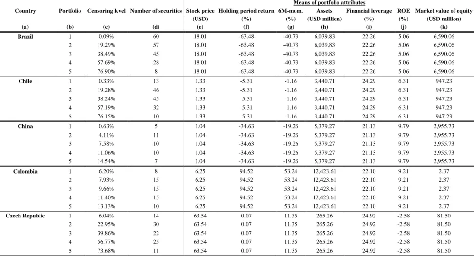
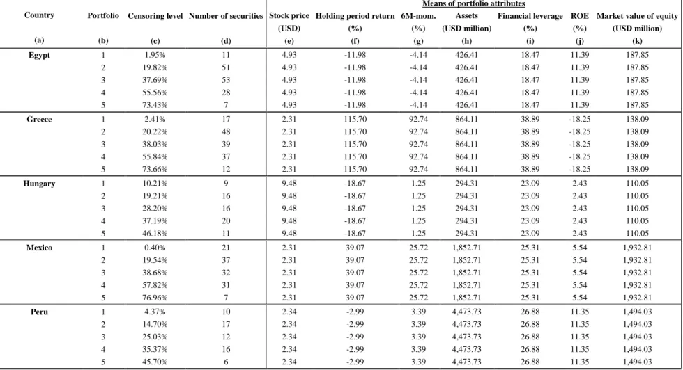
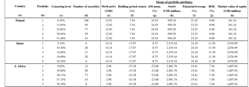
(7) vi. INDICE DE TABLAS. Table 1. Descriptive statistics by country ...................................................................... 233 Table 2a. Mean beta estimates by country using an equally weighted index .................. 26 Table 2b. Mean beta estimates by country using a value weighted index ....................... 27 Table 3. Median country spread between maximum and minimum beta estimates and percentage improvement over OLS beta .................................................................. 31 Table 4a. Beta rankings based on max-min portfolio spread, equally weighted index ... 34 Table 4b. Beta ranking based on max-min portfolio spread, value weighted index ........ 35 Table A.1 Number of firms per country........................................................................... 41 Table A.2.a Portfolio formation: summary of portfolio attributes ................................... 42 Table A.2.b Portfolio formation: summary of dispersion of portfolio attributes ............. 45 Table A.3.a Portfolio betas by country using an equally weighted index........................ 48 Table A.3.b Portfolio betas by country using a value weighted index ............................ 50. vi.

(8) vii. RESUMEN. Un aspecto importante de la valorización de activos es la correcta determinación de una medida de riesgo. El modelo de mercado es la herramienta usual ocupada para ello. De acuerdo a este modelo, existe una relación lineal entre el retorno de un activo y el retorno del mercado. El coeficiente que se genera a partir de esta relación se denomina beta, y mide la exposición a riesgo sistemático del activo. Para llegar a este coeficiente, una regresión de mínimos cuadrados (OLS) es generalmente realizada. Cuando un activo se transa con menor frecuencia en comparación al mercado, la medida de riesgo que entrega la regresión OLS tiende a estar sesgada a la baja, pues presenta “thin trading bias”. Este resultado es especialmente relevante en mercados emergentes, en donde el volumen de acciones transado suele ser menor que en otros mercados más desarrollados. Varios ajustes han sido propuestas en la literatura para corregir este sesgo, pero aún no existe un consenso generalizado sobre cuál de todos es el más efectivo. Esta tesis compara el comportamiento de los ajustes existentes aplicados a un grupo significativo de mercados emergentes, con el objetivo de determinar cuál de todos es el más efectivo en la corrección del sesgo. Para. ello, y a partir de un modelo de. programación lineal, se generan portafolios con igual niveles de riesgo, pero cuyos activos no se transan con la misma frecuencia. Dado que el parámetro beta es una medida de riesgo sistemático, si es que mantenemos constante el nivel de riesgo a lo largo de los portafolios, entonces los betas resultantes deberían ser aproximadamente iguales. Esto nos permite generar una manera de comparar los distintos ajustes, ya que el mejor es aquel que entrega los betas más similares entre portafolios. Los resultados muestran que los betas que se estiman ocupando retornos basados en transacciones que efectivamente ocurrieron son los más efectivos. Específicamente, el ajuste del tipo “sample selectivity” es, en general, el que muestra un mejor desempeño y entrega hasta un 41% de mejora por sobre betas calculados ocupando OLS.. Palabras claves: mercados emergentes, thin trading, estimación de riesgo, beta vii.

(9) viii. ABSTRACT. Risk calculation, in the form of beta estimation, is a key aspect of asset valuation. When assets do not trade as frequently as the market portfolio, the standard OLS beta exhibits thin trading bias. Several beta adjustment techniques exist to correct for this bias; however, no consensus exists as to which adjustment is best. This paper compares the behavior of the most widely used beta adjustments proposed in the literature in a comprehensive group of emerging markets. Using a linear programing model, we form portfolios with equal risk characteristics, but different levels of censoring. Since beta is a measure of systematic risk, if most risk factors are kept constant across portfolios, the resulting betas should be approximately the same. Our results show that beta adjustments based on trade-to-trade returns perform best. Specifically, the best overall adjustment is the sample selectivity adjustment, which provides up to a 41% improvement over OLS betas.. Keywords: emerging markets; thin trading; risk estimation; beta JEL classification: C1; C6; C52; G0; G1; G1. viii.

(10) 1. 1.. Introduction. An important aspect of asset valuation is the determination of discount rates, which requires an appropriate measure of risk. The market model is the fundamental method for estimating such a risk measure (Scholes & Williams, 1977). According to this model, a linear relationship exists between an asset’s return and the return on the market portfolio; the coefficient of this linear relationship is known as beta and measures the asset’s exposure to systematic risk. By running an OLS regression on the past returns of the asset against those of the market, we obtain an estimation of the beta coefficient. Various other risk estimation methodologies build upon the market model’s notion that an asset’s return is related to – and can be explained through its sensitivity to – one or more risk factors.1 The market model yields reasonable results for assets traded in developed countries with liquid markets (Brooks, Faff, Fry, & Bissoondoyal-Bheenick, 2005). However, as we delve into markets with low trading volumes, where an asset may spend days, weeks, or even months without being traded, the OLS beta begins to falter, exhibiting a downside bias (Bartholdy & Riding, 1994; Beer, 1997; Berglund, Liljeblom, & Löflund, 1989; Dimson, 1979; Scholes & Williams, 1977; Sercu, Vandebroek, & Vinaimont, 2008). This illiquidity problem is common in emerging markets (Antoniou, Ergul, & Holmes, 1997; Beer, 1997; Iqbal & Brooks, 2007); given that many investors’ attention is fixated on these markets (Buchanan, English, & Gordon, 2011; De-la-Hoz & Pombo, 2016; Pereiro, 2001), it is especially relevant to find a way to correctly estimate and quantify their firms’ risk. The relevance behind correctly estimating risk rests upon its common use in valuation. If an incorrect, or biased, measure of beta is used as input when estimating discount rates,. 1. See, among others, the Capital Asset Pricing Model (Lintner, 1965; Sharpe, 1964), or multi-factor models,. such as Fama and French’s three-factor model (Fama & French, 1993) or the four-factor model proposed by Hou, Xue, and Zhang (2015)..

(11) 2. the resulting rate will be distorted. In the context of emerging markets, as betas that present thin trading bias are usually downward biased, the discount rate that is obtained will also be lower. This will yield a valuation that is upwards biased, as the present value of an asset is inversely proportional to the discount rate used, resulting in assets that are overvalued. This result has important implications in areas related to finance and project valuation, where a biased beta estimate can result in the incorrect approval of projects. Various authors have developed beta adjustments that deal with thin trading bias; however, no consensus exists as to which is the most effective. Moreover, many studies present contradictory results.2 We contend that the lack of general consensus is, at least partially, due to the fact that the comparison methodologies used to date in the literature are not fully adequate. Furthermore, most antecedents try to establish which adjustment works better in a given market, but do not address the question of beta behavior in a comprehensive group of markets. In this paper, we analyze and compare the various beta adjustment techniques derived in the literature by applying them to stocks belonging to a significant, complete, and independently defined group of emerging markets. We base our comparison on the use of a linear programming model that forms portfolios with equal risk factors, but different. 2. Berglund et al. (1989) study various correction procedures using daily data from the Finnish equity market,. and conclude that none of the adjustments generate a material improvement over the traditional market model. Bartholdy & Riding (1994) study the New Zealand equity market, and establish that OLS betas are less biased than, more efficient than, and as consistent as the Dimson and Scholes-Williams estimators. Meanwhile, Fowler, Rorke, and Jog (1989) conclude, using a theoretical approach, that Dimson and Scholes-Williams estimates are less biased, but also less efficient, than OLS estimates. Luoma et al. (1994) conclude that trade-to-trade betas appear to yield satisfactory results when applied to the Stockholm Stock Exchange, while Beer (1997) concentrates on the Belgian equity market and states that simple OLS beta estimates seem to work well in comparison with other adjustments. Finally, Brooks et al. (2005) find that both Dimson and sample selectivity betas are able to effectively correct the downward bias arising in the OLS beta from thin trading in the Canadian market..

(12) 3. levels of censoring.3 Specifically, the model takes into consideration known risk factors that can affect an asset’s return, such as size, value, momentum, and quality (Asness, 1995; Asness, Frazzini, & Pedersen, 2017; Banz, 1981; Basu, 1977; Fama & French, 1993; Rosenberg, Reid, & Lanstein, 1985), and equalizes them across portfolios while maintaining different levels of censoring. Given that beta is a measure of systematic risk, if most risk factors are held constant across a set of portfolios, their beta estimates should be approximately the same. In other words, any differences in the portfolios’ betas should emanate solely from the differences in their censoring. Therefore, the best adjustment is that which yields the most similar betas across portfolios. We estimate betas based on daily returns for MSCI’s list of emerging countries for which we have complete data.4 Specifically, we compare the following beta adjustments: (i) the Scholes and Williams estimator (Scholes & Williams, 1977); (ii) the trade-to-trade beta adjustment (Marsh, 1979); (iii) the adjusted coefficients method (Dimson, 1979); (iv) the correction to Dimson’s adjustment proposed by Fowler and Rorke (Fowler & Rorke, 1983); (v) the Cohen-Hawanini-Maier-Schwartz-Whitcomb (CHMSW) method (Cohen, Hawawini, Maier, Schwartz, & Whitcomb, 1983); and (vi) the sample selectivity model put forward by Brooks et al. (2005). For every country, we form five portfolios with equal risk characteristics but different levels of censoring. Our initial results confirm the presence of thin trading bias in OLS estimates across all of the emerging markets we focus on. Specifically, we observe a steady decline in the OLS beta estimate as we move from portfolios with higher levels of censoring to those with lower levels of censoring within each country. Such bias diminishes when we employ the adjustment procedures.. 3. We measure the level of censoring as the ratio between the number of days during which a stock is not. traded and the total number of trading days during a given time period. 4. MSCI stands for Morgan Stanley Capital International..

(13) 4. To rank the effectiveness of different adjustments within each country, we consider the spread between the maximum and minimum portfolio betas that each adjustment yields.5 The lowest spread indicates the best adjustment, since it delivers the most similar betas across portfolios. When the beta adjustments are compared among each other, we find that betas that compute returns on a trade-to-trade basis – namely, the sample selectivity, Scholes-Williams, and trade-to-trade betas – show the best results using both equally weighted and value weighted market portfolios.6 When we use an equally weighted index as the market portfolio, we find that all adjustments outperform the OLS method. The sample selectivity and trade-to-trade adjustments perform best, presenting 41% and 35% average improvements over OLS, respectively. In contrast, when we use a value weighted index as the market portfolio, the adjustments do not always outperform the OLS method. Consistent with previous studies, betas estimated through a value weighted index generally tend to be lower than those based on an equally weighted index. Moreover, the use of a value weighted index seems to diminish some of the thin trading bias present in emerging markets. Therefore, a valid alternative to the use of trade-to-trade methods to correct for this bias could be simply using the OLS method on a value weighted index. This manuscript is structured as follows: Section 2 explains the most commonly used adjustments proposed in the literature to control for thin trading bias; Section 3 outlines the methodology used to compare these beta adjustments; Section 4 describes the data; Section 5 provides the results; and Section 6 concludes.. 5. For every country, we form five portfolios and estimate their betas according to each adjustment. Thus,. every country has 5 estimates of beta per adjustment. 6. The Scholes-Williams and sample selectivity adjustments use daily returns only when stocks were traded. on two consecutive days. Meanwhile, the trade-to-trade adjustment uses returns that are computed on any adjacent trades, regardless of the time between them, and scales them by a factor reflecting the length of the interval on which these returns were computed. The three adjustments, therefore, compute returns only for days in which transactions have occurred; for this reason, we refer to them as trade-to-trade methods..

(14) 5. 2.. Related literature. Various adjustments for minimizing thin trading bias have been proposed in the literature; however, it is yet not clear which performs best. In this section, we first describe the OLS regression that is typically used to estimate betas in the market model (Section 2.1). Then, in 2.2, we review the most commonly used adjustment procedures: (i) the Scholes and Williams estimator; (ii) the trade-to-trade beta adjustment; (iii) the adjusted coefficients method; (iv) the Fowler-Rorke method; (v) the Cohen-Hawanini-Maier-SchwartzWhitcomb (CHMSW) method (Cohen et al., 1983); and (vi) the sample selectivity model.7 Finally, in 2.3, we provide an overview of how the aforementioned methods have been previously compared in the literature.. 2.1 OLS beta The standard OLS beta is the fundamental method for estimating an asset’s systematic risk. According to the market model, there is a linear relationship between the expected value of the returns of an asset, 𝑅𝑗,𝑡 , and those of the market portfolio, 𝑀𝑡 . By running an OLS regression of the asset’s returns on the returns of the market (see Eq. 1), we are able to estimate the asset’s beta (𝛽𝑗 ).8 This approach calculates returns between all pairs of consecutive trading days over a sample period, irrespective of whether the asset was traded on those days or not. 𝑅𝑗,𝑡 = 𝛼 + 𝛽𝑗𝑂𝐿𝑆 𝑀𝑡 + 𝜀𝑗,𝑡 7. (1). Additional corrective procedures have been proposed in the literature. However, they usually require prior. knowledge of an asset’s underlying return distribution, and therefore, are not widely used. See, for example, Fowler, Rorke, & Jog (1989) and Vasicek (1973). 8. The market model uses a regression that is very similar to the one used in the Capital Asset Pricing Model.. However, the market model uses absolute returns, rather than excess returns, for both the asset and the market..

(15) 6. As mentioned in Section 1, however, the standard OLS method can lead to biased beta estimates when applied to assets that are traded infrequently ( Dimson, 1979; Scholes & Williams, 1977). In particular, assets that trade less frequently than the market, on average, exhibit consistently lower beta estimates than frequently traded stocks (Cohen et al., 1983; Dimson, 1979; Scholes & Williams, 1977). Due to the existence of this bias, the OLS beta estimation technique is sometimes used as an upper bound to which potential adjustments are compared.9. 2.2 Thin trading adjustments. In the following subsections, we enumerate and describe the most common beta adjustments proposed in the literature. 2.2.1. Scholes-Williams estimator. The Scholes-Williams beta (Scholes & Williams, 1977) is calculated by running three separate regressions of an asset’s returns on lagged, leading, and synchronous market returns, respectively, as in Eq. 2. The Scholes-Williams estimator is given by the sum of the beta coefficients resulting from these three regressions, divided by one plus two times the first-order autocorrelation, 𝜌1 , of the market return (see Eq. 3). 𝑅𝑗,𝑡 = 𝛼 + 𝛽𝑗 𝑀𝑡+𝑘 + 𝜀𝑗,𝑡 , 1. 𝛽𝑗𝑆𝑊 = ∑ 𝑘=−1. 9. 𝑘 = −1,0,1. 𝛽𝑘 1 + 2𝜌1. (2) (3). Such a methodology has been used by McInish & Wood (1986), Berglund et al. (1989), Bartholdy &. Riding (1994), and Beer (1997), among others, with no consensus as to which adjustment best accounts for thin trading bias..

(16) 7. Unlike the OLS method, this approach calculates and uses a return only if transactions have occurred on two consecutive trading days. This restriction usually results in a loss of observations available for use, thus making it inefficient compared to other beta adjustments (Dimson, 1979).10. 2.2.2. Trade-to-trade beta adjustment. The trade-to-trade beta, proposed by Marsh (1979), is similar to the Scholes-Williams beta in that it calculates and uses a return only if transactions occur. However, it abandons the requirement for consecutive trading days and instead uses returns computed on adjacent trades over a period of any length. To avoid the rise of any heteroscedasticity problems, it scales each return by a factor of 1⁄√𝑑𝑡 , in which 𝑑𝑡 corresponds to the number of trading days between the consecutive trades used to compute that return. Consistently, it computes the market returns over the same periods of time as the asset returns, and then regresses the adjusted asset returns on the synchronous adjusted market return, as follows: 𝑅𝑗,𝑡 √𝑑𝑡. = 𝛼 + 𝛽𝑗𝑇𝑇 (. 𝑀𝑡 √𝑑𝑡. ) + 𝜀𝑗,𝑡. (4). 2.2.3. Dimson’s adjusted coefficients method Dimson’s adjusted coefficients method, hereafter referred to as the Dimson adjustment, involves running a regression model of an asset’s returns on leading, synchronous, and lagged market returns simultaneously, as in Eq. 5. The Dimson beta is calculated by summing up all of the estimated beta coefficients obtained from the aforementioned regression, as shown by Eq. 6.. 10. Efficiency refers to the relation between variance and number of observations. In this sense, the most. efficient estimator would be that which has the smallest variance given a fixed sample size..

(17) 8. 𝑛. 𝑅𝑗,𝑡 = 𝛼 + ∑ 𝛽𝑘 𝑀𝑡+𝑘 + 𝜀𝑗,𝑡. (5). 𝑘=−𝑛 𝑛. 𝛽𝑗𝐷𝐼𝑀. = ∑ 𝛽𝑘. (6). 𝑘=−𝑛. The more thinly traded an asset, the more the parameter 𝑛 must increase in order to reduce the thin trading bias (Dimson, 1979). To what extent this parameter must be increased is, however, left to the user to determine. In his study, Dimson chooses to use five leads and lags, though he conducts no further studies to determine the optimal number of nonsynchronous coefficients to use. In choosing this number, we incur a trade-off between accuracy and statistical efficiency. In effect, as the parameter 𝑛 increases, the model becomes more accurate and realistic, but the efficiency of the estimator declines (Cohen, Hawawini, Maier, Schwartz, & Whitcomb, 1983).. 2.2.4. Fowler-Rorke beta Fowler & Rorke (1983) demonstrate that Dimson’s estimator is not consistent with that of Scholes and Williams and provide a corrected version of the former. The method relies on the same regression established in Eq. 5; however, the resulting beta is computed as a weighted sum of the estimated beta coefficients, as in Eq. 7.. 𝑛. 𝛽𝑗𝐹𝑅. = ∑ 𝑤𝑘 𝛽𝑘 , 𝑛 ∈ {1,2}. (7). 𝑘=−𝑛. 𝑤1 = 𝑤−1 = 𝑤2 = 𝑤−2 =. 1 + 𝜌1 1 + 2𝜌1. 1 + 𝜌1 + 𝜌2 1 + 2𝜌1 + 2𝜌2. (8).

(18) 9. Eq. 5, 7, and 8 consider up to two leading and lagging terms, in line with what Fowler & Rorke proposed and used in their study.. 2.2.5. CHMSW method. Cohen et al. (1983) develop a correction procedure that also uses multiple leads and lags. Eq. 9 and 10 formally describe how to apply their method. By including multiple leads and lags, they show theoretically that the bias in beta decreases as the length of the measurement interval increases, monotonically approaching zero. 𝛽𝑗𝐶𝐻𝑀𝑆𝑊. 𝛽0 + ∑𝑛𝑘=1 𝛽+𝑘 + ∑𝑛𝑘=1 𝛽−𝑘 = 1 + ∑𝑛𝑘=1 𝜌+𝑘 + ∑𝑛𝑘=1 𝜌−𝑘. (9). 𝑐𝑜𝑣(𝑅𝑗,𝑡 , 𝑀𝑡 ) 𝑣𝑎𝑟(𝑀𝑡 ). (10a). 𝛽+𝑘 =. 𝑐𝑜𝑣(𝑅𝑗,𝑡+𝑘 , 𝑀𝑡 ) 𝑣𝑎𝑟(𝑀𝑡 ). (10b). 𝛽−𝑘 =. 𝑐𝑜𝑣(𝑅𝑗,𝑡−𝑘 , 𝑀𝑡 ) 𝑣𝑎𝑟(𝑀𝑡 ). (10c). 𝜌+𝑘 =. 𝑐𝑜𝑣(𝑀𝑡+𝑘 , 𝑀𝑡 ) 𝑣𝑎𝑟(𝑀𝑡 ). (10d). 𝜌−𝑘 =. 𝑐𝑜𝑣(𝑀𝑡−𝑘 , 𝑀𝑡 ) 𝑣𝑎𝑟(𝑀𝑡 ). (10e). 𝛽0 =. 2.2.6. Sample Selectivity Model. Brooks et al. (2005) argue that, in cases of extreme illiquidity, a superior means of estimating betas is one that separates the treatment of zero and non-zero daily returns in the sample. Therefore, the method includes two stages. The first stage consists of a probit.

(19) 10. model that deals with the appearance of zero returns in the observed data. In this stage, the method assumes that, underlying the observed data, there exists a latent variable that can be explained via a certain covariate, such as trading volume. If, on a given day, this covariate exceeds some threshold, the method assumes there is a valid non-zero return. The second stage applies to the valid non-zero returns identified in the first stage. In this second stage, an OLS regression similar to Eq. 1 is run on these non-zero returns. The main difference with respect to the standard OLS regression is that the sample selectivity model incorporates a second covariate, known as the Inverse Mill’s Ratio, to accompany the market return in Eq. 1. This is done to correct for the selectivity bias that might have been introduced during the first stage.11. 2.3 Comparison between adjustments. So far, we reviewed the most relevant adjustment techniques proposed in the literature. In this subsection, we revise the main methodologies used to compare the results that these adjusting procedures produce. As the true beta of an asset is unobservable, we cannot rank adjustments based on how close they are to the true beta. We identified four primary beta comparison techniques in the literature: (i) a statistical approach; (ii) the examination of beta stability; (iii) the use of data simulation; and (iv) direct comparison with OLS betas. 2.3.1. Statistical approach. Many studies have addressed the question of beta behavior from a statistical point of view, focusing on areas such as the efficiency and the statistical significance of the estimators. Dimson (1979) is one of the first to address the question of how efficient a beta estimator is. He simulates a database of 100 securities with different trading frequencies that depend on the firms’ market capitalizations.. 11. For further discussion of the sample selectivity model, see Brooks et al. (2005)..

(20) 11. Dimson then estimates betas using the OLS method, as well as via the Scholes-Williams, trade-to-trade, and Dimson adjustments. He computes average betas for each decile of trading frequency and finds that, even though the trade-to-trade adjustment slightly overestimates beta, it is relatively efficient, whereas the Scholes-Williams estimator is very inefficient. Davidson & Josev (2005) measure the statistical significance of the Scholes-Williams, Dimson, and Fowler-Rorke adjustments. They focus on Australian stocks and estimate the adjustments using a five-year period of daily returns. To determine the statistical significance of these adjustments, Davidson & Josev determine the number of beta estimates that are statistically different from the OLS betas. They conclude that many of the adjustments do not add any statistical value, as they are not statistically different from OLS betas. A takeaway from these studies is that a statistical approach does not yield definitive conclusions regarding which beta estimation adjustment is best. From a statistical point of view, efficiency of the estimator is a desirable property. However, by focusing only on efficiency or statistical significance we fail to address the question of whether the adjustments properly correct for thin trading bias or not. That a certain estimator is more efficient than, or statistically different from, another does not necessarily mean that it is less biased. 2.3.2. Examination of beta stability If no major changes in a company or industry occur, one would expect a firm’s beta to be relatively consistent over time. In this sense, a reliable estimator would be one that shows the most stability during a given sample period. Several studies have focused on the stability of risk measures in thin markets.12. 12. See, among others, Clare, Morgan, & Thomas (2002), Dimson & Marsh (1983), and Marsh (1979)..

(21) 12. However, examining the stability of betas could be a misleading way of comparing them, especially in the presence of thin trading. Provided that trading frequency is serially correlated, and that thinly traded shares have low beta estimates while frequently traded shares have high estimates, thin trading causes betas to appear more stable over time than they really are (Berglund et al., 1989; E. Dimson & Marsh, 1983; Dimson, 1979). This makes it difficult to compare the quality of alternative beta adjustments solely by examining their stability or comparing this stability with that of OLS betas. Moreover, an increase in beta stability does not necessarily mean that the adjustment procedure is successful in eradicating thin trading bias. 2.3.3. Use of simulated data. Another methodology proposed for comparing adjustments is the use of simulated data to artificially create thinly traded assets. For instance, as discussed in a previous section, Dimson (1979) uses a simulated database to compare various adjustments. An alternative approach is used by Luoma et al. (1994). By randomly removing daily observations of stocks belonging to the Stockholm Stock Exchange, Luoma et al. artificially create markets with levels of censoring ranging between 10 and 30 percent. They report that different beta adjustments behave differently according to the level of censoring, and conclude that the effectiveness of the beta adjustments varies across markets depending on this level. When using simulated data, either in the form of a simulated database or one based on manipulated data, it is impossible to ensure that results will hold with the use of real data (McInish & Wood, 1986). Moreover, real data might include the appearance of zero returns in a non-random fashion, and therefore, the random removal of observations might yield impractical datasets. 2.3.4. Comparison of the adjustments with the OLS estimate.

(22) 13. A fourth approach considers comparing the adjustments directly with the OLS estimate. Dimson (1979) is one of the first to study the effectiveness of this technique on simulated and real data, the latter collected from the London Stock Exchange. Since larger companies trade, on average, more frequently than smaller ones, Dimson assigns the stocks to deciles according to their market value and computes an average beta for each group. He observes a much more even distribution of estimated betas across deciles of market value when the Dimson adjustment, rather than the OLS method, is used. Thus, he concludes that this adjustment seems to eliminate most of the thin trading bias present in beta estimation. However, despite showing that his adjustment at least partially addresses the bias, Dimson’s analysis does not compare it with other potential adjustments. Brooks et al. (2005) compare the OLS approach with the Dimson and sample selectivity adjustments. They rank stocks to group them according to three categories: (i) level of censoring; (ii) firm size, as proxied by market value of equity; and (iii) trading volume. They confirm the existence of a negative relationship between censoring and firm size, and between censoring and trading volume. In effect, as the degree of censoring increases, firm size and trading volume fall. In addition, they find that, across the three categories mentioned, both Dimson and sample selectivity betas tend to be higher than the OLS beta, effectively correcting its downward bias. This conclusion, however, fails to address the question of which adjustment better accounts for such bias. The adjustment that increases the beta estimate the most is not necessarily correct, as it may overestimate the stock’s risk. The same type of ranking approach is applied by Brooks et al. (2014) to select Latin American countries13, and by Iqbal & Brooks (2007) to the Pakistani market. In summary, it is safe to conclude that prior studies have not come to a general consensus as to which beta adjustment works best. While some authors posit that the trade-to-trade (Luoma et al., 1994) or Dimson (McInish & Wood, 1986) adjustments are able to effectively account for thin trading bias, others establish that no adjustment provides substantial incremental benefits to the standard OLS method (Bartholdy & Riding, 1994; 13. Argentina, Brazil, Chile, Mexico, Colombia, Peru, and Venezuela..

(23) 14. Berglund et al., 1989; Davidson & Josev, 2005). We contend that these inconsistencies are partially due to the lack of an adequate framework of comparison, and to the fact that most studies focus on a single market or a small number of markets, thus encountering problems of generalizability. In this paper, we use a methodology that overcomes these shortcomings and provides a better setting for testing the various beta adjustments. This methodology is adapted from McInish & Wood (1986) and rests upon the notion that beta is a measure of systematic risk and, therefore, portfolios with very similar risk characteristics should exhibit very similar betas. Specifically, by creating portfolios with equal risk characteristics – such as size, value, momentum, and quality – but different levels of censoring, we are able to ascertain which beta adjustment is most effective by determining which yields the most similar results across portfolios.. 3.. Methodology. In this section, we review the methodology and rationale behind our portfolio formation process. Following McInish & Wood (1986), we estimate betas over a portfolio holding period of two years, which is centered in a four-year sample period used to compute risk factors. The portfolio holding period overlaps with the sample period, but the sample period includes an extra year before and after in order to provide more data on the risk factors, some of which are computed annually.. 3.1 Linear programming model. We use a linear programming model to create portfolios with equal risk characteristics but different levels of censoring in order to analyze and compare the various beta adjustments. As we previously stated, the degree of censoring proxies for a stock’s illiquidity and is computed during the portfolio holding period as the ratio between the number of days a stock is not traded and the total number of trading days. Section 3.1.1 enumerates the.

(24) 15. factors incorporated into the linear programming model, while Section 3.1.2 formulates and explains the model. 3.1.1. Risk factors There is a vast literature documenting the risk factors that can affect a stock’s return. We consider size, value, momentum, and quality, as they are the most commonly accepted and used factors. Size A company’s size explains a stock’s expected return, even after adjusting for other sources of systematic risk (Banz, 1981; Fama & French, 1993). Because smaller companies are more vulnerable than larger, established firms with solid track records, smaller firms tend to have higher returns than their larger counterparts (Banz, 1981; Fama & French, 2012; Pereiro, 2001). We incorporate this factor by holding the market value of equity and book value of assets approximately equal among portfolios. Each portfolio's market value of equity and book value of assets is computed as the average of these values for its constituent stocks. Value The value factor captures the relationship between a stock’s price and its fundamental value (Basu, 1977; De Bondt & Thaler, 1986; Rosenberg et al., 1985). As discussed in the previous paragraph, we hold the average market value of equity and book value of assets approximately equal across portfolios. With this, we also ensure that the portfolios have similar price-to-book ratios, which is a known value metric (Asness, Moskowitz, & Pedersen, 2013). Momentum Momentum measures excess returns to stocks with stronger past performance (Asness, 1995; De Bondt & Thaler, 1985; Jegadeesh & Titman, 1993). In effect, Jegadeesh & Titman (1993) show that trading strategies that select stocks on the basis of their performance during the past months yield positive future returns. We include momentum.

(25) 16. by considering the average return of each portfolio during the six months prior to the holding period (Asness, Moskowitz, & Pedersen, 2013). Quality The quality factor aims to capture the excess return associated with companies of better quality (Asness et al., 2017). We proxy for this factor through each company’s level of financial leverage, measured as the ratio of total debt to total assets, and its return on equity (ROE). The financial leverage and ROE of each portfolio are then calculated as the averages of these values among its constituent stocks. Additional portfolio characteristics In addition to controlling for the aforementioned systematic factors, and following McInish & Wood (1986), we also keep each portfolio’s overall return and the average prices of its stocks approximately equal. The portfolio’s overall return is computed as the mean holding period return of its constituent stocks throughout the holding period, and it is included since riskier diversified portfolios should generate larger returns, on average.. 3.1.2. Model formulation. The linear programming model seeks to create five homogenous portfolios across risk dimensions that differ in their levels of censoring. To achieve this, the model’s objective function maximizes the difference in censoring between extreme portfolios, while holding the difference in censoring between adjacent portfolios approximately equal. Moreover, the model forms portfolios not only with equal risk characteristics on average, but also with similar dispersion. In other words, we constrain the model to create portfolios that are equal at the mean and dispersion levels of the risk factors described in Section 3.1.1. Formally, the linear programming model is formulated as follows:.

(26) 17. 𝑉 max (∑ 𝑤1,𝑗 𝑐𝑗 − ∑ 𝑤5,𝑗 𝑐𝑗 ) −𝑀𝑀 ∑ Δ𝑀 𝑛 − 𝑀𝑉 ∑ Δn. 𝑖,𝑗,𝑛 ∈ 𝑁. 𝑗. 𝑗. 𝑛. (1). 𝑛. ∑ 𝑤𝑖−𝑘,𝑗 𝑐𝑗 − ∑ 𝑤𝑖−𝑘−1,𝑗 𝑐𝑗 𝑗. s.t.. 𝑖 = 1, … ,5. 𝑗. = ∑ 𝑤𝑖−𝑘−1,𝑗 𝑐𝑗 − ∑ 𝑤𝑖−𝑘−2,𝑗 𝑐𝑗 𝑗. 𝑘 = 1, 2, 3. (2). 𝑗. ∑ 𝑤𝑖,𝑗 𝑎𝑛,𝑗 = ∑ 𝑤𝑘,𝑗 𝑎𝑛,𝑗 ± ΔM 𝑛 𝑗. 𝑗. ∀𝑛 ∀𝑖 ≠𝑘. (3). ∑ ∑(𝑤𝑖,𝑗 𝑎𝑛,𝑗 − 𝑤𝑖,𝑙 𝑎𝑛,𝑙 ) 𝑗. ∀𝑛. 𝑙>𝑗. = ∑ ∑(𝑤𝑘,𝑗 𝑎𝑛,𝑗 − 𝑤𝑘,𝑙 𝑎𝑛,𝑙 ) ± ΔV𝑛 𝑗. 𝑙>𝑗. ∑ 𝑤𝑖,𝑗 ≥ 0.01. ∀𝑖 ≠𝑘. (4). 𝑙∈𝑁. ∀𝑗. (5). 𝑤𝑖,𝑗 ≤ 0.3. ∀ 𝑖, 𝑗. (6). ∑ 𝑤𝑖,𝑗 = 1. ∀𝑖. (7). 𝑖. 𝑗.

(27) 18. In this model, 𝑤𝑖,𝑗 represents the weight of stock 𝑗 in portfolio 𝑖 ∈ {1,5}, 𝑐𝑗 is the level of censoring of stock 𝑗, and 𝑎𝑛,𝑗 refers to the 𝑛-th attribute associated with the risk factors of stock 𝑗.14 As we have already established, the objective function maximizes the difference in censoring between extreme portfolios. Through the objective function, we also determine appropriate delta values to be used as tolerance margins in the model’s constraints: ΔM 𝑛 for the constraints relating to the mean level of the risk attributes and ΔV𝑛 for those relating to the dispersion of such characteristics. These deltas ensure that the model attains feasibility while maintaining the mean and dispersion of the risk characteristics as similar as possible between each portfolio. As to the model restrictions, constraint (2) holds the difference in censoring between adjacent portfolios equal. Constraint (3) keeps the mean levels of the risk attributes approximately equal between the various portfolios, while constraint (4) maintains the dispersion of these risk attributes approximately equal across portfolios.15 Constraint (5) ensures that all of the stocks in the sample are used at least once in a portfolio. Through this inequality, we also comply with non-negativity of weights.16 14. As mentioned earlier, these attributes are the following: (i) market value of equity; (ii) book value of. assets; (iii) average stock price; (iv) 6-month momentum; (v) financial leverage; (vi) ROE; and (vii) mean holding period return. 15. Through constraints (3) and (4), we force the model to create portfolios that are similar across the defined. risk dimensions, thus ensuring that the portfolios are balanced. In the absence of constraint (4), the linear programming model could yield portfolios that are, on average, similar, but have significantly different dispersion across the various dimensions. For example, the model could combine very high- and low-priced stocks, and very small and large firms, if this yields an increase in the objective function. On average, these portfolios would be similar, but in fact they would be formed by very dissimilar assets, which could tamper with the model’s purpose of yielding portfolios with similar risk characteristics. 16. Non-negativity of weights implies that only long positions can be held in the stocks. This is done for. simplicity and does not result in loss of generality, since we are concerned with forming portfolios with equal risk characteristics rather than optimal asset allocation..

(28) 19. Constraint (6) restricts the maximum weight of any stock to 30%, thus ensuring that no stock holds a higher proportion in any portfolio.17 Finally, constraint (7) ensures that the sum of the weights in each portfolio is one. Given the model’s solution, we calculate each portfolio’s beta as the weighted sum of the betas of its constituent stocks. As we mentioned earlier, we argue that the beta adjustment technique that performs best is the one that gives most homogeneous results across the portfolios.. 4.. Data. We investigate the extent of thin trading bias and the relative merit of each adjustment using stocks from several emerging markets. We seek to establish which adjustment is best suited for estimating betas within each country; we also explore whether an overall pattern exists, in the sense that one or more beta adjustments systematically perform better in all emerging markets. As emerging markets are usually characterized by illiquidity, they provide an ideal setting for comparing the adjustments.. 4.1.. Emerging markets and sample period. We use MSCI’s definition to identify emerging markets. Every year, MSCI revises each country’s status based on its economic development, economy size, liquidity, and the. 17. A lower limit would help create more diversified portfolios. However, some countries in our sample only. have a few stocks with complete data; therefore, the use of a lower limit tended to generate feasibility problems in the model..

(29) 20. accessibility of its markets. With this information, it categorizes the countries into frontier, emerging, and developed countries to form MSCI Markets Indexes.18 We use 2012-2015 as the sample period to compute risk factors and 2013-2014 as the portfolio holding period to estimate beta adjustments. Therefore, our initial sample comprises publicly traded firms belonging to the 22 emerging markets that were part of the MSCI Emerging Markets Index at some point during the portfolio holding period: Brazil, Chile, China, Colombia, the Czech Republic, Egypt, Greece, Hungary, India, Indonesia, Malaysia, Mexico, Peru, Philippines, Poland, Qatar, Russia, South Africa, South Korea, Taiwan, Thailand, and Turkey. To the best of our knowledge, no previous studies include such an extensive list of countries.. 4.2.. Main variables. To account for the risk factors previously described in Section 3.1.1, we rely on daily stock market information and annual accounting information from Bloomberg. The raw data sample includes all firms for which the daily adjusted price of common stock was available during the whole portfolio holding period.19 We compute returns as the logarithmic difference in adjusted prices (Cohen et al., 1983; Dimson, 1979). The number of trading days used to compute returns depends on the type of adjustment used, as described in Section 2.2. For the Dimson, Fowler-Rorke, and CHMSW adjustments, we use consecutive trading days, even if prices did not change due 18. For a country to be considered emerging, it must have significant openness to foreign ownership and ease. of capital inflows and outflows, the efficiency of its operational framework must be adequate, and its institutional framework must be at least modestly stable. Regarding firm size and liquidity, the country must have at least three companies with a market capitalization of USD 898 million or larger, another three companies with a market capitalization of USD 449 million or larger, and 15% or higher ATVR (Annualized Traded Value Ratio, a measure of the percentage of total share value that trades every day). 19. Daily price is adjusted to reflect spin-offs, stock splits or consolidations, stock dividends, and rights. offerings..

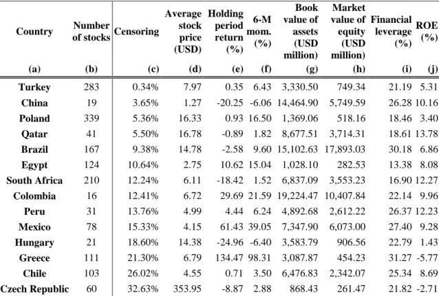
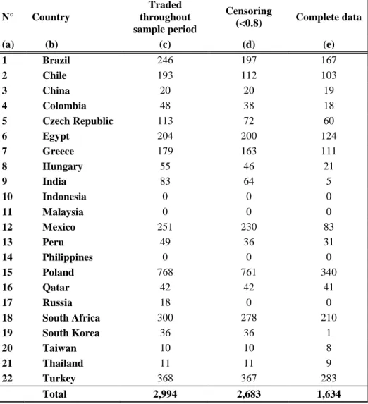
(30) 21. to thin trading. In contrast, the Scholes-Williams and sample selectivity adjustments use daily returns only when stocks were traded on two consecutive days. Finally, the trade-totrade adjustment uses stock returns that are not necessarily computed on consecutive days. In effect, the trade-to-trade adjustment considers stock returns computed on adjacent trades of any length, and scales them by a factor to reflect the length of the interval on which these returns are computed. Even though the computations differ between the Scholes-Williams, sample selectivity, and trade-to-trade adjustments, all of these methods only consider returns when a transaction, or trade, occurs; therefore, we assert that their returns are computed on a trade-to-trade basis. For all stocks, we obtained daily trading volume for the aforementioned time period. The daily trading volume allows us to measure each stock’s level of censoring. Following Brooks et al. (2005; 2014), and to prevent extreme beta estimates, we filtered the list of stocks to rule out any companies with a censoring level of 80% or above.20 We measure the market value of equity on the last trading day prior to the beginning of the portfolio holding period. We calculate the book value of assets, financial leverage, and ROE as the means of their annual values over the sample period. We calculate the average daily stock price and holding period return of each stock over the portfolio holding period. Finally, we compute the momentum of each stock by considering its return during the six months prior to the beginning of the portfolio holding period.. 4.3.. Final sample. Our final sample includes all companies for which we have complete data across all variables. Table A.1 of the Appendix shows, for each country, the original number of. 20. On average, the number of trading days in each country during the 2-year portfolio holding period is. approximately 500. An 80% censoring level means that, out of 500 days, a security was traded only on 100 days, generating up to 99 returns..

(31) 22. stocks that were traded throughout the sample period and how it is reduced to the number of stocks with complete data included in the final sample. As Table A.1 shows, no data is available for any companies in Indonesia, Malaysia, or the Philippines; therefore, these countries are excluded from the final sample. Additionally, we need a minimum number of stocks with complete data in each country in order to form well-diversified portfolios; we set this number at 10, which leaves India, Russia, South Korea, Taiwan, and Thailand out of the final sample. Therefore, our final list of emerging countries includes: Brazil, Chile, China, Colombia, the Czech Republic, Egypt, Greece, Hungary, Mexico, Peru, Poland, Qatar, South Africa, and Turkey. Table 1 presents summary statistics by country for all variables included in the linear programming model. The level of censoring varies widely across countries. The Czech Republic exhibits the highest average level of censoring (32.63%), followed by Chile and Greece, with average censoring levels of 26.02% and 21.30%, respectively. Meanwhile, Turkey’s mean censoring level of 0.34% is comparatively low. China, Poland, and Qatar also present relatively low average levels of censoring: 3.65%, 5.36%, and 5.50%, respectively. As to stock performance, Greek firms exhibit the highest holding period returns, with an average annual return of 134.47%, as well as the highest average 6-month momentum: 98.32% in annualized terms. Hungary’s stocks exhibit the worst performance, with an average annual holding period return of -24.96% and an annualized momentum of -6.40%. The average market value of equity ranges from USD 17.983 billion in Brazil to USD 261.5 million in the Czech Republic. On average, the highest level of financial leverage exists in Greece, with a debt-to-assets ratio of 31.3%. Meanwhile, Egypt exhibits the lowest financial leverage: 13.4% on average. In terms of ROE, Greece exhibits the lowest value (-5.77%), while Qatar exhibits the highest (13.78%). As a general observation, Latin American countries seem to offer better ROEs than their European counterparts, probably related to their higher financial leverage..

(32) 23. Table 1. Descriptive statistics by country. Country. (f). Book value of assets (USD million) (g). 0.35 6.43. 3,330.50. 749.34. 21.19 5.31. -20.25 -6.06 14,464.90. Average Holding 6-M Number stock period Censoring mom. of stocks price return (%) (USD) (%). (a). (b). (c). (d). Turkey. 283. 0.34%. 7.97. (e). Market value of Financial ROE equity leverage (%) (USD (%) million) (h) (i) (j). China. 19. 3.65%. 1.27. 5,749.59. 26.28 10.16. Poland. 339. 5.36%. 16.33. 0.93 16.50. 1,369.06. 518.16. 18.46 3.40. Qatar. 41. 5.50%. 16.78. -0.89 1.82. 8,677.51. 3,714.31. 18.61 13.78. Brazil. 167. 9.38%. 14.78. -2.58 9.60 15,102.63 17,893.03. 30.18 6.86. Egypt. 124. 10.64%. 2.75. 10.62 15.04. 1,028.10. 282.53. 13.38 8.08. South Africa. 210. 12.24%. 6.11. -18.42 1.52. 6,837.09. 3,553.23. 16.90 12.27. Colombia. 16. 12.41%. 6.72. 29.69 21.59 19,224.47 10,407.84. 22.14 9.96. Peru. 31. 13.76%. 4.99. 4.44 6.24. 4,892.68. 2,612.22. 26.37 12.23. Mexico. 78. 15.33%. 4.15. 61.43 39.05. 7,347.90. 6,073.00. 27.40 9.28. Hungary. 21. 18.60%. 14.38. -24.96 -6.40. 3,583.79. 906.56. 22.79 1.43. Greece. 111. 21.30%. 6.79. 134.47 98.31. 3,087.87. 454.23. 31.27 -5.77. Chile. 103. 26.02%. 4.55. 0.71 3.50. 6,476.83. 2,342.07. 25.34 8.69. Czech Republic. 60. 32.63%. 353.95. -8.87 2.88. 868.43. 261.47. 21.82 -2.71. Table 1 shows descriptive statistics for the 14 countries we include in the final sample, sorted by their level of censoring (Column c). Column b presents the number of stocks in each country that had complete data across risk dimensions. Columns d through j show these dimensions. 6-month momentum and holding period return, in columns g and j, are presented as annualized returns.. 4.4.. Market indexes. For each emerging country, we construct two market indexes: an equally weighted and a value weighted index. To date, it has not been clear which type of index more effectively reduces thin trading bias. Authors have used different market indexes in their studies, making it difficult to compare their results. For example, Scholes & Williams (1977) base their study on a value weighted index, while McInish & Wood (1986) conduct their study using an equally weighted index. Beer (1997) uses an equally weighted index due to.

(33) 24. unavailability of data and suggests that her analyses should be repeated with a value weighted index for effective comparison. We use both types of indexes in order to compare their results. An equally weighted index could, depending on a nation’s level of censoring, be heavily dependent on, and consist of a nontrivial portion of, illiquid stocks. We hope to understand whether this plays an important role in beta estimation across the adjustments by contrasting these results with those from the value weighted index, which weighs larger and more liquid stocks more heavily (Brooks et al., 2005; Davidson & Josev, 2005).. 5.. Results. This section presents our results. In 5.1, we estimate, for each stock, its risk using the OLS method and the six adjustments discussed in Section 2.2: (i) the Scholes-Williams estimator; (ii) the trade-to-trade beta adjustment; (iii) Dimson’s adjusted coefficients method, starting with 1 lead and lag and reaching 5 leads and lags; (iv) the Fowler-Rorke method, with both 1 lead and lag and 2 leads and lags; (v) the CHMSW method; and (vi) the sample selectivity model. We compute each estimate using an equally weighted index as well as a value weighted index. In 5.2, we use the linear programming model to form, for each country, five portfolios with equal risk factors but different levels of censoring. We then estimate a beta for each portfolio using the different adjustment techniques and market indexes, and proceed to analyze and compare the results.. 5.1. Stocks’ beta estimates. Tables 2a and 2b show the mean beta estimates for each country using equally weighted and value weighed indexes, respectively. In each table, the countries are sorted by level of censoring. Columns c through n show the simple averages of the betas of each country’s stocks for every adjustment. The overall average beta for every adjustment, provided in.

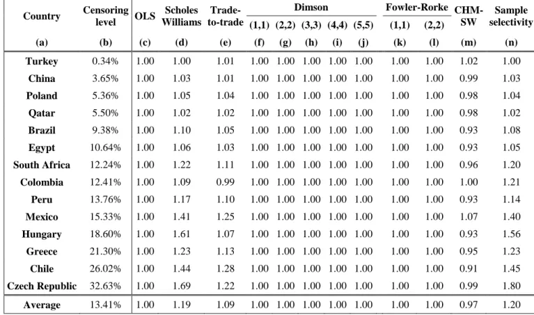
(34) 25. the last row of both tables, is computed as the simple average of the individual countries’ average betas. In theory, when an equally weighted index is used, as in Table 2a, the resulting average beta of the complete universe of stocks should equal one (Dimson, 1979). Such is the case for beta estimation methods like OLS, Dimson, and Fowler-Rorke, which have average betas of exactly one across all countries (columns c and f through l of Table 2a). CHMSW behaves similarly, with average betas very close to one for most countries (column m of Table 2a). With respect to the remaining adjustments, when the level of censoring is relatively low, as is the case for first few rows of Table 2a, the Scholes-Williams, trade-to-trade, and sample selectivity methodologies (columns d, e, and g, respectively) also have average betas close to one. However, as the censoring level increases, the equally weighted index begins to be dominated by thinly traded stocks and, as such, starts to suffer from thintrading problems itself. This introduces an upward bias in the resulting beta estimates for the adjustments that rely on trade-to-trade returns (Dimson, 1979). When a value weighted index is used, as in Table 2b, most average betas are substantially lower than 1, and there is no obvious pattern in beta behavior as a country’s level of censoring increases. However, the Scholes-Williams, trade-to-trade, and sample selectivity adjustments do result, for every country, in average betas that are greater than their OLS counterparts. This shows that the upward bias present when using an equally weighted index continues to exist, on average, when using a value weighted index. Another immediate observation from Tables 2a and 2b is that a value weighted index generally yields substantially lower beta estimates than an equally weighted index. This result is consistent with Brooks et al. (2007)..

(35) 26. Table 2a. Mean beta estimates by country using an equally weighted index. Country. Dimson Censoring Scholes TradeOLS level Williams to-trade (1,1) (2,2) (3,3) (4,4) (5,5). (a). (b). (c). (d). (e). Turkey. 0.34%. 1.00. 1.00. 1.01. China. 3.65%. 1.00. 1.03. Poland. 5.36%. 1.00. Qatar. 5.50%. Brazil. (f). (g). (h). (i). (j). Fowler-Rorke CHM- Sample SW selectivity (1,1) (2,2) (k). (l). (m). (n). 1.00 1.00 1.00 1.00 1.00. 1.00. 1.00. 1.02. 1.00. 1.01. 1.00 1.00 1.00 1.00 1.00. 1.00. 1.00. 0.99. 1.03. 1.05. 1.04. 1.00 1.00 1.00 1.00 1.00. 1.00. 1.00. 0.98. 1.04. 1.00. 1.02. 1.02. 1.00 1.00 1.00 1.00 1.00. 1.00. 1.00. 0.98. 1.02. 9.38%. 1.00. 1.10. 1.05. 1.00 1.00 1.00 1.00 1.00. 1.00. 1.00. 0.93. 1.08. Egypt. 10.64%. 1.00. 1.06. 1.03. 1.00 1.00 1.00 1.00 1.00. 1.00. 1.00. 0.93. 1.05. South Africa. 12.24%. 1.00. 1.22. 1.11. 1.00 1.00 1.00 1.00 1.00. 1.00. 1.00. 0.96. 1.20. Colombia. 12.41%. 1.00. 1.09. 0.99. 1.00 1.00 1.00 1.00 1.00. 1.00. 1.00. 1.00. 1.21. Peru. 13.76%. 1.00. 1.17. 1.10. 1.00 1.00 1.00 1.00 1.00. 1.00. 1.00. 0.93. 1.14. Mexico. 15.33%. 1.00. 1.41. 1.25. 1.00 1.00 1.00 1.00 1.00. 1.00. 1.00. 1.07. 1.40. Hungary. 18.60%. 1.00. 1.61. 1.07. 1.00 1.00 1.00 1.00 1.00. 1.00. 1.00. 0.93. 1.56. Greece. 21.30%. 1.00. 1.23. 1.13. 1.00 1.00 1.00 1.00 1.00. 1.00. 1.00. 0.95. 1.23. Chile. 26.02%. 1.00. 1.44. 1.28. 1.00 1.00 1.00 1.00 1.00. 1.00. 1.00. 0.91. 1.45. Czech Republic. 32.63%. 1.00. 1.69. 1.22. 1.00 1.00 1.00 1.00 1.00. 1.00. 1.00. 0.99. 1.80. Average. 13.41%. 1.00. 1.19. 1.09. 1.00 1.00 1.00 1.00 1.00. 1.00. 1.00. 0.97. 1.20. Table 2a shows mean beta estimates by country using an equally weighted index (columns c through n). The mean beta for each adjustment is computed. 26. as the simple average of all the betas of a given country’s stocks..

(36) 27. Table 2b. Mean beta estimates by country using a value weighted index. Country. Dimson Censoring Scholes TradeOLS level Williams to-trade (1,1) (2,2) (3,3) (4,4) (5,5). (a). (b). (c). (d). (e). Turkey. 0.34%. 0.79. 0.79. 0.80. China. 3.65%. 0.91. 0.91. Poland. 5.36%. 0.73. Qatar. 5.50%. Brazil. (f). (g). (h). (i). (j). Fowler-Rorke CHM- Sample SW selectivity (1,1) (2,2) (k). (l). (m). (n). 0.79 0.76 0.77 0.82 0.82. 0.79. 0.76. 0.74. 0.80. 0.91. 0.88 0.87 0.86 0.85 0.84. 0.88. 0.87. 0.87. 0.93. 0.78. 0.76. 0.74 0.75 0.82 0.83 0.87. 0.74. 0.74. 0.72. 0.76. 0.85. 0.90. 0.87. 0.88 0.88 0.93 0.87 0.85. 0.88. 0.87. 0.86. 0.88. 9.92%. 0.51. 0.62. 0.53. 0.59 0.64 0.68 0.69 0.75. 0.59. 0.64. 0.61. 0.54. Egypt. 10.64%. 1.04. 1.21. 1.07. 1.16 1.17 1.18 1.19 1.26. 1.14. 1.15. 1.12. 1.09. South Africa. 12.24%. 0.59. 0.72. 0.64. 0.64 0.66 0.70 0.70 0.75. 0.64. 0.66. 0.63. 0.66. Colombia. 12.41%. 0.73. 0.90. 0.77. 0.82 0.84 0.86 0.84 0.80. 0.81. 0.83. 0.81. 0.79. Peru. 13.76%. 0.70. 0.85. 0.78. 0.73 0.76 0.77 0.79 0.81. 0.73. 0.75. 0.71. 0.79. Mexico. 15.33%. 0.46. 0.59. 0.52. 0.51 0.48 0.53 0.54 0.49. 0.51. 0.48. 0.49. 0.52. Hungary. 18.60%. 0.39. 0.41. 0.44. 0.48 0.47 0.47 0.46 0.46. 0.42. 0.44. 0.47. 0.41. Greece. 21.30%. 0.52. 0.59. 0.57. 0.52 0.55 0.58 0.59 0.61. 0.52. 0.55. 0.51. 0.59. Chile. 26.02%. 0.64. 0.89. 0.76. 0.68 0.74 0.75 0.81 0.80. 0.67. 0.73. 0.66. 0.81. Czech Republic. 32.63%. 0.28. 0.69. 0.43. 0.46 0.51 0.58 0.63 0.68. 0.48. 0.54. 0.52. 0.42. Average. 13.41%. 0.65. 0.70. 0.70. 0.72 0.75 0.76 0.77 0.78. 0.69. 0.70. 0.72. 0.71. 27. Table 2b shows mean beta estimates by country using a value weighted index (columns c through n). The mean beta for each adjustment is computed as the simple average of all the betas of a given country’s stocks..

(37) 28. 5.2. Portfolios’ beta estimates. Using the linear programming model introduced in Section 3.1, we create five portfolios with equal risk characteristics but different levels of censoring for each emerging country. For almost every country, the model is able to form balanced portfolios, achieving equal mean and dispersion levels across all risk factors, as seen in Tables A.2.a and A.2.b of the Appendix, respectively. The exception is Turkey, for which the model could not create five distinct portfolios due to a very low level of censoring; Turkey is excluded from the below analyses. From Tables A.2.a and A.2.b, we see that, overall, the spread in censoring levels across portfolios is substantial (column c), confirming that the linear programming model is successful in the creation of portfolios that differ on this dimension. Meanwhile, all other factors (columns e through k), have approximately equal means (Table A.2.a) and degrees of dispersion (Table A.2.b) across portfolios. As stated in Section 3.1.2, we compute each portfolio beta as the weighted sum of its constituent stocks’ betas, where the weights are derived from the linear programming model. Tables A.3.a and A.3.b of the Appendix show the estimated betas by country and portfolio for equally weighted and value weighted indexes, respectively. The OLS beta decreases with portfolio censoring, evidencing the presence of thin trading bias, in line with the results presented by Bartholdy & Riding (1994) and McInish & Wood (1986), among others.21 In contrast, the adjustments tend to generate higher betas than the OLS method, correcting for the downward bias that arises from thin trading, especially when a portfolio’s level of censoring is relatively high. This occurs when both equally weighted and value weighed indexes are used.. 21. See also Jog & Riding (1986), Brooks et al. (2005), Davidson & Josev (2005), Iqbal & Brooks (2007),. and Hasnoui (2014)..

(38) 29. When comparing results from Tables A.3.a and A.3.b, we observe that risk estimates are substantially lower when a value weighted index is used. This result holds for most countries and beta estimates, including the OLS beta, and is in line with the findings of Brooks et al. (2007) and Corhay (1992). A value weighted index places more importance on larger firms’ returns; thus, when we estimate risk based on this index, the resulting beta tends to be lower (Iqbal & Brooks, 2007), as risk is inversely proportional to size (Frankfurter & Vertes, 1990).. 5.3. Comparison of adjustments against the OLS beta estimate. As discussed above, we posit that the method that best accounts for thin trading is that which gives the most similar results across portfolios for a given country. Therefore, we use a ranking metric that considers the difference between the maximum and minimum beta for each adjustment across the portfolios. Table 3 shows, for each beta adjustment and market index, the median spread between the maximum and minimum portfolio betas across all countries. By comparing the average spread for each beta adjustment with respect to the spread for the OLS method, we can establish the percentage of improvement over the OLS beta that each adjustment yields. For example, when an equally weighted index is used, the OLS betas yield a spread of 0.709 (column a). This spread decreases to 0.469 when we use the same equally weighted index and the Scholes-Williams adjustment, which translates to a 33.8% improvement (column b). When an equally weighted index is used, the median maximum-minimum spreads for all adjustments show improvement over the OLS method. The sample selectivity (column l) and trade-to-trade (column c) adjustments show the largest improvements: 40.9% and 34.9%, respectively. In contrast, the Fowler-Rorke adjustment (column j) with two leads and lags shows the poorest performance, with only a 3.7% enhancement over OLS. The conclusions are rather different if we study the results obtained using a value weighted index. The OLS estimate does not perform as poorly as in the previous case, and often.

(39) 30. outperforms the adjustment procedures. On average, the Dimson with five leads and lags (column h), sample selectivity (column l), and trade-to-trade (column c) adjustments continue to behave better than the OLS estimate, with 17.4%, 6.2%, and 6.0% improvement, respectively. In contrast, the Fowler-Rorke adjustment with one lead and lag (column i) shows the poorest performance: 18% worse than the OLS estimate..

(40) 31. Table 3. Median country spread between maximum and minimum beta estimates and percentage improvement over OLS beta. OLS Scholes- TradeWilliams to-trade (a). (b). (c). Dimson (1,1) (d). (2,2) (e). (3,3) (f). Fowler-Rorke CHM- Sample SW selectivity (4,4) (5,5) (1,1) (2,2) (g) (h) (i) (j) (k) (l). Equal weighted index Median max.-min. spread 0.709 0.469 % improvement over OLS 33.8%. 0.461 0.611 0.612 0.682 0.501 0.498 0.619 0.683 0.664 34.9% 13.8% 13.7% 3.8% 29.3% 29.7% 12.7% 3.7% 6.4%. 0.419 40.9%. Value weighted index Median max.-min. spread 0.382 % improvement over OLS. 0.359 0.442 0.390 0.424 0.414 0.316 0.451 0.433 0.384 6.0% -15.6% -2.1% -10.9% -8.2% 17.4% -18.0% -13.3% -0.4%. 0.358 6.2%. 0.398 -4.1%. Table 3 shows the median country spread between the maximum and minimum beta estimates for each portfolio and market index, and how this spread compares with that of the OLS method.. 31.

(41) 32. 5.4. Comparison of adjustments against each other. We next study how the beta adjustments behave with respect to each other. Tables 4a and 4b show, for each country (column a), how the different beta estimates rank (columns c through n). We rank the beta adjustments according to the portfolio spreads that they yield using a scale of 1 to 12: 1 for the adjustment that yields the lowest spread and 12 for the one that yields the highest spread. Thus, the best adjustments are those with lowest ranks. In Table 4a, for example, for Brazil, the sample selectivity adjustment (column n) shows the lowest spread, and thus is ranked 1, followed by the trade-to-trade (column e) and Scholes-Williams (column d) adjustments, ranked 2 and 3, respectively. The method that exhibits the highest spread in this country is the OLS method (column c), and therefore it is ranked 12. In Table 4a, when we use an equally weighted index, the OLS method (column c) ranks last or second to last in 7 out of the 13 countries. Moreover, it does not rank first for any of the countries. On average, the OLS beta seems to exhibit the poorest performance, with an average ranking of 9.7. This serves to show that the OLS method is subject to more thin trading bias than the adjustments. Meanwhile, the sample selectivity, ScholesWilliams, and trade-to-trade adjustments (columns d, e, and n, respectively) show the strongest results, with average rankings of 3.4, 4.1, and 4.9, respectively. These adjustments show the strongest results for all countries, with the exception of South Africa, Hungary, and the Czech Republic, where some specifications of Dimson’s or Fowler-Rorke’s adjustments appear to work better. In particular, for these latter countries, the Fowler-Rorke method with two leads and lags (column l) seems like a viable estimator. The adjustments that rely on leading and lagging market returns, as do the Dimson, Fowler-Rorke, and CHMSW adjustments, generally do not exhibit a clear pattern of performance across countries; they work well in some, and poorly in others. However, the Dimson adjustment, with its various leading and lagging specifications, seems to work, globally, better than the Fowler-Rorke and CHMSW techniques..

(42) 33. In Table 4b, when we compare the beta estimates based on a value weighted index, the results do not vary much; however, the OLS beta is no longer the worst ranking estimator. In this scenario, the OLS beta ranks last or second to last in only 3 out of the 13 countries; therefore, it does not perform as poorly as it did when an equally weighed index was used. We attribute this improvement to the fact that a value weighted index, by prioritizing larger, more liquid firms, suffers less from thin trading bias than an equally weighted index. Thus, using a value weighted index partially accounts for the bias that arises from thin trading.22 Even though the OLS estimate performs better when a value index is used, it is still outperformed by various adjustments. The sample selectivity, trade-to-trade, and ScholesWilliams adjustments (columns d, e, and n) continue to rank the highest, with rankings of 3.8, 4.4, and 4.5, respectively. With regards to the Dimson adjustment, the ranking for this method worsens as more leads and lags are introduced. With respect to the Fowler-Rorke adjustment, the specification with two leads and lags (column l) continues to work better than the version with one lad and lag (column k), similar to when an equally weighted index was used.. 22. In fact, in the Czech Republic, where the level of censoring is the highest, the best ranking estimate is the. OLS beta when a value weighted index was used..

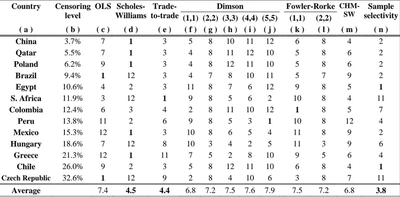
(43) 34. Table 4a. Beta rankings based on max-min portfolio spread, equally weighted index. Country. Censoring OLS Scholes- TradeDimson level Williams to-trade (1,1) (2,2) (3,3) (4,4) (a) (b) (c) (d) (e) (f) (g) (h) (i) 3.7% 7 4 5 9 10 11 China 1 5.5% 8 3 4 5 10 12 Qatar 1 6.2% 11 3 4 8 10 12 Poland 1 9.4% 12 3 2 7 8 6 5 Brazil 10.6% 12 11 5 9 7 4 Egypt 1 11.9% 9 12 10 8 5 4 S. Africa 1 12.4% 2 7 3 6 9 10 11 Colombia 13.8% 12 3 8 9 6 4 2 Peru 15.3% 12 2 3 10 7 6 5 Mexico 18.6% 5 11 4 6 2 3 8 Hungary 21.3% 12 2 4 10 7 3 5 Greece 26.0% 12 2 3 7 4 11 10 Chile Czech Republic 32.6% 3 11 10 8 4 5 1 Average. 9.7. 4.1. 4.9. 6.9. 6.4. 6.7. 6.8. (5,5) (j) 12 11 6 4 6 2 12 1 4 12 6 9 9 6.6. Fowler-Rorke CHM- Sample (1,1) (2,2) SW selectivity (k) (l) (m) (n) 6 8 2 3 6 7 9 2 5 9 7 2 10 9 11 1 8 10 3 2 7 3 6 11 4 8 5 1 10 7 11 5 11 9 8 1 7 9 10 1 11 8 9 1 8 6 5 1 7 2 6 12 7.9. 7.0. 7.5. 3.4. 34. Table 4a shows how the OLS beta and the different beta adjustments compare when using an equally weighted index. We rank each beta adjustment according to the spread between the portfolios with the largest and smallest beta within each country. We assign a rank of 1 to the method that yields the lowest spread, and 12 to that which yields the largest spread. The top-ranked method for each country and the three top-ranked methods overall are bolded..

(44) 35. Table 4b. Beta ranking based on max-min portfolio spread, value weighted index. Country. Censoring OLS Scholes- TradeDimson level Williams to-trade (1,1) (2,2) (3,3) (4,4) (a) (b) (c) (d) (e) (f) (g) (h) (i) 3.7% 7 3 5 8 10 11 China 1 5.5% 7 3 4 8 11 12 Qatar 1 6.2% 9 3 4 8 12 11 Poland 1 9.4% 12 3 4 7 8 10 Brazil 1 10.6% 4 2 3 11 8 7 6 Egypt 11.9% 3 12 9 8 5 6 S. Africa 1 12.4% 6 3 4 2 8 11 10 Colombia 13.8% 11 2 6 9 8 5 3 Peru 15.3% 12 3 10 8 6 5 Mexico 1 18.6% 7 12 8 10 3 4 2 Hungary 21.3% 12 11 7 5 2 8 Greece 1 26.0% 9 2 3 5 8 12 11 Chile Czech Republic 32.6% 12 9 2 8 4 10 1 Average. 7.4. 4.5. 4.4. 6.8. 7.2. 7.5. 7.6. (5,5) (j) 12 10 10 11 12 2 12 1 4 5 10 10 6 7.9. Fowler-Rorke CHM- Sample (1,1) (2,2) SW selectivity (k) (l) (m) (n) 6 8 4 2 5 8 6 2 5 8 6 2 5 7 9 2 9 8 5 1 10 8 4 11 8 5 7 1 10 8 12 4 11 8 9 2 11 3 9 6 9 5 6 4 6 8 4 1 3 8 7 11 7.5. 7.2. 6.8. 3.8. 35. Table 4b shows how the OLS beta and the different beta adjustments compare when using a value weighted index. We rank each beta adjustment according to the spread between the portfolios with the largest and smallest beta within each country. We assign a rank of 1 to the method that yields the lowest spread, and 12 to that which yields the largest spread. The top-ranked method for each country and the three top-ranked methods overall are bolded..

(45) 36. 6.. Conclusion. We compare a variety of beta adjustment techniques proposed in the literature to deal with the presence of thin trading bias in a significant, complete, and independently defined group of emerging markets. We form portfolios with equal risk factors, but different levels of censoring, through the use of a linear programming model. The formation of such portfolios allows us to create a basis of comparison between the beta adjustments. Because beta is a measure of systematic risk, if most risk factors are kept constant across portfolios, the resulting betas should be approximately the same. Therefore, the best adjustment is that which yields the most similar betas across portfolios. The main findings of our study are the following. First, we corroborate that beta estimates obtained using an equally weighted index are substantially higher than those obtained using a value weighted index. Second, we find that the beta adjustments generally outperform the standard OLS estimate when we use an equally weighted index. Moreover, the sample selectivity and trade-to-trade adjustments yield the best results, showing 40.9% and 34.9% less bias than OLS betas, respectively. On the other hand, when a value weighted index is used, the OLS beta is no longer outperformed by all the adjustments, and seems to perform much better overall. We attribute this improvement to the fact that value weighted indexes, due to their more liquid nature, partially correct for thin trading bias. Third, when the adjustments are compared between each other, we find that betas that compute returns on a trade-to-trade basis – namely, the sample selectivity, ScholesWilliams, and trade-to-trade betas – show the best results for both equally weighted and value weighted indexes. In fact, for over 60% of the emerging markets under study, the sample selectivity adjustment ranks first or second when an equally weighted index is used. Similarly, for over 50% of these countries, it ranks first or second when a value weighted index is used..