Analysis of energy data of existing buildings in a University Campus
11
0
0
Texto completo
(2) In general, the service sector, which includes university campuses, has been expanding continuously for the last decades and as a result, the energy consumption of this sector has also grown. In fact, according to the International Energy Agency (IEA), the electricity use of service sector represented a global share of 50% worldwide electricity consumption in 2011 and it increased by nearly 56% between 1990 and 2011 (International Energy Agency, 2015). This reflects the growing importance of electricity-consuming artefacts and the role they have been playing, such as in office equipment, information and communication technologies (ICTs) in addition to lighting and air conditioning. Therefore, the management and control of energy consumption with the aim of increasing the energy efficiency of buildings has turned into a global necessity and a viable option for combating climate change in the short term. During the 1990s, information technology (IT) tools capable of analysing information obtained from consumption sensors of buildings have emerged with the objective of improving the management of the energy resources of the commercial and industrial sector. These tools permit validating monthly electricity bills, analysing patterns of use in relation to building type, and verifying the behaviour of consumption in the face of changes of equipment and their impact on consumption (Younger, 2007). In the way a purely statistical analysis is useful when the relationship between the variables to be analysed is well defined, the strength of this relationship can also be shown in the same way. However, if the analyst does not know what results are likely to be obtained from the data, it is more appropriate to show this information graphically in order to effectively establish possible relationships (Abbas & Haberl, 1994). Several studies have put forward graphic representations of large amounts of energy consumption data in order to permit the user to analyse them and take decisions based thereupon. In 1994, graphic indices were used to analyse between 20,000 and 30,000 hours of energy consumption obtained from LoanSTAR, a revolving loan programme financing energy-related cost-reduction retrofits for public buildings and similar facilities in Texas (Abbas & Haberl, 1994). The use of graphs to show information about the energy consumption of buildings turns out to be more efficient and easier to understand by the user than statistical analysis. Energy consumption data is usually represented in the form of bar graphs (Ahmed, Ploennigs, Gao, & Menzel, 2009; Buchmann, Böhm, Burghardt, & Kessler, 2013), time series (Younger, 2007), and scatter diagrams (Reddy, 2006); other techniques include box whisker mean plots (BWM) and carpet plots (Raftery & Keane, 2011). The more advanced techniques are those applied by virtue of using ‘data mining’ to reduce dimensionality and to allow carrying out projections of continuous maps by interpolation of discrete variables (Morán, 2012). Several case studies analysing the energy consumption in buildings of university campuses in order to improve the its management and to establish relationships between consumption and variables such as occupancy, use and outdoor temperature have been published (Deng, Dai, Wang, & Zhai, 2011; Gul & Patidar, 2015; Morán, 2012; Valderrama, Cohen, Lagiere, & Puiggali, 2011; Wong, Fellows &, Liu, 2006). In 2006, a case study of the University of Hong-Kong demonstrated that seasonal climate was the variable with the greatest impact on the monthly consumption profile in buildings with a heating, ventilation and air conditioning (HVAC) system using annual time series. In addition, the study showed a significant relation between different consumption patterns, and occupancy and use of the building (Wong et al., 2006). A previous analytical study of energy consumption at the University of Bordeaux also found that the climate variable, in particular outdoor temperature and heating degree-days (HDDs), was the most important factor influencing energy consumption as opposed to relative humidity and wind speed, which were more related to the feeling of comfort of the user (Valderrama et al., 2011). HDDs are defined as the cumulative deficit of temperature from a reference temperature over time (CIBSE, 2006). The reference temperature known as base temperature is usually standardized at national level. (Azevedo, Chapman, & Muller, 2015) show the relationship between electric consumption of Birmingham, UK and HDDs and cooling degree days (CDDs). The authors highlight the importance of choosing the right base temperatures for HDDs and CDDs calculation. The focus of this investigation, different from the studies cited, which are concentrated either on one building or on general data including the total consumption of the campus, is to analyse the electricity consumption of each building on campus and compare the consumption between buildings over the time of the study, and by trying to take advantage of hourly interval data in a simple form by the use of graphic representations.. Methodology An analysis of energy consumption data is essential for obtaining the feedback necessary to control the available energy resources, and in order to carry out this process as efficiently as possible, the use of resources (time, money) needed 173.
(3) for the analysis should to be kept to a minimum. The objective of the proposed method is to make it possible to obtain clear and above all easy-to-understand information for taking decisions as far as the management of energy is concerned. In addition, the method permits analysing the data of one or more buildings and comparing them among each other according to consumption based on surface and use. Obtaining the consumption data The data are to be extracted from the storage server that contains the cumulative consumption that a meter registers every hour, and then the difference between contiguous records is to be calculated so that the hourly consumption data can be obtained, with which the analysis is to be carried out. In order to make sure that the energy data are reliable, Buildings with the best data representation are selected as to assure that the conclusions to be drawn can be seen as correct. As has already been seen in previous studies, in order to generate profiles of consumption, the data are to be grouped into three sets, i.e. of working days, Saturdays, and Sundays and holidays (Jalori & Reddy, 2015; Morán, 2012). Determination of characteristics In order to carry out the analysis, the building from which the data come – the type of building, its use, and its useable area – is to be identified. In addition, information about the environmental variables for the correlation, in this case the outdoor temperature, is to be obtained. To include the variable of outdoor temperature the HDD need to be calculated, for which the following expression is used (Azevedo et al., 2015). 𝑇𝑚𝑖𝑛,𝑑𝑎𝑦 + 𝑇𝑚𝑖𝑛,𝑑𝑎𝑦 𝐻𝐷𝐷 = ∑ ( − 𝑇𝑏𝑎𝑠𝑒 > 0) 2 where Tmin represents the minimum daily temperature recorded in degrees Celsius, T max the maximum temperature in degrees Celsius, and Tbase is the base reference temperature for the calculation, whose value corresponds to the outdoor temperature at which air conditioning in the building is not needed. HDDs can be calculated on yearly, monthly or daily period (Amber et al., 2018). Data comparison In order to compare the consumption between buildings, the hourly consumption values are divided by the maximum value of all the buildings, obtaining values between 0 and 1, which allows for distinguishing the buildings that consume more energy and where control measures are likely to have a greater impact. It also permits identifying similar consumption profiles between buildings according to building type (Valderrama et al., 2011). Data projection Graphs are produced containing the information of each building, either separately or in comparison. Time series plots and bar charts show the consumption of the building or buildings in order to identify and analyse the intervals of the electricity consumption. BWM plots are used to represent the daily consumption profiles of each building. In addition, scatter diagrams illustrating the relation between HDDs and electricity consumption of a building are considered.. Results and discussion The data of electricity consumption used in this study were those of buildings belonging to the Science and Technology campus of the University of Bordeaux located in Talence in France. The time frame covering the study was affected by the project ‘Opération Campus’, which aimed at optimising and rationalising the work areas of the university community. The project had already concluded its first stage, which involved renovating part of the campus, and was handed over in February 2016 after two years of work. This renovation meant changes to the infrastructure of the buildings pertaining to the 1960s and 70s so that they complied with the standards of sustainability and comfort required by the current French building regulations (Université de Bordeaux, 2016). Description of the collection of buildings A group of thirty buildings are to be analysed, which amount to a total of 147,430 m2 of constructed surface. The buildings can be grouped according to their use into buildings for teaching, research, administration and mixed purposes. In turn, the constructed surface for teaching purposes (T) corresponds to 55,685 m2 and is composed of 174.
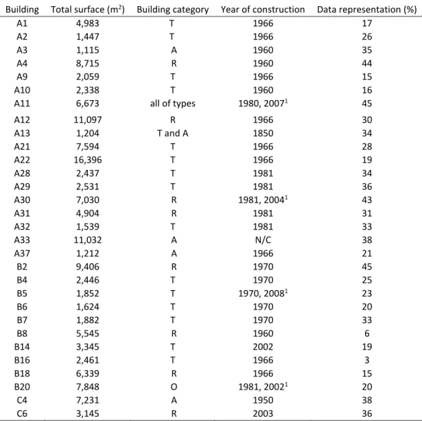
(4) classrooms and lecture theatres, that of research (R) amounts to 60,605 m 2 corresponding to laboratories and offices. Finally, 22,208 m2 pertain to the administration of the campus and academic units (A), and 8,932 m2 belong to the category of ‘other’ (O), representing libraries and the Institute of Optics ALPHANOV. The details of each building are listed in Table 1. Table 1 shows the data representation which is the ratio of hours with available energy data to the total number of hours over the three-year period. For space heating, all buildings are connected to a district heating distribution system using biomass and natural gas as energy sources. Therefore, lighting and electrical appliance should drive electric loads. The campus is open all day on working days (from Monday to Friday) and half the day on Saturdays. It is closed on Sundays and holydays. Table 1. Results of information gathered about the buildings. Source: Self-Elaboration.. Building A1 A2 A3 A4 A9 A10 A11. Total surface (m2) 4,983 1,447 1,115 8,715 2,059 2,338 6,673. Building category T T A R T T all of types. Year of construction 1966 1966 1960 1960 1966 1960 1980, 20071. Data representation (%) 17 26 35 44 15 16 45. A12 A13 A21 A22 A28 A29 A30 A31 A32 A33 A37 B2 B4 B5 B6 B7 B8 B14 B16 B18 B20 C4 C6. 11,097 1,204 7,594 16,396 2,437 2,531 7,030 4,904 1,539 11,032 1,212 9,406 2,446 1,852 1,624 1,882 5,545 3,345 2,461 6,339 7,848 7,231 3,145. R T and A T T T T R R T A A R T T T T R T T R O A R. 1966 1850 1966 1966 1981 1981 1981, 20041 1981 1981 N/C 1966 1970 1970 1970, 20081 1970 1970 1960 2002 1966 1966 1981, 20021 1950 2003. 30 34 28 19 34 36 43 31 33 38 21 45 25 23 20 33 6 19 3 15 20 38 36. 1Building. extensions or some other structural modification.. Meteorological variable With the meteorological information provided by the city of Bordeaux from 2013 to 2016, the HDD were calculated for the purpose of relating the consumption behaviour of the buildings to this variable. In addition, the monthly HDD were calculated as the sum of the HDD for each month representing the climate of Bordeaux. The base temperature T was considered to be 18°C as usually used in France. base. As can be seen in Figure 2, the months of December, January, February, and to a lesser extent March and November, present the greatest values of HDD when heating the buildings is required and therefore, greater consumption by the heating system is expected during those months. It should be pointed out that the time of year when heating is needed, 175.
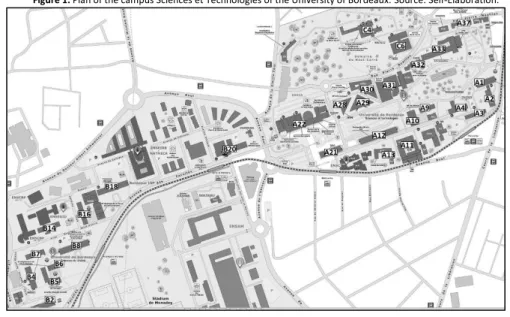
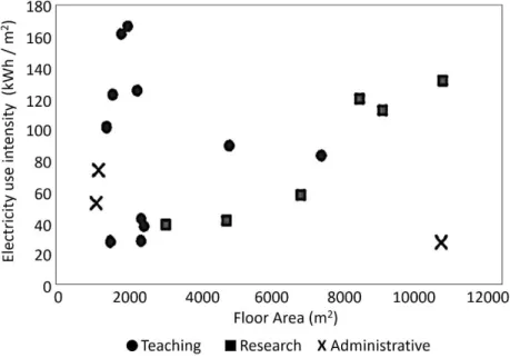
(5) corresponds to the academic period, which directly influences the occupancy of the buildings and their consumption. Even though during the months from June to September air conditioning is required in the buildings, these months correspond to the lowest occupancy on account of it coinciding with the exam and holiday period. Figure 1. Plan of the campus Sciences et Technologies of the University of Bordeaux. Source: Self-Elaboration.. Figure 2. Average monthly heating degree-days (HDDs) from 1991 to 2010. Source: Self-Elaboration.. Availability and quality of the consumption data The electricity consumption data used for the study span from 14 January 2013 to 6 May 2016. However, not all the data can be accounted for during this period, presumably due to problems with the recording system. In addition, with regard to the quality of the available data, it was necessary to carry out an exhaustive review and validation of the data in order to eliminate erroneous data and/or those that were incorrectly recorded. The data representation varied between buildings, which in the best case reached 45% and the worst case reached 3%. However, it was observed that the missing data correspond largely to the academic summer and holiday period, placing the available data between the months of October and May, during which period the campus is at its most active, thus covering the most useful period with regard to the analysis to be carried out. Analysis of electricity consumption In Figure 3, a collection of twenty buildings is shown by means of a scatter plot, in which each series represents a type of building, for either teaching (T), research (R) or administration (A) (see Table 1). The plot shows the electricity use intensity as the annual consumption of each building per square meters in relation to its surface area. The plot shows the electricity use intensity (EUI) of the twenty buildings in 2013. The objective of this representation is to illustrate the consumption of the respective types of buildings and to show how the consumption behaves in relation to the total surface area of the buildings. 176.
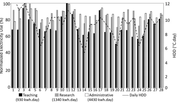
(6) Figure 3. Electricity use intensity in relation to the total surface area of the building in 2013. Source: Self-elaboration.. From the plot it can be elicited that the majority of the buildings dedicated to teaching have between 1,000 m2 and 2,500 m2 of constructed surface. The two teaching buildings that have a greater surface are A1 and A21 with areas of 4,983 m2 and 7,594 m2, respectively. With regard to the ratios of consumption to surface they range between 27 and 166 kWh/m2 in the case of the teaching buildings. This can be attributed to the fact that the consumption of these buildings, which largely consist of lecture theatres, depends to a great extent on their occupancy and the occupancy rate of classrooms, given that some buildings are in greater demand than others. As an example, the building representing the greatest consumption is A9 with an area of 2,059 m 2, which consumes six times more than that with the lowest consumption (A32 with 1,539 m2). Another factor to which the spread of the consumption among the teaching buildings can be attributed is the year of construction. It was found that the buildings with the lowest were built in 1981 while those with the highest EUI were constructed between the 1960s and 70s because the more recent buildings have better standards of design and construction regarding natural light and thermal insulation as well as, presumably, more efficient systems. The surface areas of the research buildings range from 3,145 m 2 to 11,097 m2. Depending on the area of research that is being conducted, a different amount of space will be needed for laboratories, offices and equipment. These buildings present a EUI that increases proportionally as the total built surface area increases and ranges from 38 kWh/m 2 for the lowest to 131 kWh/m2 for the highest ratio. Although the buildings with a higher ratio tend to be older (between 10 and 30 years), this variable is insignificant if one considers that the consumption corresponds primarily to the activities carried out in the specific laboratory; furthermore, it can be assumed that the installations and the necessary equipment for the respective research tasks are responsible for the consumption. Finally, the administrative buildings have an EUI between 26 and 74 kWh/m2, which represents a much narrower and more homogeneous range than that of the teaching and the research buildings. In Figure 4 the data of three buildings, administration, research, and teaching, corresponding to February 2014 can be seen. The chart illustrates the normalised daily consumption in relation to the maximum value of each building in the considered month, and the HDD corresponding to the specific day, shown by the broken line. The purpose of the chart is to compare the consumption of the buildings between each other as well as their behaviour between the different days of the week within the same month. In addition, it allows linking the consumption to the HDD. It can be seen that the HDD have a significant impact on the consumption of the buildings since it follows approximately the same trend, i.e. on higher HDD the consumption is higher while on lower HDD the total consumption also appears to be lower. This relation is more pronounced in the administrative-type building than in those for research and teaching, which can be attributed to the fact that the consumption of the administrative building is shown to be more homogeneous. As was to be expected, the days of the weekend show a lower consumption than the working days especially for research and administrative buildings, which can be seen in the Figure.. 177.
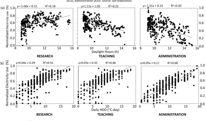
(7) Figure 4. Comparison of normalized consumption between building type. Source: Self elaboration.. Grouping the consumption of the buildings into working days, Saturdays, Sundays and holidays over the three-year period allows for a more exact analysis of the differences in the behaviour expected and the true behaviour between the types of days. In addition, it permits identifying a better potential for the energy use of the heating or air conditioning system of the building. By plotting the daily consumption against the meteorological variable of HDD, producing a scatter plot, the relationship between the latter variable and the electricity consumption of the administrative building A33 could be determined as is shown in Figure 5. In Figure 5a it can be seen that the R 2 value for the working days, amounting to 0.73, indicates some interdependence between the electricity consumption and the HDDs. On the other hand, regarding Saturdays when the activity in the building is minimal and limited to half a day, the relationship between these variables is considerably less strong, which is reflected in the R2 value of 0.45 (Figure 5b). In the case of Sundays, when no activity in the building is expected and its occupancy is estimated to be nil, the correlation decreases (Figure 5c) still further (R2 = 0.40) on account of the large spread of the data points . The correlation coefficients of Saturdays and Sundays were found to be closer to what was to be expected. Therefore, it became necessary to carry out the analyses of Sundays and holidays separately. In the latter case, the correlation appears to be the strongest given R 2 = 0.79 (Figure 5d). Figure 5. Electricity consumption of Building A33 (adm) related to HDD grouped by days. Source: Self elaboration.. In Figure 6, the normalised consumption versus HDD is shown of a research, a teaching and an administrative building with correlation coefficients of R2 = 0.602, 0.409 and 0.731, respectively. These values demonstrate that the HDD influence the consumption differently depending on the type of building and its use. The administrative-type building has the highest correlation coefficient due to the variability of its consumption depending to a great extent on the outdoor temperature. The research building presents a similar correlation coefficient to that of the administrative building, which can be explained by the fact that its consumption is also relatively homogeneous during the year. Lastly, the teaching building has the lowest correlation coefficient, which is thought to be as a result of its consumption depending largely on the variable of occupancy.. 178.
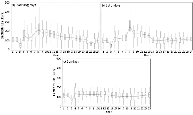
(8) Figure 6. Normalised energy consumption versus a) daylight length and b) Daily HDD by type of building: Research (A11), Teaching (A13), Administration (A33). Source: Self elaboration.. Consumption profiles Figures 7 and 8 show the consumption profiles by way of BWM plots, where the data are divided into quartiles – the box containing 50% of the data while the whiskers represent the upper and lower 25% of the data; the line connects the medians of the consumption. Separate profiles were generated for working days, Saturdays and Sundays. This type of representation helps to understand the dynamics of the consumption of the building by showing the distribution of the hourly consumption over a determined space of time, in this case the periods autumn and winter of 2013-2016. In Figure 7a it can be seen that the consumption on working days (from Monday to Friday) reaches a peak at 08:00 hrs and subsequently decreases gradually during the course of the day. This peak observed on administrative buildings electric load profiles and not on teaching buildings electric load profiles can be attributed to individual electric heating of offices. The use of individual heating points out the deficiency of central heating system or its control to meet user’s thermal comfort. Considering the Saturday profile (Figure 7b), it also reaches a peak at 08:00 hrs but on this occasion it is much more pronounced. Between 09:00 hrs and 13:00 hrs the consumption behaves similarly to that on working days during the same time period but amounts to around 10% less. At 14:00 hrs end of the work day, the electric loads decreases until the baseline. On Sundays (Figure 7c) the consumption is relatively homogeneous throughout the day ranging between 100 and 150 kWh, which is to be expected owing to the fact that on those days the building is unoccupied. It should be pointed out that the time of the lowest consumption (03:00 hrs) is independent of the day. Furthermore, an hour later, at 04:00 hrs, a considerable increase in consumption has been observed in all cases.. 179.
(9) Figure 7. Electrical load profiles of the administrative buildings. Source: Self-elaboration.. Figure 8 illustrates the consumption profiles for a teaching building. On working days, the consumption increases at 07:00 hrs and remains constant until 11:00 hrs; thereafter it decreases and remains flat from 14:00 hrs until 23:00 hrs. At 24:00 hrs another slight decrease in consumption is observed, which is maintained until 06:00 hrs. The behaviour on Saturdays is fairly similar to that on working days following the same trend except for a significant dip at 20:00 hrs. As was to be expected, on Sundays the consumption is homogeneous and somewhat lower than on the other days, however, observing a slight increase in the late evening. Figure 8. Electrical load profiles of the teaching buildings. Source: Self –elaboration.. Conclusions This work presents a simple analysis of the monitoring of the electricity consumption of a group of buildings in a university campus. The main aim of the analysis is to be able to compare a group of buildings among each other in such 180.
(10) a way as to determine which one, or which ones, control measures should focus on in order to allow for a more efficient energy management. The method also permits establishing the strength of the relationship between the outside temperature measured in heating degree days (HDD), daylight length and the electricity consumption of the different types of buildings in a university campus. In order to carry out the analysis, information about the buildings was gathered, including constructed surface, year of construction, their use (teaching, research, administration or mixed), and the amount of electricity consumed per hour/day/year, that was considered useful for representing the consumption of the buildings and essential for performing a conclusive analysis. Graphs used for the analysis include a scatter plot of the ratio of consumption to surface in relation to the surface area of the building, which allows for establishing the behaviour of the different types of buildings (administration, teaching and research) according to the constructed surface area. The time series graph of the daily electricity consumption, allows comparing the types of buildings between each other to determine which ones consume the most electricity as well as representing the behaviour of the consumption on the different days of the week. The HDD are also shown in the graph in order to analyse their trend and compare it with the consumption. To analyse the relation that exists between the consumption and the external temperature, a scatter plot is used showing the strength of correlation of the latter variable with the power consumed; in this case, separate graphs have to be produced for working days, Saturdays, Sundays and holidays so that the variable of occupancy can be added indirectly to the analysis. Lastly, box and whisker plots are used to generate the 24-hour consumption profiles, which allow visualising the changes in consumption over a day in detail and so find out what the consumption peaks are due to. It could be concluded that the teaching buildings in the campus have a varied ratio of consumption to surface and for this reason, an estimate of the electricity demand of these buildings should include the variable of occupancy through an indicator that takes into account the number of students using the building and the time they spend in it. The administrative buildings have a somewhat similar ratio although the older buildings have a higher ratio than the newer ones. The research buildings have a ratio that increases as its total surface area increases, which can be attributed to the fact that in buildings with a larger surface area activities requiring a greater use of electricity take place than in smaller buildings. The administrative buildings have a constant occupancy depending on the type of day, i.e. whether it is a working day, a Saturday or a Sunday. Therefore, by separating the analysis into one for each of these types of days, it could be shown that the external temperature was the most important variable with regard to consumption in the short term as well as in the long term. The buildings with the weakest correlation between consumption and HDD were those for teaching reaffirming the need to include the variable of occupancy in these buildings. In future research work, this method will be improved and applied to a Latin American university campus which have installed electricity meter in each buildings and have a political plan for improving sustainability of its constructed heritage.. References Abbas, M., & Haberl, J. (1994). Development of graphical indices for displaying large scale building energy data sets. Retrieved from http://repository.tamu.edu/bitstream/handle/1969.1/6642/ESL-HH-94-0523.pdf?sequence=4%255Cnhttp://repository.tamu.edu/handle/1969.1/6642 Ahmed, A., Ploennigs, J., Gao, Y., & Menzel, K. (2009). Analyse building performance data for energy-efficient building operation. In CIB W78 - 26th International Conference on Managing IT in Construction (pp. 211–220). Amber, K., Aslam, M., Ikram, F., Kousar, A., Ali, H., Akram, N., … Mushtaq, H. (2018). Heating and Cooling Degree-Days Maps of Pakistan. Energies, 11(1), 94. https://doi.org/10.3390/en11010094 Azevedo, J. A., Chapman, L., & Muller, C. L. (2015). Critique and suggested modifications of the degree days methodology to enable long-term electricity consumption assessments: a case study in Birmingham, UK. Meteorological Applications, 22(4), 789–796. https://doi.org/10.1002/met.1525 Buchmann, E., Böhm, K., Burghardt, T., & Kessler, S. (2013). Re-identification of Smart Meter data. Personal and Ubiquitous Computing, 17(4), 653– 662. https://doi.org/10.1007/s00779-012-0513-6 CIBSE. (2006). TM41 Degree-days: theory and application. (CIBSE Publications, Ed.). London: The Chatered Institution of Building Services Engineers. Deng, S., Dai, Y. J., Wang, R. Z., & Zhai, X. Q. (2011). Case study of green energy system design for a multi-function bulding in campus. Sustanaible Cities and Society, 152–163. https://doi.org/10.1016/j-scs.2011.07.002 European Climate Foundation (ECF), World Energy Council (WEC), Cambridge Judge Business School (CJBS), & Cambridge Institute for Sustainability Leadership (CISL). (2014). Cambio Climático : Implicaciones para el Sector Energético. Hallazgos claves del Quinto Informe de Evaluación (AR5) del Grupo Intergubernamental de Expertos sobre el Cambio Climático.. 181.
(11) Gul, M. S., & Patidar, S. (2015). Understanding the energy consumption and occupancy of a multi-purpose academic building. Energy and Buildings, 87, 155–165. https://doi.org/10.1016/j.enbuild.2014.11.027 International Energy Agency. (2015). Energy Efficiency Indicators: Essentials for Policy Making. Paris, France. Retrieved from https://www.iea.org/publications/freepublications/publication/IEA_EnergyEfficiencyIndicators_EssentialsforPolicyMaking.pdf Jalori, S., & Reddy, T. A. (2015). A new clustering method to identify outliers and diurnal schedules from building energy interval data. ASHRAE Transactions, 121, 33–44. Morán, A. (2012). Análisis y predicción de perfiles de consumo energético en edificios públicos mediante técnicas de minería de datos. Universidad de Oviedo. Porritt, J. (2005). Healthy environment—healthy people: The links between sustainable development and health. Public Health, 119(11), 952–953. https://doi.org/10.1016/j.puhe.2005.08.004 Raftery, P., & Keane, M. (2011). Visualizing patterns in building performance data. In Proceedings of Building Simulation 2011: 12th Conference of International Building Performance Simulation Association (pp. 9–15). Sidney: IBPSA nternational Building Performance Simulation Association. Reddy, T. A. (2006). Literature Review on Calibration of Building Energy Simulation Programs. ASHRAE Transactions, 112(1), 226–240. Retrieved from https://lt.ltag.bibl.liu.se/ Université de Bordeaux. (2016). OPÉRATION CAMPUS Bordeaux. Retrieved November 24, 2016, from https://operation-campus.u-bordeaux.fr Valderrama, C., Cohen, A., Lagiere, P., & Puiggali, J. R. (2011). Análisis del comportamiento energético en un conjunto de edificios multifuncionales. Caso de estudio Campus Universitario. Revista de La Construccion, 10(2), 26–39. https://doi.org/http://dx.doi.org/10.4067/S0718915X2011000200004 W.P. Wong, R.F. Fellows &, & A.M.M Liu. (2006). Use of Electrical Energy in University Building: a Hong Kong Case Study. Facilities, 24(1), 5–17. https://doi.org/10.1108/02632770610639161 Younger, W. (2007). Using interval meter data for improved https://doi.org/http://dx.doi.org/10.1080/01998590709509509. facility. management.. Energy. Engineering,. 104,. 21–32.. 182.
(12)
Figure
+3
Documento similar