Effects of electricity dynamic pricing : from time of use to real time pricing

Texto completo

(1)PONTIFICIA UNIVERSIDAD CATOLICA DE CHILE ESCUELA DE INGENIERIA. EFFECTS OF ELECTRICITY DYNAMIC PRICING: FROM TIME OF USE TO REAL TIME PRICING. RODRIGO ANDRÉS PEREZ ODEH. Thesis submitted to the Office of Research and Graduate Studies in partial fulfillment of the requirements for the Degree of Master of Science in Engineering Advisor: DAVID WATTS CASIMIS. Santiago de Chile, January, 2014  2014, Rodrigo Pérez Odeh.

(2) PONTIFICIA UNIVERSIDAD CATOLICA DE CHILE ESCUELA DE INGENIERIA. EFFECTS OF ELECTRICITY DYNAMIC PRICING: FROM TIME OF USE TO REAL TIME PRICING. RODRIGO ANDRÉS PEREZ ODEH. Members of the Committee: DAVID WATTS CASIMIS HUGH RUDNICK VAN DE WYNGARD YARELA FLORES AREVALO PATRICIO DEL SOL GUZMAN. Thesis submitted to the Office of Research and Graduate Studies in partial fulfillment of the requirements for the Degree of Master of Science in Engineering Santiago de Chile, January, 2014. ii.

(3) (A mi familia). iii.

(4) ACKNOWLEDGEMENTS First, I would like to thank my family, including my parents, brother and sister, grandparents and uncles for all their advices, support and contention. I would also like to thank my advisor Dr. David Watts, for his guiding and for the confidence he placed in me during this and other researches. My thanks are also extended to my friends for their advices and willingness to help. Finally, I want to remember my great-aunt.. iv.

(5) TABLE OF CONTENTS. ACKNOWLEDGEMENTS ........................................................................................ iv LIST OF FIGURES .................................................................................................... vii LIST OF TABLES ...................................................................................................... ix ABASTRACT .............................................................................................................. x RESUMEN .................................................................................................................. xi I.. INTRODUCTION .............................................................................................. 1 Energy demand and the need for infrastructure ............................................... 1 Demand could add value to electricity markets ............................................... 1 Incentive-based programs................................................................................. 2 Price-based programs ....................................................................................... 2. II.. PENNSYLVANIA-NEW JERSEYMARYLAND ELECTRICITY MARKET AND DESCRIPTION OF DATA ..................................................... 7 PJM demand description .................................................................................. 8 PJM supply description .................................................................................... 9. III.. ECONOMIC MODEL ...................................................................................... 12 Electricity demand function ........................................................................... 12 Electricity supply function ............................................................................. 13. IV. Rates applied to the model ................................................................................. 19 TOU: number of prices levels ........................................................................ 19 TOU: hours of the day where each price level is applied .............................. 19 TOU: magnitude of each price level .............................................................. 21 TOU2 – CPP rate ............................................................................................ 22 RTP rate .......................................................................................................... 24 V.. NUMERICAL RESULTS ................................................................................ 25 Peak reduction ................................................................................................ 26 v.

(6) Energy Consumption .................................................................................... 27 Consumer expense .......................................................................................... 28 VI.. CONCLUSIONS AND DISCUSSION ............................................................ 30. REFERENCES ........................................................................................................... 33. vi.

(7) LIST OF FIGURES Figure 1: Types of demand response programs (adapted from Dupont et al (2011) [8]) .............................................................................................................................. 4 Figure 2: Energy consumption (GWh) and Peak power demand (GW) in PJM at 2010. In summer months (June to September) consumption and monthly peak demand increased respect to the rest of the year. ....................................................... 8 Figure 3: Average daily load curve in summer months (June to September) and the rest of the year (October to May) are very different. ................................................. 9 Figure 4: Monthly average price and peak price for PJM at 2010. Prices shows the same seasonality behavior as the demand ................................................................ 11 Figure 5: Example of demand curve used for hour “h”. The term. is different. for every hour of the year to capture hourly and seasonal effects of the demand .... 13 Figure 6: Three different ToU rates with different demand functions and new equilibriums points ................................................................................................... 14 Figure 7: Case (a) Fixed supply with demand shifting in time (left) cause that equilibrium points map the supply curve, and - Case (b) fixed demand and supply shifting in time (right) cause that equilibrium points map the demand curve.......... 15 Figure 8: Capacity demand (MW) vs. temperature (°C) showing the positive correlation between temperature and demand in summer month (June to September) and the negative correlation in other month (December to March) ......................... 16 Figure 9: Average duration curve for summer month (June to September) segmented to identify the hours of each time block in a day. .................................. 20 Figure 10: Example of the blocks time in a day with ToU of 2,3 and 5 price levels21 Figure 11: ToU prices affect wholesale prices through a change in the demand..... 21 Figure 12:ToU of two price levels with different prices for each period. ToU rate vary according to the price elasticity "e". ................................................................ 22 Figure 13: Critical events in PJM 2010 interconnection. The first 5 critical events occurred in July at 5 pm ........................................................................................... 24 vii.

(8) Figure 14: Peak reduction (%) per type of rate and elasticity respect to flat rate .... 27 Figure 15: Consumption increase (%) per type of rate and elasticity respect to flat rate ........................................................................................................................... 28 Figure 16: Average consumer expense saved (%) per type of rate and elasticity .... 29. viii.

(9) LIST OF TABLES Table 1: S Airport codes used to retrieve temperature data from Wunderground website[22] and total population by State according to the US 2010 Census [23] used for weighting temperature data .......................................................................... 7 Table 2: Generation mix for PJM interconnection in 2010 according to the “2010 PJM Load, Capacity and Transmission Report” [24] .............................................. 10 Table 3: Regression parameters of the first stage regression, almost all parameter are statically significant at a 5% level except of the hourly fixed effect at 6 am and the monthly February temperature ........................................................................... 17 Table 4: Regression parameters of the second stage regression. Only the monthly fixed effect of June and December resulted statistically non-significant................. 18 Table 5: Peak load, energy consumption, total expense, and average price for ToU 2, ToU 3, ToU 5, ToU 24, ToU 2 - CPP, and RTP for elasticities from -0.1 to -0.4 .............................................................................. 25. ix.

(10) ABSTRACT Dynamic electricity rates are increasingly implemented around the globe as they allow better utilization of the electricity infrastructure, which is becoming scarce and hard to develop. Improving the modeling of dynamic rates and understanding its effects and limitations is an increasing need of regulators and utilities. A model is proposed to assess the effects of dynamic rates over the load curve, wholesale prices, and infrastructure usage. Different dynamic rates are tested, including a variety of Time of Use designs (ToU), Critical Peak Pricing (CPP), and Real Time Pricing (RTP), to assess the theoretical direct benefits from flexible pricing. Every dynamic rate showed the same qualitative effects: peak consumption and average electricity price are reduced and overall use of electricity is increased. Moving towards more flexible tariffs from flat rate to RTP, passing through ToU with 2, 3, 5 and 24 price levels, enhances these effects. We expand the analysis proposing a more functional classification: periodical and predictable rates (flat rate and ToU) and event-triggered rates that respond to real time demand changes (CPP and RTP). A discussion is made on the true benefits of the events-triggered rates over the periodic rates for customers.. x.

(11) RESUMEN Los precios dinámicos de electricidad se están implementando en el mundo cada vez más, pues permiten una mejor utilización de la infraestructura, que es cada vez más escasa y difícil de construir. Mejorar el moldeamiento de las tarifas dinámicas y entender sus efectos y limitaciones es una necesidad creciente del regulador y también de las empresas. En este trabajo se propone un modelo para cuantificar los efectos de las tarifas dinámicas sobre la curva de carga, los precios en el mercado al por mayor y el uso de la infraestructura. Se evaluaron diferentes tarifas dinámicas, incluyendo una variedad de tarifas por bloques horarios, tarifa de precio crítico y tarifa de tiempo real para obtener los beneficios teóricos de la tarificación flexible. Cada tarifa dinámica mostró los mismos efectos: el consumo de punta y el precio promedio de electricidad disminuyen y el uso agregado de la energía aumenta. Al moverse hacia tarifas más flexibles aumenta estos efectos. Luego, el análisis se expande y se propone una clasificación más funcional de tarifas dinámicas: tarifas periódicas y predecibles (tarifa plana y tarifas por bloques horarios) y tarifas gatilladas por eventos que responden a las condiciones reales de la demanda (tarifa de precio crítico y tarifa de tiempo real). Por último, se discute los beneficios reales de las tarifas gatilladas por eventos críticos, por sobre las tarifas periódicas.. xi.

(12) 1. I.. INTRODUCTION. Energy demand and the need for infrastructure World energy demand is constantly growing and new generation, transmission, and distribution infrastructure is increasingly needed to deliver that energy to final customers. As countries develop, their economies demand more energy resources for their different sectors, but sitting the required infrastructure to feed that development has become an increasingly challenging issue. This infrastructure limitation as well as the need to keep low electricity rates has pushed the search for efficiency on both electricity usage and infrastructure development. Demand could add value to electricity markets It is widely agreed that demand side could add value to electricity markets, as consumption can be made more efficient when consumers face actual production and infrastructure costs.. Demand side is incorporated to the market through demand. response programs (Cappers, Goldman, & Kathan, 2010; Faria & Vale, 2011; Wang, Bloyd, Hu, & Tan, 2010). In electricity markets demand-response means “Changes in electric usage by demand-side resources from their normal consumption patterns in response to changes in the price of electricity over time, or to incentive payments designed to induce lower electricity use at times of high wholesale market prices or when system reliability is jeorpardized” (FERC, 2013). According to the role of prices and its interactions with customers, demand-response programs can be categorized into two types: incentive-based programs and price-based programs (Aalami, Moghaddam, & Yousefi, 2010; Albadi & El-Saadany, 2008; Dupont, De Jonghe, Kessels, & Belmans, 2011; Mojtahedzadeh, Tavakoli, & Milani, 2011). This article deals with the latter, studying direct impacts of prices charged to customers on system-wide consumptions patterns..

(13) 2. Incentive-based programs Incentive-based programs seek to modify consumption behavior rewarding customers that reduce their energy consumption on certain periods or penalizing customers that do not reduce it. There are classical incentive-based programs, in which utilities take control of some loads during critical hours for the system and market-based programs in which users “sell” an amount of their energy reduction. Classical incentive-based programs includes direct load control (utilities’ remote control of customers’ air conditioning equipment, water heaters and pool pumps) and interruptible programs (agreed partial disconnection of customer appliances), while market-based programs includes demand bidding, emergency demand response, capacity market, and ancillary services market (Albadi & El-Saadany, 2008). The latter are programs where electricity customers become active players in another specific market (e.g. capacity market), going beyond the basic electricity user paradigm. Price-based programs Price-based programs take advantage of the change in electric usage of customers in response to changes on the price of electricity. The participant only needs to sign-up for the new tariff though a simple administrative process (but sometimes it also requires a meter change) and the customer does not need to join an additional market or acquire any additional infrastructure. Customers respond to time-varying electricity prices, often changing in a periodic way. If price of electricity is high, consumers tend to reduce their consumption, so charging high prices during critical hours of the system and low prices during non-critical hours allow a better utilization of the infrastructure and more efficient cost allocation. Dynamic pricing is a vehicle to provide this capability. There are different types of dynamic rates, the most studied and well known are Time of Use (ToU), Critical Peak Pricing (CPP), and Real Time Pricing (RTP).. ToU rates have been widely used by utilities over the globe for over the past two or three decades and consist in charging different pre-established prices during preestablished blocks of time in a day. Usually the day is divided in two blocks, including.

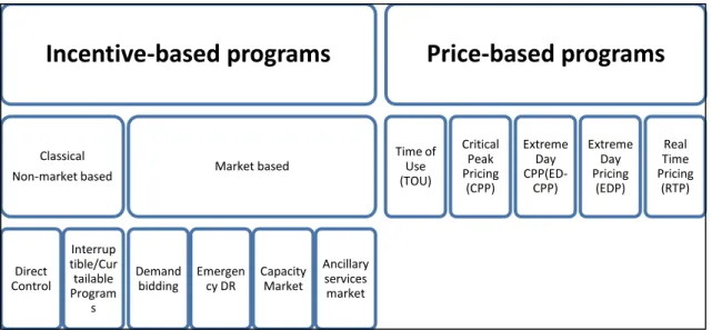
(14) 3. peak and off-peak rates. For example, a ToU of two-level of prices may charge a peak rate between 5 PM and 9 PM and an off-peak rate between 10 PM and 4 PM. Periods are established based on season, day of week, and time of day reflecting its true cost under those conditions. ToU rates incent customers to shift consumption from peak to off-peak periods to relieve the power system during higher demand scenarios.. Critical Peak Pricing (CPP) allows utilities to increase prices substantially during critical events, when the system is at its limit and action is required. Critical events are periods where the system operator anticipates that the power system could be reaching its maximum capacity. Generally, critical events last between 2 up to 24 hours in which wholesale prices would be extremely high. In return, customers receive discounts during non-critical periods. Typically, CPP is combined with ToU rates to account for both regular/periodic demand changes and extreme events.. Finally, RTP vary continuously (hour by hour) to reflect closely system conditions and wholesale prices (Moghaddam, Abdollahi, & Rashidinejad, 2011), providing a more efficient market clearing condition. RTP also incorporates implicitly the effects of weather, maintenance, time of day, and other factors affecting the supply and demand balance. RTP is the most dynamic rate as it changes hour to hour and day to day, but it is somewhat unpredictable for households, whose attention is not fully into electricity markets. In practice, since their demand is not following closely their preferences, price risk is all passed on to customers, who sometimes end up paying more (compared with a less dynamic but more predictable tariff).. Figure 1 shows different demand response programs classified under incentive-based and price-based programs (Dupont et al., 2011)..

(15) 4. Incentive-based programs. Classical. Direct Control. Time of Use (TOU). Market based. Non-market based. Interrup tible/Cur tailable Program s. Demand bidding. Emergen cy DR. Capacity Market. Price-based programs. Critical Peak Pricing (CPP). Extreme Day CPP(EDCPP). Extreme Day Pricing (EDP). Real Time Pricing (RTP). Ancillary services market. Figure 1: Types of demand response programs (adapted from Dupont et al (2011)) In well-organized electricity markets, dynamic electricity rates can reduce the cost of the system and these benefits can be passed on to customers through reductions in the price of the energy (Pollock & Shumilkina, 2010) and lower capacity costs (or capacity payments). One of the main goals of demand response programs is to reduce peak demand, as it determines the level of infrastructure (capacity) needed for electricity generation and transmission. A decrease of peak demand results in immediate savings for society as investments on infrastructure are delayed (less capacity is needed). A decrease of 5% of peak demand in the U.S., means a savings of U.S. 3 billion dollars per year (Faruqui, Hledik, Newell, & Pfeifenberger, 2007), (The Brattle Group, 2007). Energy price is also reduced as less efficient peaking are dispatched less frequently with dynamic electricity rates.. Most of these dynamic rates, ToU, CPP, and RTP require new investments in metering and some level of training cost for customers. In 2007, interval meters and smart meters used to enable these rates had an investment cost ranging from US$100 to US$200 (Faruqui et al., 2007) per meter. Nowadays, smart meters are the most common way to enable consumers to have tariff choices. They are slowly replacing interval meters that have. been. used. historically to. periodic/programmable rate.. enable. only ToU,. as. this. is. the. only.

(16) 5. During the last four decades several articles have studied dynamic electricity rates. They are reviewed in detail by Aigner, Caves, Parks, between others authors. (Aigner & Leamer, 1984; Aigner, 1984; D. Caves, Christensen, & Schoech, 1984; W. Caves, Christensen, & Herriges, 1984; Parks & Weitzel, 1984). While we don’t intend to review this large literature body, we do present some of the more recent work related to our model and analysis.. Several papers anticipated the benefits of dynamic pricing. More recent Bornstein and Holland (2005) analyzed the impact of RTP considering different proportions of consumers under this rate. They show that increasing the share of customers under RTP improves significantly market efficiency. To estimate the supply curve they assumed three levels of generation costs: a based load technology, a mid-merit technology, and a peaker technology. They simulated this for three levels of elasticities: -0.1, -0.3, and 0.4 and three levels of customers proportions under RTP: 33%, 66% and 100% of customers. With a third of customers on RTP they estimated a reduction on peaking capacity requirements of 44%. Kopsakangas and Svento (2012) analyzed the potential effects of RTP in the Nordic electricity market. As Borenstein and Holland (2005), they show that under RTP, capacity investments considerably decrease and total energy consumption increase with the demand elasticity if there is no emission trade. They estimated the supply curve using costs of different generation technologies including hydro power, nuclear power, conventional thermal power, and peak power technologies. They assumed an iso-elastic demand curve to perform their analysis.. Spees and Lave (2007) estimated the impacts of a ToU of two price levels and RTP in the PJM interconnection. They argued that flat rate is inefficient rate because it requires more capital in equipment than dynamic rates and is inequitable because customers with high coincident peak demand are being subsidized by all other customers.. They. estimated econometrically the supply curve and assumed an iso-elastic curve for the.

(17) 6. demand. They modeled using elasticities from 0 to -0.4 and their results show 10.4% of reduction in peak demand using an elasticity of -0.1 under RTP, while with the same elasticity but under a ToU rate of two price levels their results show 1.12% of peak demand reduction.. This paper develops an empirical economic model where the electricity supply curve is estimated econometrically and the electricity demand is calibrated hourly and assumed to be iso-elastic, allowing an exact match with wholesale real market data. The model is used to evaluate the effects in peak demand, energy consumption, and in the average cost of producing electricity with increasingly flexible price systems. We start from simple ToU rates, adding more price levels up to 24 within a day, aiming to assess the maximum theoretical benefit that can be obtained from periodic (and more predictable) rates. This is compared against RTP, the most flexible available tariff, assessing theoretically how much are the additional theoretical benefits from event-driven rates. A discussion of price periodic changes versus real-time event-driven changes is provided, as going beyond people (periodic) expectations may require more technology and may have limitations to “activate” customers. We also present a methodology to develop efficient ToU rates for comparing with CPP and RTP. The rest of this paper is divided as follows. Section II describes the PJM electricity market and the origin of the data. Section III presents and describes the proposed model. Section IV details the dynamic rates used as input in the model. Section V discusses the mains results. Finally, section VI presents the main findings and recommends future work to be done..

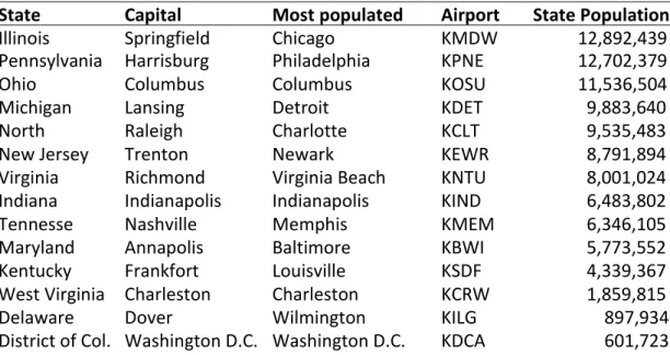
(18) 7. II. PENNSYLVANIA-NEW JERSEYMARKET AND DESCRIPTION OF DATA. MARYLAND. ELECTRICITY. In this paper we used public data on prices and capacity demand available on the Pennsylvania-New Jersey-Maryland (PJM) interconnection web site (PJM, 2010a). PJM interconnection serves more than 60 million people in a service area over 630,000 km2 including the states of Illinois, Pennsylvania, Ohio, Michigan, North Carolina, New Jersey, Virginia, Indiana, Tennesse, Maryland, Kentucky, West Virginia, Delaware, and the District of Columbia. In the case of temperature information we used public hourly data available in the Wunderground web site (Weather Underground, 2011); the hourly temperature is registered in meteorological stations of the airports in the most populated city of each state served by PJM. For every hour it is computed a population-weightedaverage of temperature data. Table 1 shows airport codes (used to retrieve temperature data from the Wunderground web site) and total population of each State (used for averaging the temperature data) according to 2010 US Census (US Census Bureau, 2011).. Table 1: S Airport codes used to retrieve temperature data from Wunderground website(Weather Underground, 2011) and total population by State according to the US 2010 Census (US Census Bureau, 2011) used for weighting temperature data State Illinois Pennsylvania Ohio Michigan North New Jersey Carolina Virginia Indiana Tennesse Maryland Kentucky West Virginia Delaware District of Col.. Capital Springfield Harrisburg Columbus Lansing Raleigh Trenton Richmond Indianapolis Nashville Annapolis Frankfort Charleston Dover Washington D.C.. Most populated Chicago city Philadelphia Columbus Detroit Charlotte Newark Virginia Beach Indianapolis Memphis Baltimore Louisville Charleston Wilmington Washington D.C.. Airport KMDW CODE KPNE KOSU KDET KCLT KEWR KNTU KIND KMEM KBWI KSDF KCRW KILG KDCA. State Population 12,892,439 12,702,379 11,536,504 9,883,640 9,535,483 8,791,894 8,001,024 6,483,802 6,346,105 5,773,552 4,339,367 1,859,815 897,934 601,723.

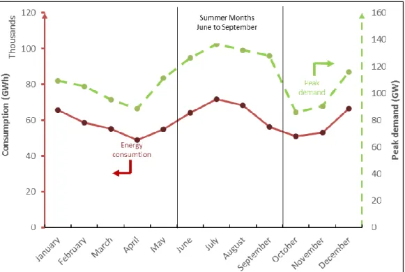
(19) 8. PJM demand description Within a year electricity power demand have seasonal, daily and hourly patterns. Capacity demand and energy consumption is especially high in summer months (June to September), particularly during days where the temperature exceeds 30°C. The annual peak power demand of 2010 reached 137 GW in July 06 (Tuesday at 5 pm). During warm months, the capacity demand and energy consumption decrease, but are back up again in the coldest months (December to March). The high consumption in the hottest and coldest months is explained essentially by the use of air conditioning systems which are extremely energy-intensive equipment. Figure 2 shows the actual monthly energy consumption and peak power demand for the PJM interconnection in 2010.. Figure 2: Energy consumption (GWh) and Peak power demand (GW) in PJM at 2010. In summer months (June to September) consumption and monthly peak demand increased respect to the rest of the year..

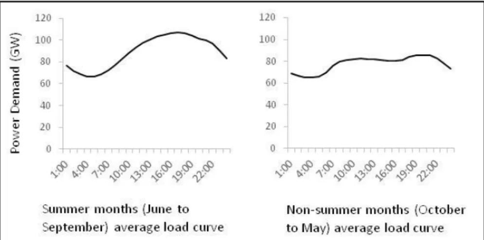
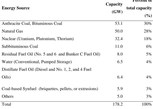
(20) 9. The hourly pattern of power demand is different depending on the season. The summer load profile reaches higher peaks at the afternoon (5 to 7 pm), while the load curve of the rest of the rest of the year has two pronounced peak, one at morning (9 to 11 am) and one at night (8 to 9 pm). Figure 3 shows the average load curve of summer months (June to September) and the rest of the year (October to May) of PJM 2010. The load factor (average load / maximum load) for the summer load curve was 83%, while for the rest of the year was 91%. This shows that in summer months, the infrastructure is not so well used as in the other months of the year and that in PJM the infrastructure level is determined by the summer demand.. Figure 3: Average daily load curve in summer months (June to September) and the rest of the year (October to May) are very different.. PJM supply description The fuel mix used to generate electricity in the PJM interconnection in 2010 was 36% of coal, 28% of natural gas, 18% of nuclear, and 18% of other fuels as is show in Table 2. This causes a very stable supply because the volatility of these energy sources is low. On the contrary, the supply curve of a power system based in hydro generation would suffer of shifts in time caused by the volatility of the hydro resource and the use of dams serving as electricity storage..

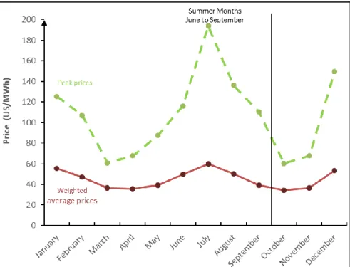
(21) 10. Table 2: Generation mix for PJM interconnection in 2010 according to the “2010 PJM Load, Capacity and Transmission Report” (PJM, 2010b). Capacity. Energy Source. (GW). Percent of total capacity (%). Anthracite Coal, Bituminous Coal. 53.1. 30%. Natural Gas. 50.0. 28%. Nuclear (Uranium, Plutonium, Thorium). 32.4. 18%. Subbituminous Coal. 11.0. 6%. Residual Fuel Oil (No. 5 and 6 and Bunker C Fuel Oil). 8.0. 5%. Water (Conventional, Pumped Storage). 6.5. 4%. Oils). 6.4. 4%. Coal-based Synfuel (briquettes, pellets, or extrusions). 5.9. 3%. Others. 5.0. 3%. 178.2. 100%. Distillate Fuel Oil (Diesel and No. 1, 2, and 4 Fuel. Total. A stable supply function causes that wholesale prices to have the same seasonality pattern as the capacity demand curve, although the price curve is more pronounced. As demand goes up, price also goes up but proportionately more; this is explained by a non-linear supply function. For example, energy consumption in July was 46% higher than in April (and 71,808 and 48,949 GWh respectively), while the wholesale price was 79% higher in July. (65.56 and 36.71 US$/MWh). Figure 4 presents the energy-. weighted-average price and the peak price per month for PJM in 2010; this figure presents the same pattern as the capacity demand curve (see Figure 2), high prices during summer months (June to September), low prices during warm months, and high prices during cold months (December to March)..

(22) 11. Figure 4: Monthly average price and peak price for PJM at 2010. Prices shows the same seasonality behavior as the demand.

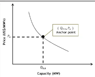
(23) 12. III.. ECONOMIC MODEL. We developed an economic model where the supply function is econometrically estimated from the actual data of prices and capacity of the PJM energy market. On the other side, the demand function is not econometrically estimated, but is calibrated hourly to capture not only the typical seasonal behavior of electricity demand, but also the exact actual value of capacity usage. Next, we present the details of the demand and supply function used in the model. Electricity demand function The main driver of the demand for electricity is not the price but the economic activity and the habits of consumers behind this demand. This is modeled though other factors like the hour of day, the day of the week, the month of the year, the temperature (highly correlated with the month of the year). The demand function should capture all these seasonality effects, to do so we calibrated a demand function for each of the 8,760 hours of the year. Using an hourly-based demand function we are able to capture, not only the hourly, daily and seasonal effects along the year (and with them implicitly the temperature effects) but also the exact actual value of capacity usage.. The demand curve used in the model is iso-elastic and is represented by the following expression term. , where the elasticity “e” is exogenous to the model. The. is determined using the “anchor point” of the curve that corresponds to the. actual capacity demand at hour system expression:. (different for every hour) and the average price for the. (same for every hour). Accordingly,. is defined by the following.

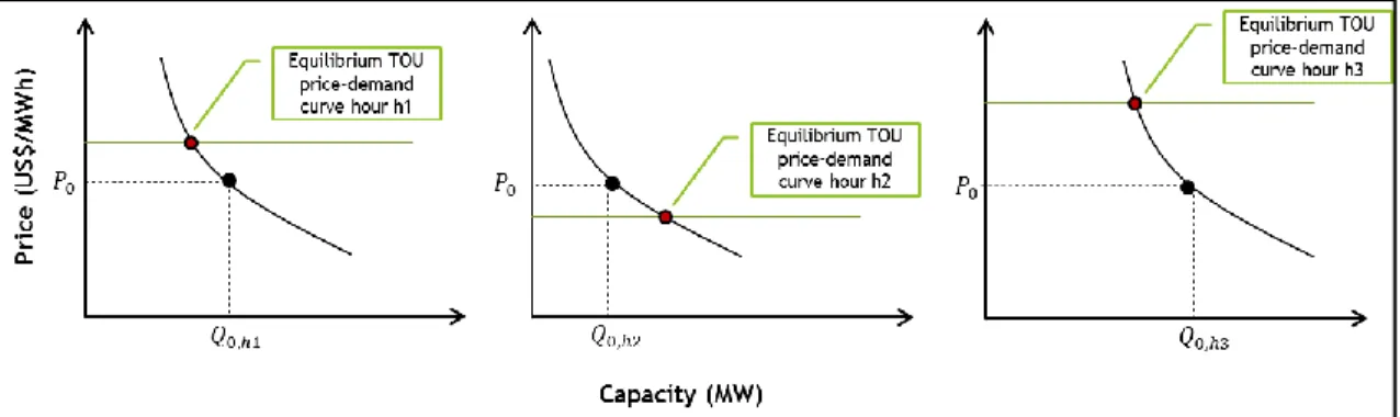
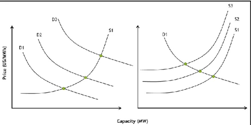
(24) 13. where. is the energy-weighted-average wholesale price for the year 2010; “e” is the. price elasticity (exogenous to the model); and. is the actual capacity demand at hour. “h”. Figure 5 shows an example of the demand curve used for hour. Figure 5: Example of demand curve used for hour “h”. The term. .. is different for. every hour of the year to capture hourly and seasonal effects of the demand. It should be noted that the demand is not econometrically estimated, thus the equation structure does not include demand shifters as time of day, month, temperature, etc. These factors are taken into account through the term. which varies by hour capturing. all periodic (seasonal, daily, etc.) and event-driven (exceptional hard to predict events) changes in demand. Electricity supply function The supply functions perceived by consumers differ depending on the type of rate they are facing; when consumers face a ToU or CPP rate they perceive a price-inelastic supply curve at every period because the price charged is independent of the demand. Thus, for the case of ToU or CPP evaluation, equilibrium between supply and demand occurs in the intersection between the demand curve and the price set for each period. Figure 6 shows three different periods, with different ToU rates, different demand.

(25) 14. functions, and their new equilibriums. In our evaluation, these new equilibrium points are computed for every hour of the year.. Figure 6: Three different ToU rates with different demand functions and new equilibriums points. Under RTP consumers face the actual supply as price varies according to the aggregate demand and the available supply. We estimated the actual supply curve econometrically as Spees & Lave (2008); however, we didn’t ignore the endogeneity between price and capacity demand. Methodologically is incorrect to estimate the supply curve directly from the equilibrium points, since it is not clear whether this estimates the actual supply curve, the demand curve or a mixture of both curves. Figure 7 shows two extreme cases, case (a) occurs when the supply does not shift in time, while the demand does. In this case equilibrium points map the supply curve. On the contrary, case (b) occurs when the supply curve shifts in time but the demand is fixed, so in this case equilibrium points map the demand curve. Actually, what happens in electricity markets is that both curves shift in time; the demand curve shifts in time mainly because of the hourly and seasonal consumption patterns related with the economic activity and the habits of consumers and the supply curve may shift in time because of changes in the availability of generators and resources. Although the supply curve may experience smalls shifts compared with demand, it is structurally incorrect to use equilibrium points to estimate it..

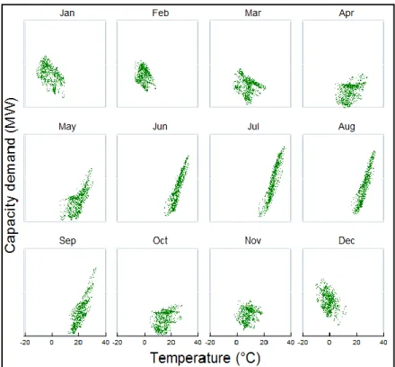
(26) 15. Figure 7: Case (a) Fixed supply with demand shifting in time (left) cause that equilibrium points map the supply curve, and - Case (b) fixed demand and supply shifting in time (right) cause that equilibrium points map the demand curve.. To estimate the supply curve without bias and correct the endogeneity problem it should be used instrumental variables that shift the demand curve and does not shift the supply curve. In this work we used as instrumental variables the time of day and the temperature per month. The time of day is included as fixed effect of the demand, while the temperature per month is included as continuous variable as is show in Eq. (2).. The temperature shifts the demand curve because climate control systems raise capacity demand, particularly in periods of extreme temperatures (Lee & Chiu, 2011; Pardo, Meneu, & Valor, 2002). As is show in Figure 8, in PJM there is a strong relationship between the energy demand and temperature. There is a positive correlation in the hottest months (June to September) and a negative correlation in the coldest months (December to March)..

(27) 16. Figure 8: Capacity demand (MW) vs. temperature (°C) showing the positive correlation between temperature and demand in summer month (June to September) and the negative correlation in other month (December to March). To incorporate the instrumental variables in the estimation of the supply curve, it is performed a Two Stage Least Square (TSLS or 2SLS) regression. For the first stage regression, we used a second order polynomial function which incorporates hourly dummy variables in the intercept and monthly dummy variables in the first order terms. Thereby, we considered in the first stage of the regression the fixed effects of the time of day and the monthly effects of temperature. Eq (2) shows the structural equation used for this regression:. Where. corresponds to dummy variables to separate the effect of each hour. corresponds to dummy variables to separate the effect of each month. , and. , is.

(28) 17. the temperature (plus an offset to avoid negative numbers). Almost all the estimated parameters are statistically significant at 5% level as show in Table 3.. Table 3: Regression parameters of the first stage regression, almost all parameter are statically significant at a 5% level except of the hourly fixed effect at 6 am and the monthly February temperature Source. SS. df. MS. Model Residual. 1.9463e+12 2.5489e+11. 46 8711. 4.2310e+10 29260719.8. Total. 2.2012e+12. 8757. 251361371. Std. Err.. t. Number of obs F( 46, 8711) Prob > F R-squared Adj R-squared Root MSE P>|t|. = 8758 = 1445.98 = 0.0000 = 0.8842 = 0.8836 = 5409.3. demand. Coef.. [95% Conf. Interval]. hour 2 3 4 5 6 7 8 9 10 11 12 13 14 15 16 17 18 19 20 21 22 23 24. -2597.991 -3953.084 -4372.348 -3449.352 -176.1441 5472.292 9712.912 11432.39 12334.92 13052.7 13215.63 13112.51 12919.3 12626.02 12442.68 13214.33 14840.27 15310.05 15202.05 15535.78 14115.53 9718.152 4340.668. 400.5067 401.0369 401.1071 401.4969 401.9446 402.42 402.1676 401.0049 400.6058 401.9207 404.4993 407.4597 410.2827 412.3713 413.4865 413.2019 411.6214 409.2833 406.4404 403.7266 401.8981 401.0051 400.8481. -6.49 -9.86 -10.90 -8.59 -0.44 13.60 24.15 28.51 30.79 32.48 32.67 32.18 31.49 30.62 30.09 31.98 36.05 37.41 37.40 38.48 35.12 24.23 10.83. 0.000 0.000 0.000 0.000 0.661 0.000 0.000 0.000 0.000 0.000 0.000 0.000 0.000 0.000 0.000 0.000 0.000 0.000 0.000 0.000 0.000 0.000 0.000. -3383.078 -4739.211 -5158.613 -4236.381 -964.0504 4683.453 8924.569 10646.32 11549.63 12264.84 12422.71 12313.8 12115.05 11817.68 11632.15 12404.35 14033.39 14507.76 14405.33 14744.38 13327.72 8932.088 3554.911. -1812.903 -3166.957 -3586.084 -2662.323 611.7623 6261.13 10501.26 12218.45 13120.2 13840.56 14008.54 13911.23 13723.55 13434.37 13253.22 14024.3 15647.14 16112.34 15998.77 16327.18 14903.35 10504.22 5126.425. month 2 3 4 5 6 7 8 9 10 11 12. 2772.873 -11641.97 -50214.3 -88596.9 -161298.9 -187766.8 -179876.1 -127975.7 -49174.61 -28891.05 6172.372. 1640.92 1453.982 1673.851 1826.704 2733.366 2740.624 2792.677 2215.305 1721.187 1666.553 1298.085. 1.69 -8.01 -30.00 -48.50 -59.01 -68.51 -64.41 -57.77 -28.57 -17.34 4.75. 0.091 0.000 0.000 0.000 0.000 0.000 0.000 0.000 0.000 0.000 0.000. -443.7175 -14492.12 -53495.44 -92177.67 -166656.9 -193139 -185350.4 -132318.2 -52548.54 -32157.89 3627.818. 5989.463 -8791.826 -46933.16 -85016.13 -155940.8 -182394.5 -174401.8 -123633.2 -45800.67 -25624.21 8716.925. month#c.temp 1 2 3 4 5 6 7 8 9 10 11 12. -1279.69 -1430.257 -940.1727 164.7418 1268.289 3087.637 3687.348 3492.861 2252.441 150.2017 -356.143 -1538.596. 40.54367 73.47612 43.49467 42.54104 42.13137 59.0401 56.7351 59.13433 50.23355 44.28469 52.41083 53.70136. -31.56 -19.47 -21.62 3.87 30.10 52.30 64.99 59.07 44.84 3.39 -6.80 -28.65. 0.000 0.000 0.000 0.000 0.000 0.000 0.000 0.000 0.000 0.001 0.000 0.000. -1359.165 -1574.288 -1025.433 81.35133 1185.702 2971.905 3576.134 3376.944 2153.972 63.39327 -458.8807 -1643.863. -1200.215 -1286.226 -854.9129 248.1323 1350.877 3203.37 3798.562 3608.778 2350.911 237.0102 -253.4054 -1433.329. _cons. 103949.2. 834.0781. 124.63. 0.000. 102314.2. 105584.2.

(29) 18. For the second stage regression (price over the estimated capacity. ), it is used a. squared polynomial function to capture the non-linearity of the supply curve between price and capacity. To implicitly take into account the changes in the supply structure, we incorporated monthly dummies in the intercept and in the first order term as is shown in Eq (3).. Where is a dummy variable for each day, is the estimated demand (first stage regression), and is the wholesale price. Almost all parameters estimated for this regression were statistically significant at a 5% level as is show in Table 4. Only the monthly fixed effect of December resulted statistically non-significant. Table 4: Regression parameters of the second stage regression. Only the monthly fixed effect of June and December resulted statistically non-significant. Source. SS. df. MS. Model Residual. 2390983.17 734332.13. 24 8733. 99624.2989 84.0870411. Total. 3125315.3. 8757. 356.893377. Coef.. month 2 3 4 5 6 7 8 9 10 11 12. 36.01633 25.54403 9.718506 24.94799 57.85382 53.10018 64.73585 40.31156 18.42942 28.59285 -3.766107. 6.106738 5.510764 5.177303 4.508006 4.11339 4.093455 4.071424 4.214281 5.17259 5.538406 5.320134. 5.90 4.64 1.88 5.53 14.06 12.97 15.90 9.57 3.56 5.16 -0.71. 0.000 0.000 0.061 0.000 0.000 0.000 0.000 0.000 0.000 0.000 0.479. 24.04568 14.74163 -.4302276 16.11124 49.79061 45.07604 56.7549 32.05058 8.289925 17.73627 -14.19482. 47.98697 36.34642 19.86724 33.78475 65.91704 61.12431 72.7168 48.57255 28.56892 39.44943 6.662609. -.0019719 -.0024506 -.0022682 -.0019692 -.0022343 -.0027492 -.0027154 -.0028667 -.0025152 -.0021249 -.0022991 -.0019766. .0001054 .000111 .0000976 .0000866 .0000857 .0000995 .0001069 .0001029 .0000897 .000087 .0000956 .000107. -18.70 -22.08 -23.25 -22.74 -26.07 -27.62 -25.41 -27.85 -28.05 -24.42 -24.05 -18.48. 0.000 0.000 0.000 0.000 0.000 0.000 0.000 0.000 0.000 0.000 0.000 0.000. -.0021786 -.0026682 -.0024595 -.0021389 -.0024023 -.0029443 -.0029249 -.0030685 -.002691 -.0022954 -.0024865 -.0021863. -.0017652 -.0022331 -.002077 -.0017994 -.0020663 -.0025541 -.0025059 -.002665 -.0023394 -.0019544 -.0021118 -.0017669. 2.19e-08 57.61456. 5.59e-10 5.541391. 39.13 10.40. 0.000 0.000. 2.08e-08 46.75212. 2.30e-08 68.47699. dem_pre2 _cons. t. P>|t|. = 8758 = 1184.78 = 0.0000 = 0.7650 = 0.7644 = 9.1699. lmp_da_rt. month# c.dem_pre 1 2 3 4 5 6 7 8 9 10 11 12. Std. Err.. Number of obs F( 24, 8733) Prob > F R-squared Adj R-squared Root MSE. [95% Conf. Interval].

(30) 19. IV. RATES APPLIED TO THE MODEL The inputs to the model are different ToU rates, ToU-CPP rate, and RTP rate; all the results are compared with the base case (flat rate pricing). We tested a ToU of two price levels combined with a CPP rate considering only five critical events in the year with a duration of three hours each and with a maximum of one event per calendar day. Finally, we tested a RTP scheme where consumers face an hourly rate that varies every day. This selection of rates allow us (at the limit) assessing the effects of periodic rates, separately from the effect of event-driven real-time rates. We are able to quantify what we call the “response premium” that can be theoretically obtained when customers respond perfectly to real-time rates instead of constantly changing periodic rates. TOU: number of prices levels We defined ToU rates with different degrees of dynamism; this is ToU rates with two, three, five, and 24 levels of prices within a day. A ToU rate with five levels of price in a day is a much more dynamic rate than a ToU of two levels. However, a ToU rate is not only defined by the number of price levels in a day, but also by the moment of the day (time blocks) in which each price is applied and by the magnitude of the price. The ToU with 24 price levels has not been actually used before both in companies or in the literature, but it is the most dynamic rate that can be applied with some interval meters, as well as the maximum resolution market data available for PJM. ToU rates are based on periodic supply/demand changes and ToU-24 is the most dynamic periodic rate that can be applied.. TOU: hours of the day where each price level is applied To identify the moment of the day where each level of price is charged, we used the average-price-duration curve. This is done for summer months (June to September) and for the other months of the year (October to May) independently. Figure 9 shows the case ToU rate of five price levels for summer months, where the duration curve was divided into five to separate the hours. Using this methodology we identified the.

(31) 20. periods of the ToU rate with two, three, and five price levels, differencing summer months with the rest of the year. For the ToU rate with 24 price levels separation is trivial because each hour of the day represent one different period.. Figure 9: Average duration curve for summer month (June to September) segmented to identify the hours of each time block in a day.. Note that using this methodology the resulting ToU rate can present time blocks of only one hour. For example, in the case presented in Figure 9 the hour 19 (7 pm) is isolated because before is the time block that includes hours 15, 16, 17, and 18 and after is the time block that includes hours 20, 21, and 22 as is shown in the ToU of 5 levels presented in Figure 10 . Although this may be unpractical, we used this methodology to be able to compare our results between the different ToU rates and with RTP, thus modeling increasing levels of price flexibility..

(32) 21. Figure 10: Example of the blocks time in a day with ToU of 2,3 and 5 price levels. TOU: magnitude of each price level To determine the price level at each ToU period it is applied the "revenue neutral" principle; this is, the ToU price of a defined ToU period should be the same in average (during the year) to the price in the wholesale energy market in the same period. This is computed in an iteratively process because ToU price affects the wholesale price through a change in the demand as shows Figure 11. The change in capacity demand caused by the ToU rate is computed using the demand curve and the change in the wholesale prices is computed using the supply curve. New ToU prices are determined averaging the wholesale price in a period, then is computed the change in the demand, and then the change in the wholesale price. This iteratively process is done until convergence. Demand function. ToU price in period "t". Supply function. Change in capacity demand. Change in wholesale prices. Energy-weighted-average wholesale price in period “t”. Figure 11: ToU prices affect wholesale prices through a change in the demand.

(33) 22. It should be noted that using this methodology the ToU prices at every period depend in the model and the price elasticity. Therefore, for every elasticity the price at each period changes. For example, for the ToU rate of two price levels the price is different depending if the price elasticity is -0.1 or -0.4 as is shows in Figure 12. The more elastic is the demand, the greater is the response to price changes, so it is required less. 65 45. 55. e= -0.1. e= -0.4. 35. Price (US$/MWh). 75. difference between the prices set at each period to get the same results.. 1. 3. 5. 7. 9. 11. 13 Hour. 15. 17. 19. 21. 23. Figure 12:ToU of two price levels with different prices for each period. ToU rate vary according to the price elasticity "e".. TOU2 – CPP rate The model also received as input a ToU with two price levels combined with a CPP rate. A CPP rate allows increasing price to customers during critical events; critical events are periods where it is anticipated that the power system could be reaching its maximum demand level. Critical events vary in number and time duration in the year; the duration of the events could last between two hours up to one day. These parameters, number of events and duration of the events, are generally predetermined by the utility. For example, Pacific Gas and Electric Company (PG&E) define 6 hours for each event; in the first three hours it charges three times the ToU off peak rate and in the.

(34) 23. last three hours it charges five times this value (Pollock & Shumilkina, 2010). Southern California Edison applies 9 to 15 events in a year of 4 hours each (Edison, 2012). During 2010, in PJM the five first critical events (extremely high wholesale prices) occurred in July and then the maximum wholesale peaks occurred alternately in December and July. Since in PJM the infrastructure level is determined by the highest peaks in the summer period, in this paper we tested a CPP rate considering the first five events in a year with three hours duration.. During critical events the price can be raised between three to ten times over the flat rate. The CPP rate could be approximated to high spot market prices, which may exceed up to ten times the average price of electricity. During 2010, the highest wholesale price in PJM reached 194 US$/MWh (July 07 at 5 pm), this is almost four times higher than the average wholesale price of 49.9US$/MWh.. Consequently, we used 200. US$/MWh as the critical event price. Figure 13 shows the first seven critical events in time-windows of three hours for PJM during 2010 and its actual wholesale prices. In summary, for the ToU2-CPP rate almost all days is charged a ToU of 2 price levels except in the following days between 4 pm and 6 pm, in which is charged a special a rate of 200 US$/MWh: July 07, July 06, July 23, July 16, and July 24..

(35) 24. Figure 13: Critical events in PJM 2010 interconnection. The first 5 critical events occurred in July at 5 pm. RTP rate RTP rate does not require any design as the price and quantity for each hour is simply determined by the equilibrium point between the demand and the actual supply curve. Using the estimated demand and supply curve we computed for each hour a new equilibrium point. This yields in a different price for every hour for each day. RTP represents the highest degree of dynamism and therefore its effects on the load curve and prices represent an extreme (but often unachievable) case..

(36) 25. IV.. NUMERICAL RESULTS. We have modeled different dynamic rates assuming that these rates are mandatory for the 100% of the demand, and have evaluated the impacts in peak demand, overall energy demand, and average cost of electricity production. As was expected, effects under ToU rates are fractions of effects under RTP. However, with a simple ToU of two price levels combined with a CPP rate of 5 events in a year, the peak demand reduction is notable increased. Finally, the effects under RTP are stand out above the rest because with a very small elasticity it reaches high peak demand reduction. Table 5 to show peak load (GW), total energy (TWh), total expense (US$ Billions), and average price (US$/MWh) for each rate and elasticity, while Figure 14 to Figure 16 show graphically peak reduction (%), consumption increase (%), and consumer expense saved(%) for each rate and elasticity.. Table 5: Peak load, energy consumption, total expense, and average price for ToU 2, ToU 3, ToU 5, ToU 24, ToU 2 - CPP, and RTP for elasticities from -0.1 to -0.4. Effects of ToU 2 (two price levels) Elasticity 0 -0.1 -0.2 -0.3 -0.4. Peak Load (GW) 136.68 132.67 130.28 128.69 128.27. Total Energy (TWh) 713.88 716.02 718.00 719.64 720.97. Expense (US$ Billions) 34.23 33.81 33.74 33.78 33.85. Average Price ($/MWh) 47.95 47.22 47.00 46.94 46.95. Effects of ToU 5 (four price levels) Elasticity 0 -0.1 -0.2 -0.3 -0.4. Peak Load (GW) 136.68 131.73 128.85 126.94 125.76. Total Energy (TWh) 713.88 716.75 719.56 721.95 723.94. Expense (US$ Billions) 34.23 33.69 33.59 33.62 33.71. Average Price ($/MWh) 47.95 47.01 46.68 46.57 46.56. Effects of ToU 3 (three price levels) Elasticity 0 -0.1 -0.2 -0.3 -0.4. Peak Load (GW) 136.68 131.90 130.22 129.14 128.35. Total Energy (TWh) 713.88 716.47 718.94 721.01 722.70. Expense (US$ Billions) 34.23 33.74 33.65 33.68 33.76. Average Price ($/MWh) 47.95 47.09 46.80 46.72 46.72. Effects of ToU 24 (24 price levels) Elasticity 0 -0.1 -0.2 -0.3 -0.4. Peak Load (GW) 136.68 131.52 128.52 126.54 125.12. Total Energy (TWh) 713.88 716.92 719.95 722.57 724.75. Expense (US$ Billions) 34.23 33.66 33.55 33.58 33.67. Average Price ($/MWh) 47.95 46.96 46.60 46.47 46.45.

(37) 26. Effects of RTP Elasticity 0 -0.1 -0.2 -0.3 -0.4. Peak Load (GW) 136.68 126.21 120.79 118.66 117.20. Effects of ToU 2 - CPP Total Energy (TWh) 713.88 719.56 725.02 729.75 733.74. Expense (US$ Billions) 34.23 33.21 33.01 33.07 33.22. Average Price ($/MWh) 47.95 46.15 45.53 45.32 45.28. Elasticity 0 -0.1 -0.2 -0.3 -0.4. Peak Load (GW) 136.68 130.68 128.42 127.34 128.27. Total Energy (TWh) 713.88 716.07 718.09 719.75 721.10. Expense (US$ Billions) 34.23 33.80 33.73 33.77 33.84. Average Price ($/MWh) 47.95 47.20 46.97 46.92 46.93. Peak reduction ToU rates schemes with two or three price levels succeed in reducing a large portion of the annual peak demand. Considering an elasticity of -0.1, peak demand is reduced a 2.9% with a 2-level ToU up to 3.8% with a 24-level ToU respect to the flat rate. With the same elasticity, the ToU2-CPP rate reached a peak demand reduction of 4.4%. On the other side, with RTP the peak demand is reduced 7.7%. These results show that increasing the extent of dynamism of the rates does not translate into big benefits of peak demand reduction. A simple ToU of two price levels combined with a CPP rate of only five events in a year achieved a peak demand reduction of more than a half of the reduction caused by the implementation of RTP, where rates are changing each hour of the year..

(38) 27. Responding to Periodic (more predictable) demand Changes. Responding to Real-time (less predictable) demand Changes. “Response premium” due to Real-time data. Figure 14: Peak reduction (%) per type of rate and elasticity respect to flat rate. Energy Consumption The higher is the price elasticity of demand and the extent of dynamism of the rate, the higher is the aggregate energy consumption. Consumers reduce their energy consumption when prices are high, but also raise their consumption when prices are low. The overall result of these two effects is an increase in energy consumption (by up to 2.8% with RTP with an elasticity of -0.4) compared to the base case (flat rate). In terms of a pure economics point of view, an increase in consumption caused benefits for society (if the cost does not increase) because means more consumer surplus. In terms of emissions reduction, the effects of dynamic rates depend in the fuel mix of the supply. Under RTP, emissions reduction occur in regions with more oil-fired capacity than hydroelectric (Holland & Mansur, 2004), so environmental benefits of dynamic rates depend in the region where they are to be applied. In the case of PJM, electricity generation is based on coal, natural gas and nuclear, as a result “demand response is seen as more green-friendly because reducing and/or shifting electricity use translates to reducing emissions”.

(39) 28. Responding to Periodic (more predictable) demand Changes. “Response premium” due to Real-time data. Responding to Real-time (less predictable) demand Changes. Figure 15: Consumption increase (%) per type of rate and elasticity respect to flat rate. Consumer expense With all dynamic rates the average consumer expense is reduced compared with the flat rate. However, savings does not always increase with elasticity as energy consumption. When consumers are very price-inelastic (elasticity >= -0.1) savings comes from peak demand reduction (consumers stop demanding when prices are high). On the other hand, when consumers show some response to change in prices (elasticity <= -0.2), the effect of overall increase in consumption become more important and affect savings. These results are consistent with those shown by Spees and Lave (2008).

(40) 29. Responding to Periodic (more predictable) demand Changes. “Response premium” due to Real-time data. Responding to Real-time (less predictable) demand Changes. Figure 16: Average consumer expense saved (%) per type of rate and elasticity. Dynamic rates are beneficial for society (compared with flat rates) as peak consumption is reduced and electricity infrastructure is better utilized. Lower prices under off-peak conditions leads to an increase in overall use of electricity, but consumers bills are reduced as energy prices (in average) are lower. While RTP is theoretically superior to ToU, a simple ToU with two price levels is able to capture nearly half of the benefits from RTP, paying fractions of the implementation costs. In addition, for residential users is very difficult to manage a very dynamic rate as they do not have the interest and the tools to be aware and continuously response to changing prices. Finally, there are limited studies evaluating of how dynamic-pricing impact on equity, being that a key concern on the developing world. Pilot programs have showed that low-income customers do not respond to change in prices, as high-income customers do. Therefore, implementing a dynamic rates could potentially harm poor people (increasing their electricity bill), instead of help them (Alexander, 2010)..

(41) 30. V.. CONCLUSIONS AND DISCUSSION. In this paper we have developed a model to evaluate the impact of different dynamic rates in energy demand and prices. We modeled the supply curve by estimating it from actual PJM price-capacity equilibrium points and we corrected endogeneity using hourly fixed effect and temperature as instrumental variables. In the case of demand, it is assumed an iso-elastic function and it adjusted using actual consumption of PJM for each hour of the year assuming elasticities from -0.1 to -0.4. The use of the actual consumption at each hour allows drawing more accurate conclusions regarding capacity utilization and benefits from peak reductions.. Three common qualitative effects emerged from the analysis of these dynamic rates: 1) Dynamic pricing encourages peak demand reduction leading to lower capital costs (lower infrastructure capacity is needed). However, price-based programs does not ensure 100% a specific reduction amount of peak demand, as traditional incentive based programs do (where utilities takes direct control of loads). 2) Dynamic pricing results in higher energy consumption during the year. From an economic point of view, this is positive because more consumption at lower cost means more welfare. However, from an emissions perspective, the benefit depends on the fuel mix of the supply, because emissions reductions occur in regions with more oil-fired capacity than hydroelectric (Holland & Mansur, 2004). 3) Dynamic pricing causes a reduction of average cost as result of an increase in electricity consumption at hours where the production cost is low and a decrease at hours where the production cost is high. This causes a lower average energy cost compared with flat rate.. This paper contributes to explain why utilities and policy makers rushed into real-time rates experiments. Neglecting real-life and implementation issues dynamic rates are conceptually highly beneficial (flexibility is always welfare enhancing). Most basic economic models (including ours) are able to capture the value of real-time data, but they are not able to capture real-life and implementation issues, communicating and.

(42) 31. activating consumer’s response.. Under these models CPP offers limited benefits. compared with RTP. Why getting consumer response only a few hours (with CPP), if you can get the response at every hour (with RTP)? Why expending a lot of money in a few hours (with CPP) if you can pay a just a bit more for peak hours (with RTP)?. CPP or TOU plus CPP based its success in benefits that are hard to consider in supply and demand models. While ToU realizes the benefits from periodic (and easy to get used to) price changes, CPP does it best in activating consumers when it is truly necessary. RTP seems too ambitious; aiming to get customers to optimal response always, at every hour of the year, while CPP recognize that customer response limitations and their willingness to respond only when price changes are high enough to make it worth the trouble. Traditional ToU rates have exploited the easy portion of peoples’ demand respond capability, as periodic demand changes with two or three rates are easily factored in at people’ routines without imposing significant cost in their lifestyles. Pushing these changes to 24 hourly price steps provide only marginal additional benefits and as it is hard to keep in mind 24 rate levels, they would be hard to factor in and the marginal benefits found (theoretically) in this paper would be more likely not realized.. People face adjustments costs, changing behavior is costly and getting the information to trigger these changes is also costly. Most (if not all) supply/demand economic models somewhat neglect factoring in the limitations activating customers response. Realizing the “response premium” due to real-time data beyond periodic rate changes is costly, requires a customer to be focused on the price of the system and requires devices to enable communication and maximize this response, such as cell phone messages, alarms, visual aids (e.g. energy orbs), etc. rewarded enough to pay for the trouble.. This also requires the customer to be.

(43) 32. This reward must be higher than the adjustment costs faced by the customer (plus the enabling technology costs if the customer has to pay it). While RTP hardly ever satisfy this relationship, CPP often does it, targeting the reward/penalty exactly at the moment when customer response is needed.. Despite of the positive economic results of dynamic rates, these are not enough to recommend its implementation in any country. It must be taken into account the direct costs of implementing dynamic pricing such as meters, communications, new billing systems, and other infrastructure costs, as well as training customers and utility staff. There are also indirect social costs such as loss of welfare of consumer for being forced to stay alert to changes in electricity prices or responding sub-optimally to price changes. Only people with high and/or special loads like, air conditioning system and pools, can ensure benefits by simply optimizing their consumption by programming their devices. Finally, economics benefits quantified in this work are aggregated (for the whole society) and we have not performed the analysis of the distribution of these benefits; if dynamic electricity rates benefits rich people and harms poor people, then new mechanisms should be studied to redress this situation. This is of growing concern in developing countries..

(44) 33. REFERENCES Aalami, H. a., Moghaddam, M. P., & Yousefi, G. R. (2010). Demand response modeling considering Interruptible/Curtailable loads and capacity market programs. Applied Energy, 87(1), 243–250. doi:10.1016/j.apenergy.2009.05.041 Aigner, J. (1984). The welfare econometrics of peak-load pricing for electricity. Journal of Econometrics, 26, 1–15. Aigner, J., & Leamer, E. (1984). Estimation of Time-of-Use Pricing Responses in the Absence of Experimental Data. J. of Econometrics, 26, 205–227. Retrieved from http://scholar.google.com/scholar?hl=en&btnG=Search&q=intitle:Estimation+of+time+ of+use+pricing+response+in+the+absence+of+experimental+data#7 Albadi, M. H., & El-Saadany, E. F. (2008). A summary of demand response in electricity markets. Electric Power Systems Research, 78(11), 1989–1996. doi:10.1016/j.epsr.2008.04.002 Alexander, B. R. (2010). Dynamic Pricing? Not So Fast! A Residential Consumer Perspective. The Electricity Journal, 23(6), 39–49. doi:10.1016/j.tej.2010.05.014 Borenstein, S., & Holland, S. (2005). On the efficiency of competitive electricity markets with time-invariant retail prices. The Rand Journal of Economics, 36(3), 469– 493. Bureau, U. S. C. (2011). US 2010 Census. Retrieved October 09, 2011, from http://www.census.gov/2010census/ Cappers, P., Goldman, C., & Kathan, D. (2010). Demand response in U.S. electricity markets: Empirical evidence. Energy, 35(4), 1526–1535. doi:10.1016/j.energy.2009.06.029 Caves, D., Christensen, L., & Schoech, P. (1984). A comparison of different methodologies in a case study of residential time-of-use electricity pricing: Cost– Benefit Analysis. Journal of Econometrics, 26, 17–34. Retrieved from http://www.sciencedirect.com/science/article/pii/0304407684900113 Caves, W., Christensen, L. R., & Herriges, J. A. (1984). Consistency of residential customer response in time of use electricity pricing. Journal of Econometrics, 26, 179– 203. Dupont, B., De Jonghe, C., Kessels, K., & Belmans, R. (2011). Short-term consumer benefits of dynamic pricing. 2011 8th International Conference on the European Energy Market (EEM), (May), 216–221. doi:10.1109/EEM.2011.5953011.

(45) 34. Edison, S. C. (2012). Critical Peak Pricing Rate Schedule. Retrieved May 05, 2012, from https://www.sce.com/NR/rdonlyres/672CFB73-002B-4CA5-8E86B8F481E41A48/0/0909_CPPFactSheet.pdf Faria, P., & Vale, Z. (2011). Demand response in electrical energy supply: An optimal real time pricing approach. Energy, 36(8), 5374–5384. doi:10.1016/j.energy.2011.06.049 Faruqui, A., Hledik, R., Newell, S., & Pfeifenberger, H. (2007). The Power of 5 Percent. The Electricity Journal, 20(8), 68–77. doi:10.1016/j.tej.2007.08.003 FERC. (2013). Reports on Demand Response & Advanced Metering. Retrieved December 01, 2013, from http://www.ferc.gov/industries/electric/indus-act/demandresponse/dem-res-adv-metering.asp Holland, S., & Mansur, E. T. (2004). Is Real-Time Pricing Green ? The Environmental Impacts of Electricity Demand Variance Mansur. Review of Economics Statistics, 90, 550–561. Kopsakangas Savolainen, M., & Svento, R. (2012). Real-Time Pricing in the Nordic Power markets. Energy Economics, 34(4), 1131–1142. doi:10.1016/j.eneco.2011.10.006 Lee, C.-C., & Chiu, Y.-B. (2011). Electricity demand elasticities and temperature: Evidence from panel smooth transition regression with instrumental variable approach. Energy Economics, 33(5), 896–902. doi:10.1016/j.eneco.2011.05.009 Moghaddam, M. P., Abdollahi, a., & Rashidinejad, M. (2011). Flexible demand response programs modeling in competitive electricity markets. Applied Energy, 88(9), 3257–3269. doi:10.1016/j.apenergy.2011.02.039 Mojtahedzadeh, S., Tavakoli, M. A., & Milani, A. R. (2011). Review of dynamic pricing programs and evaluating their effect on demand response. Technical and Physical Problems of Engineering, 3(3), 100–105. Pardo, A., Meneu, V., & Valor, E. (2002). Temperature and seasonality influences on Spanish electricity load. Energy Economics, 24(1), 55–70. doi:10.1016/S01409883(01)00082-2 Parks, R., & Weitzel, D. (1984). Measuring the consumer welfare effects of timedifferentiated electricity prices. Journal of Econometrics, 26, 35–64. Retrieved from http://www.sciencedirect.com/science/article/pii/0304407684900125 PJM. (2010a). PJM Energy Market. Retrieved December 01, 2013, from http://www.pjm.com/markets-and-operations/energy.aspx.

(46) 35. PJM. (2010b). PJM Energy Information Agency (EIA) Reports. Retrieved from http://www.pjm.com/documents/reports/eia-reports.aspx Pollock, A., & Shumilkina, E. (2010). How to Induce Customers to Consume Energy Efficiently : Rate Design Options and Methods. Retrieved from http://www.nrri.org/pubs/electricity/NRRI_inducing_energy_efficiency_jan10-03.pdf Spees, K., & Lave, L. (2008). Impacts of Responsive Load in PJM: Load Shifting and Real Time Pricing. The Energy Journal, 29(2). doi:10.5547/ISSN0195-6574-EJ-Vol29No2-6 The Brattle Group. (2007). Quantifying Demand Response Benefits In PJM. Wang, J., Bloyd, C. N., Hu, Z., & Tan, Z. (2010). Demand response in China. Energy, 35(4), 1592–1597. doi:10.1016/j.energy.2009.06.020 Weather Underground, I. (2011). Wunderground Weather. Retrieved October 08, 2011, from http://www.wunderground.com/.

(47)