A kernel regression procedure in the 3D shape space with an application to online sales of children's wear

Texto completo

(1)A kernel regression procedure in the 3D shape space with an application to online sales of children’s wear Gregorio Quintana-Ortia,c , Amelia Simób,c a. Department of Computer Science and Engineering. b Department of Mathematics-IMAC. c Universitat Jaume I. Avda. del Riu Sec s/n. 12071-Castellón, Spain.. Abstract Shape regression is of key importance in many scientific fields. In this paper, we focus on the case where the shape of an object is represented by a configuration matrix of landmarks. It is well known that this shape space has a finite-dimensional Riemannian manifold structure (non-Euclidean) which makes it difficult to work with. Papers about regression on this space are scarce in the literature. The majority of them are restricted to the case of a single explanatory variable, usually time or age, and many of them work in the approximated tangent space. In this paper we adapt the general method for kernel regression analysis in manifold-valued data proposed by Davis et al (2007) to the three-dimensional case of Kendall’s shape space and generalize it to multiple explanatory variables. We also propose bootstrap confidence intervals for prediction. A simulation study is carried out to check the goodness of the procedure, and finally it is applied to a 3D database obtained from an anthropometric survey of the Spanish child population with a potential application to online sales of children’s wear. Keywords: Shape space, Statistical shape analysis, Kernel regression, Fréchet mean, Children’s wear 1. Introduction Many problems in medical imaging analysis and computer vision involve predicting the shape of an object as a function of a set of covariates (age, Email addresses: gquintan@uji.es (Gregorio Quintana-Orti), simo@uji.es (Amelia Simó) Preprint submitted to Computational Statistics and Data Analysis. July 12, 2016.

(2) dose, etc.). A significant amount of research and activity has been carried out in recent decades in the general area of shape analysis. By shape analysis, we mean a set of tools for comparing, matching, deforming, and modeling shapes. Three major approaches can be identified in shape analysis based on how the object is treated in mathematical terms (Stoyan and Stoyan, 1995): Objects can be treated as subsets of Rm , they can be described as sequences of points that are given by certain geometrical or anatomical properties (landmarks), or they can be defined using functions representing their contours. The majority of research has been restricted to landmark-based analysis, where objects are represented using k labeled points in the Euclidean space Rm . These landmarks are required to appear in each data object, and to correspond to each other in a physical sense. Seminal papers on this topic are Bookstein (1978), Kendall (1984), and Goodall (1991). The main references are Dryden and Mardia (1998) and Kendall et al (2009a). In this paper we concentrate on this approach. The word “shape” is very commonly used in everyday language, usually referring to the appearance of a geometric object. In a more formal way, shape can be defined as the geometrical information about the object that is invariant under a Euclidean similarity transformation, i. e., location, orientation, and scale. The shape space is the resulting quotient space, and it has a non-Euclidean structure. As a result, standard statistical methodologies on linear spaces based on Euclidean distance cannot be used. When the landmark-based approach is used, the corresponding shape space is a finite-dimensional Riemannian manifold, and statistical methodologies on manifolds must be used. There are several difficulties in generalizing probability distributions and statistical procedures to measurements in a non-vectorial space like a Riemannian manifold, but fortunately, there has been a significant amount of research and activity in this area over recent years. An excellent review can be found in Pennec (2006). A first and important difficulty is that we cannot generalize the concept of expectation of a random element in a manifold, since it would be an integral with values in the manifold. In a Euclidean space, there is a clear and unique concept of mean, which corresponds to the arithmetic average of realizations. In Riemannian manifolds different kinds of means have been introduced and studied as Fréchet parameters associated with different types of distances on it (Bhattacharya and Patrangenaru, 2002, 2003; Kobayashi and Nomizu, 1969). Since a mean in a manifold is the result of a minimization, its existence 2.

(3) is not ensured. Karcher (1977) and Kendall (1990) established conditions on the manifold to ensure the existence and uniqueness of the mean and in Woods (2003) a gradient descent algorithm in the manifold is given to find it. Although statistical analysis of manifold-valued data has gained a great deal of attention in recent years, there is little literature on regression analyses on manifolds. Early papers were developed for directional data (Jupp and Kent, 1987; Mardia and Jupp, 2009). In regression of directional data, parametric distributions, such as the Von Mises distribution, are commonly assumed. However, it is very challenging to assume useful parametric distributions for other manifold-valued data. As a result, nonparametric regression has been most commonly used until now. Local constant regressions are developed for manifold-valued data defined with respect to the Fréchet mean in Davis et al (2007). Shi et al (2009) developes a semiparametric regression model that uses a link function to map from the Euclidean space of covariates to the Riemannian manifold. Fletcher (2011) introduces a regression method for modeling the relationship between a manifold-valued random variable and a real-valued independent parameter based on a geodesic curve, parameterized by the independent parameter. The multivariate case using multiple geodesic bases on the manifold and a variational algorithm is treated in Kim et al (2014). Recently a regression parametric model based on a normal probability distribution is introduced in Fletcher and Zhang (2016). This paper was motivated by an important current application: a 3D anthropometric study of the child population in Spain developed by the Biomechanics Institute of Valencia. The aim of this study was to generate anthropometric data to help and inform decision makers (parents/relatives/children) in the size selection process, focusing on online shopping for children’s wear. After the study was completed, a database was generated consisting of 739 randomly selected Spanish children from 3 to 12 years old. They were scanned using the Vitus Smart 3D body scanner from Human Solutions, a non-intrusive laser system formed by four columns allocating the optic system, which moves from head to feet in ten seconds, performing a sweep of the body. Several new technologies and online services addressing the selection of proper garment size or model for the consumer have been developed in recent years. These applications can be classified into two groups. The first uses neural network algorithms to match with other clothes used by the user (see, for instance, www.whatfitsme.com). This method requires an ini3.

(4) tial database user (your virtual closet) for training algorithms. The second predicts the size and fit of the garment using user’s anthropometric measurements and their relationship with the dimensions of the garment (see, for instance, www.fits.me). In this paper, instead of correlating children’s anthropometric measurements with the dimensions of the garment, we propose to use them to predict the children’s body shapes represented by landmarks. In order to achieve that, we adapt the general method for kernel regression analysis in manifoldvalued data proposed by Davis et al (2007) to the the corresponding shape space. Although it have been used for directional data and planar landmark data, it is analytical and computationally difficult to generalize it to 3D landmark data. Besides, we generalize it to multiple explanatory variables and propose bootstrap confidence intervals for prediction. The resulting predicted shape can then be used to choose the most suitable size for the selected garments. In Vinué et al (2014) women’s body shapes represented by landmarks were used to define a new sizing system. The 3D database used is very similar to the used in this paper and it was obtained from an anthropometric survey of the Spanish female population. As in this paper, Clustering algorithms were adapted to the corresponding shape space. The R language (R Development Core Team, 2014) was employed in our implementations. We used the The shapes package by Ian Dryden (Dryden, 2012). This is a very powerful and complete package for the statistical analysis of shapes. As its efficiency for medium and large datasets is somewhat limited, we rewrote some parts to accelerate it and enable to run our codes in a shorter time. The article is organized as follows. Section 2 concerns basic concepts of statistical shape analysis. Section 3 show the kernel regression for shape analysis. Some important details regarding the implementations are described in Section 4. A simulation study is conducted in Section 5. The application for regression in children’s body shapes is detailed in Section 6. Finally, conclusions are discussed in Section 7. 2. Shape space As was stated before, shape can be defined as geometrical information of the object that is invariant under a Euclidean similarity transformation, i. e., location, orientation, and scale (Dryden and Mardia, 1998). In this 4.

(5) work, the shape of geometrical m-dimensional objects (usually m = 2, 3) is determined by a finite number of k > m coordinate points, known as landmark points. Each object is then described by a k × m configuration matrix X containing the m Cartesian coordinates of its k landmarks. However, a configuration matrix X is not a proper shape descriptor because it is not invariant to similarity transformations. For any similarity transformation, i. e. for any translation vector t ∈ Rm , scale parameter s ∈ R+ , and rotation matrix R, the configuration matrix given by sXR+1k tT (where 1k is the k × 1 vector of ones) describes the same shape as X. Definition 1. The shape space Σkm is the set of equivalence classes [X] of k× m configuration matrices X ∈ Rk×m under the action of Euclidean similarity transformations. As was mentioned before, the shape space Σkm admits a Riemannian manifold structure. The complexity of this Riemannian structure depends on k and m. For example, Σk2 is the well-known complex projective space. For m > 2, which is the case of our application, they are not familiar spaces and may have singularities. A representative of each equivalence class [X] can be obtained by removing the similarity transformations one at a time. There are different ways to do that. Let X be a configuration matrix. A way to remove the location effect consists of multiplying it by the Helmert sub-matrix, H, i. e., XH = HX. The Helmert sub-matrix H is obtained removing the first row in the Helmert matrix. The Helmert matrix is an h × h orthogonal matrix with its √ first row of elements equal to 1/ h, and the remaining rows are orthogonal to the first row. The jth row of the Helmert sub-matrix H is given by the number √ −1 repeated j times, followed by √ −j and then h − j − 1 j(j+1) j(j+1) zeros. To filter scale we can divide XH by the centroid size, which is given by p S(X) = kXH k = kHXk = trace((HX)t (HX)) = kCXk XH is called the pre-shape of the configuration matrix X because Z = kX Hk all information about location and scale is removed, but rotation information remains. k Definition 2. The pre-shape space Sm is the set of all possible pre-shapes.. 5.

(6) k Sm is a hypersphere of unit radius in Rm(k−1) (a Riemannian manifold that is k widely studied and known). Σkm is the quotient space of Sm under rotations. As a result, a shape [X] is an orbit associated with the action of the rotation group SO(m) on the pre-shape. From now on, in order to simplify the notation, we will use X to denote both, a configuration matrix and its shape, provided that it is understood by context. For m = 2, this quotient space is isometric with the complex projective space CPk−2 , a familiar Riemannian manifold without singularities. For m > 2, Σkm is not a familiar space, and it has singularities; however, the Riemannian structure of the non-singular part of Σkm can be obtained taking into account that the quotient space Σkm /SO(m) is a Riemannian submersion; see Kendall et al (2009b). The exponential and logarithmic maps allow to move from the manifold to the tangent space and vice versa. The projection: k π : Sm → Σkm Z 7→ π(Z). maps the horizontal subspace of the tangent space to the pre-shape sphere at Z isometrically onto the tangent space to the shape space at π(Z). Using this result, the exponential and logarithm maps in Σkm can be can be computed, they can be found in pp. 76-77 of Dryden and Mardia (1998). Before showing the calculus, we need to introduce the vectorizing operator. The vectorizing operator of an l×m matrix A with columns a1 , a2 , . . . , am is defined as: vec(A) = (aT1 , aT2 , . . . , aTm )T . Let X be the representative of a point in Σkm . To obtain the expression of the projection onto the tangent plane at X of a pre-shape Z, Z is rotated to be as close as possible to X. We write the rotated pre-shape as Z Γ̂. The expression of Γ̂ can be found in pp. 61 of Dryden and Mardia (1998): Γ̂ = U V T , where U, V ∈ SO(m) are the left and right matrices of the singular value decomposition of X T Z. Then: logX (Z) = (Ikm−m − vec(X)vec(X)T )vec(X Γ̂), 6. (1).

(7) where Ikm−m is the (km − m) × (km − m) identity matrix. Given v in the tangent space at X: expX (v) = vec−1 ((1 − v T v)1/2 vec(X) + v)Γ̂T .. (2). See Dryden and Mardia (1998) and Small (1996) for a more complete discussion of the tangent space. In addition, it can be shown that the induced Riemannian distance in this space is given by the Procrustes distance defined as following. Definition 3. Given two configuration matrices X1 , X2 , the Procrustes distance ρ(X1 , X2 ), is the closest great circle distance between Z1 and Z2 on the HX k , where Zj = kHXjj k , j = 1, 2. The minimization is pre-shape hypersphere Sm carried out over rotations. By definition, the range of this distance is [0, π/2]. Now we are in a position to introduce the concept of mean shape of a given set of shape realizations. As was mentioned above, we are faced with the problem that in non-Euclidean spaces there is not a single concept of mean that corresponds, as with Euclidean spaces, to the arithmetic average of realizations. In our procedure we need to use a Fréchet-type mean (Fréchet, 1948), i. e., one that minimizes the sum of squared distances from any shape in the set. Definition 4. Given a set of configuration matrices X1 , . . . , Xn , the empirb, where: ical Fréchet mean in Σkm is given by µ µ b = arg min. n X. µ∈Σkm. ρ2 (Xi , µ).. (3). i=1. The coordinates of logµb (Z) are called Kent’s partial tangent coordinates. For two-dimensional data an explicit eigenvector solution of the optimization problem is available (see pp. 44 in Dryden and Mardia, 1998), but for m = 3 and higher-dimensional data an iterative procedure based on a gradient descendent algorithm must be used. In Pennec (2006) we can find this algorithm for a general Riemannian manifold M. To characterize a local minimum of a twice differentiable function, we just have to require a null gradient and a positive definite Hessian matrix. 7.

(8) Given a point z ∈ M, the gradient of the function: hz (y) = ρ2 (y, z) y ∈ M, is, according to Pennec (2006), (grad hz )(y) = −2 logy (z), where logy (z) denotes the projection of z onto the tangent plane at y, i. e., the inverse of the exponential map. Therefore, given a set of points {x1 , . . . , xn } ∈ M, if we consider the function f : M −→ R defined as: n. 1X 2 ρ (y, xi ), f (y) = n i=1 where ρ denotes the Riemannian distance in M and we suppose that the points xi are away from any singularity, we have: n. n. 1X 2X (grad f )(y) = (grad hxi )(y) = − logy (xi ). n i=1 n i=1 The gradient descent algorithm is: Pn. i=1. yt+1 = expyt (. logyt (xi ) ) n. (4). (5). A modification of this algorithm will be used to obtain our non-parametric regression procedure in Σkm . It is worth noting at this point that if the data are fairly concentrated around the mean, the Euclidean distance in the tangent space around the mean shape is a good approximation to ρ, i. e., the tangent space is the linearized version of the shape space in the vicinity of the mean, and so we can perform standard multivariate statistical techniques in this space. This is an approach to inference on shape space that is widely used in many applications. 3. Kernel regression algorithm in the shape space In this section we consider the regression problem in the shape space, i. e., given a sample {(X1 , Y1 ), . . . , (Xn , Yn )}, where Yi , i = 1, . . . , n are random 8.

(9) configuration matrices and Xi are real valued p-dimensional vectors (random or not). Our aim is to estimate the regression function µ(X), to predict the shape of an object given the covariates X ∈ Rp . Classical regression methods are again not applicable in this setting because they rely on the vector space structure of the observations. In Davis et al (2007) the notion of Fréchet expectation µ(X) = E(Y /X) is used to generalize Euclidean case regression to a general Riemannian manifold M. They propose a method that generalizes Nadaraya-Watson kernel regression (Nadaraya, 1964) in order to predict manifold-valued data from (ti , pi ), where ti are drawn from a univariate random variable and pi are points in the manifold. They define a manifold kernel regression estimator using the Fréchet empirical mean estimator: Pn K (t − ti )ρ2 (q, pi ) Pn h ), mh (t) = argminq∈M ( i=1 i=1 Kh (t − ti ) where Kh is a univariate kernel function with bandwidth h. They use this method to study spatio-temporal change in a random design database consisting of three-dimensional MR images of healthy adults to compute representative images over time. Obviously, there are many situations, in particular in our application, where there are many explanatory variables that determine the shape of an object. We propose to extended the Davis et al (2007) estimator to the multiple explanatory variables by using a multivariate kernel (Härdle et al, 2012). So: Pn KH (X − Xi )ρ2 (Z, Yi ) ) mH (X) = argminZ∈Σkm ( i=1Pn i=1 KH (X − Xi ) where KH (X) := |H|−1/2 K(H −1/2 X), H is the p × p matrix of smoothing parameters, symmetric and positive definite, and K : Rp → [0, ∞) is a multivariate probability density. As it is well known there are a great number of possible kernel choices but that the difference between two functions K is almost negligible. The choice of the bandwidth matrix H is the most important factor affecting the accuracy of the estimator. In our applications we have chosen a multivariate Gaussian kernel because it is the most easy way to incorporate the correlation among covariates. In this way we can put more emphasis in regions with more data and assigns 9.

(10) less weight to observations in regions of sparse data. Thereby, with respect to the choice of the bandwith matrix H, we propose to use H = hSX , where SX is the sample covariance matrix of {X1 , . . . , Xn } and choosing the positive constant h by cross validation. Finally, in order to solve the minimization problem, we propose to use a modification of the algorithm stated in the previous section (Eq. 5). Taking into account all these considerations, the algorithm that we propose is as follows: Algorithm 1. Given a sample {(X1 , Y1 ), . . . , (Xn , Yn )}, where Yi , i = 1, . . . , n are configuration matrices and Xi ∈ Rp , i = 1, . . . , n. Let X0 be a vector of covariate values the algoritm to predict the shape corresponding to X0 is: Initialize m0 = Yi (i at random), δ ∈ (0, 1), d = 1, j = 0, h; Compute the preshapes of Y1 , . . . , Yn → Z1 , . . . , Zn . While d > δ do Compute the preshape of mj . For i = 1, . . . , n Compute the singular value decomposition of mTj Zi , and let u and v be the left and right matrices of this decomposition. φ = vuT logi = vec(Zi φ) − vec(mj )vec(mj )T vec(Zi φ) ki = KH (X0 − Xi ) End for P P v = i ki logi / i ki mj+1 = expmj v d = ρ(mj , mj+1 ) j =j+1 End while Return mj As mentioned in Section 1, this algorithm will be used to predict the body shape of a child given a number of features such age, height, waist circumference, etc. 10.

(11) 3.1. Confidence regions It is also of interest for the apparel industry to generalize confidence intervals, which are widely used in statistics, to build a region where the predictions lie within with a given confidence level. Our approach follows the ideas stated by González-Rodrı́gez et al (2009) for obtaining confidence regions for the mean of a fuzzy random variable. It is well known that given X, a real-valued random variable with mean µ and finite variance, an (1 − α) × 100% confidence interval for µ can be determined as CI = [X̄ − δ, X̄ + δ], where X̄ is the sample mean of a random sample of n independent variables, X1 , . . . , Xn , with the same distribution as X, and where δ = δ(X1 , . . . , Xn ) is such as that P (µ ∈ CI) = 1 − α. Therefore, conventional confidence intervals for the mean µ can equivalently be seen as balls with respect to the Euclidean distance, centered in the sample mean X̄, and with a suitable radius δ. Applying these ideas to our regression context, we can define the confidence ball for the mean µ(X0 ) = E(Y /X0 ), with level of confidence 1 − α, CB1−α , as: CB1−α = {[Y ] ∈ Σkm : ρ(Y, m(X0 )) ≤ δ} : P (µ(X0 ) ∈ CB1−α ) = 1 − α. (6). Like for many other statistical problems, no procedure to calculate δ is available other than bootstrap methods. In particular, we propose to use pairwise resampling bootstrap; see Mammen (2000). Given the sample {(X1 , Y1 ), . . . , (Xn , Yn )}, and given α ∈ (0, 1), the chosen significance level, the procedure to build the confidence region can be schematized as follows: 1. Let {(X1 , Y1 ), . . . , (Xn , Yn )} be a random sample where Yi is a shape and Xi a vector of real covariates. Let X0 be the vector of covariate values where the shape is to be predicted, and let m(X0 ) be the mean estimated with this random sample. 2. Obtain B bootstrap sample sets ∗ ∗ {(X1 , Y1 )b , . . . , (Xn , Yn )b } (where b∗ = 1, . . . , B) from the original random sample {(X1 , Y1 ), . . . , (Xn , Yn )}. For each resample, compute its corresponding ∗ mean, and let this be m(X0 )b . 11.

(12) 3. Compute the distances between the sample mean and each bootstrap sample mean, i. e., calculate ∗. d∗b = ρ(m(X0 )b , m(X0 )), for b = 1, . . . , B. 4. Choose δ as one of the (1 − α) quantiles of the sample (d∗1 , . . . , d∗B ). 4. Implementations In our implementations, we have used the R language and the shapes package by Ian Dryden. This package provides many useful tools for the statistical analysis of shapes that allowed us to reduce the time spent on the implementation. It works very well for small datasets, but is somewhat slow for medium and large datasets. Hence, we have rewritten some parts to accelerate it and enable us to run our codes in a shorter time. Specifically, we have improved routines preshape and centroid.size since they were the most time-consuming parts in our application. We computed a performance profile of both routines, and in our case they had the same bottleneck. Their main cost was the explicit building of the Helmert matrix and then the product of that matrix by the input argument (our dataset). We have improved the code so that the Helmert matrix is not explicitly built and then it is implicitly applied to the input argument. In our case, the input argument (our dataset) was a matrix with dimensions 3075 × 3. The original routine preshape took an average of 49.13 seconds with these data. The new implementation takes an average of 0.056 seconds. Hence, the new code was about 877 times faster. The original routine centroid.size took an average of 24.54 seconds. The new implementation takes an average of 0.028 seconds. Hence, the new code was about 876 times faster. These improvements in speed have made the full procedure much faster and its overall time length is now more reasonable. 5. Simulation study As an illustration of the performance of the methodology, we carry out a simulation study. 12.

(13) Configurations are described by k landmarks. First, we generate a compact geometric figure Z (see Fig. 1). Then, three covariates X = (X (1) , X (2) , X (3) ) are introduced that modify the shape of Z in three different ways. Each covariate takes two different values {10, 20} and so we have 8 theoretical mean configurations µ(X). Y given X is defined by a multivariate normal distribution of a 3k-dimensional mean vector represented by the previously generated one, and a 3k × 3k covariance matrix Σ, i.e.: vec(Y /X) ∼ N3k (vec(µ(X)), Σ) Figure 2 shows the landmarks of the eight mean objects. Given X, the distribution of the shape of Y is called normal offset. In Dryden and Mardia (1998) p. 130, the density with respect to the uniform measure in the shape space is given for the 2-dimensional isotropic case, that is to say, when the covariance matrix Σ is a multiple of the identity. In this case the mean shape, m(X), calculated by means of the general algorithm, is a consistent estimate of µ(X). Two random samples of sizes 50 and 25, respectively, of Y given X are obtained for each combination of X-values resulting in random samples of size n = 400 and n = 200: {(X1 , Y1 ), . . . , (Xn , Yn )}. We take Σ = σIk×3 and two values for σ, (0.01, 0.05), are selected in such a way that the data are more or less dispersed. In figure 3 we can see a simulated shape Yi given X, its prediction and µ(X) for X = (10, 10, 20) and both σ-values. In order to do a quantitative analysis and to choose the optimum value of h, the Procrustes distances between the real and the predicted shape for each one of the eight sets of covariates are computed. As an illustration, each cell of the table 1 shows the mean of these values for σ = 0.05, different values of h, and different numbers of iterations. We can see that they reach the minimum values and become stable after around 2000 iterations. In addition, they are quite robust for small values of h reaching the minimum for h = 0.5. These distances are much smaller than the average of pairwise distances in the simulated set (0.3809). These good results validates the proposed method. With respect to the confidence regions, there are theoretical consistency results that justify bootstrap confidence intervals in Euclidean spaces, but these results are not available in our context; hence, simulation studies are, at this moment, the only way to assess its performance. 13.

(14) Figure 1: Landmarks corresponding to the original geometric figure.. Table 1: Procrustes distances between the real and the predicted shape.. h 0.1 0.25 0.5 1.0 1.5. 100 0.209 0.209 0.209 0.220 0.237. Number of 250 500 0.145 0.079 0.145 0.079 0.145 0.080 0.169 0.116 0.204 0.171. 14. iterations 1000 2000 0.029 0.017 0.292 0.017 0.029 0.017 0.074 0.060 0.144 0.136. 3000 0.017 0.017 0.017 0.058 0.135.

(15) 15 Figure 2: Mean shapes for different combinations of X-values..

(16) (a). (b). (c). σ = 0.05. σ = 0.01. Figure 3: (a) Simulated shape, Yi given X, (b) predicted mean m(X), (c) theoretical mean µ(X) for X = (10, 10, 20) and both σ-values.. 16.

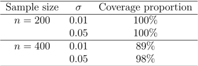
(17) Table 2: Simulation results showing observed coverage proportions for a nominal coverage of 95%.. Sample size σ Coverage proportion n = 200 0.01 100% 0.05 100% n = 400 0.01 89% 0.05 98% In order to evaluate the actual performance of the bootstrap confidence sets, a total number of 100 original samples of size 400 and 200 are generated, Si = {(Xi1 , Yi1 ), . . . , (Xin , Yin )} for i = 1, . . . , 100, and the corresponding prediction means are obtained, m(X)1 , . . . , m(X)100 . B = 100 bootstrap samples are taken from each sample Si and the corresponding bootstrap confidence sets at a 95% confidence level (nominal cover1 100 age) are constructed: CB0.95 , . . . , CB0.95 , or other words, the radii δ1 , . . . , δ100 are obtained. The observed coverage proportion of the theoretical prediction in such confidence regions is calculated as: p̂i =. i i , i = 1, . . . , 100} : m(X) ∈ CB0.95 card{CB0.95 . 100. (7). The results of the simulation study show that the method achieves good observed coverage proportions. Table 2 summarizes the numerical outputs of our simulation study. 6. Application to children’s body shapes The aim of this section is to show how the aforementioned algorithm can be used to predict the body shape of a child based on a small number of his or her anthropometric measurements and his or her age. The predicted shape could then be used to choose the most suitable size in a potential online sales application. There are multiple ways to perform this last step and all of them depend on the manufacturer. For instance, one possibility would be to calculate the Procrustes distance between the predicted shape and the shapes of the mannequins for each size. A randomly selected sample of 739 Spanish children aged from 3 to 12 was scanned using a Vitus Smart 3D body scanner from Human Solutions. Children were asked to wear a standard white garment in order to standardize 17.

(18) the measurements. From the 3D mesh, several anthropometric measures were calculated semi-automatically by combining automatic measurements based on geometric characteristic points with a manual review. In order to illustrate our procedure, two subsamples of our data set have been chosen. For both samples children over 7 years old were selected. The first sample consisted of 244 boys and the second consisted of 251 girls. The body shape of each child in our data-set was represented by 3075 3D landmarks, i. e. by a 3075 × 3 configuration matrix. Nine covariates were chosen in order to predict the shape of a child: age, height, bust circumference, waist circumference, hip circumference, right leg length, left leg length, right arm length, and left arm length. We choose these covariates because they are the most usual covariates asked in the online sales of wear. They are easy to measure in a child and well known by everybody. Figure 4 shows the prediction that was obtained when algorithm 1 was applied to predict the shape of a boy and the shape of a girl with the same covariates X0 . The following values for the covariates were employed: age = 9.5 years, height = 1385 mm, bust circumference = 717 mm, waist circumference = 643 mm, hip circumference = 770 mm, right leg length = 871 mm, left leg length = 872 mm, right arm length = 465 mm, and left arm length = 465 mm. Note how the two images are slightly different (mainly in the body trunk) despite the same values for the covariates and despite the short age of children in our sample. In this particular application, it would be desirable to have, in addition, a prediction of the children’s size. Although a kernel regression in the size and shape manifold could be applied, we can consider a rather simpler approach. Because size and shape could be considered independent, we can conduct a kernel shape regression and a univariate kernel regression separately for size given the above set of covariates. Then we join both predictions. In order to do a quantitative analysis of the effectiveness of the method a leave-out cross validation study is conducted. At each step of this study, a child is leaved out, and the Procrustes distance between their real shape and the predicted shape from the covariates is calculated. Because of the computational time just 10 % of children (chosen at random) have been leaved out, corresponding to 24 steps. The means of these prediction errors for different values of h and different numbers of iterations are shown in table 3. We can see that these prediction errors are larger for small numbers of iterations, and they reach the minimum and become stable after around 18.

(19) Table 3: Distances between real and predicted shapes for different values of h and number of iterations.. h 0.5 1.0 1.5 2.0 2.5 3.0. 100 0.0447 0.0448 0.0450 0.0451 0.0452 0.0453. Number of iterations 250 500 1000 0.0376 0.0351 0.0350 0.0373 0.0341 0.0335 0.0375 0.0342 0.0334 0.0377 0.0344 0.0336 0.0379 0.0346 0.0338 0.0381 0.0348 0.0341. 2000 0.0350 0.0334 0.0334 0.0335 0.0338 0.0340. 1000 iterations. In contrast, the prediction errors are quite robust against h-values, reaching the minimum for h = 2.0. In general, these errors are considered acceptable in our application, especially taking into account that just 8 anthropometrical measures plus the age are considered to predict the shape. In addition, unlike the simulated data set in the previous section, we must consider that all the shapes in this data set belong to children and, therefore, they show very similar shapes. The cross validation study is also used to test how reasonable are the bootstrap confidence regions. At each one of the 24 steps of the cross-validation study the confidence interval (determined by the corresponding δ-value) is obtained. Table 4 shows these values and the distances between the real and predicted shapes, as can we seen, distances are always smaller than δ-values. 7. Discussion In this paper we have proposed an approach that represents a novelty in terms of integrating concepts of statistical shape analysis and regression procedures. Although it is an important and common problem in real applications, papers on this subject are scarce in the literature. The main goal of this work was to show how to apply a general non-parametric regression method in manifold-valued data to the shape space based on landmarks. We also generalize the previous procedure to the case of multiple covariates and we propose bootstrap interval confidences for the predictions. A simulation study with simple objects was successfully conducted to validate the procedure. To illustrate our new methodology, it has been applied to a children body 19.

(20) Table 4: δ-values of the 95 % CI and distances between the real and predicted shape in 24 cases of the cross-validation study.. δ-value 0.037 0.032 0.035 0.029 0.056 0.033 0.037 0.035 0.029 0.045 0.046 0.025 0.034 0.046 0.029 0.039 0.036 0.036 0.029 0.057 0.025 0.029 0.033 0.024. Procrustes distance 0.036 0.029 0.034 0.027 0.053 0.030 0.036 0.032 0.027 0.043 0.042 0.024 0.032 0.044 0.027 0.036 0.034 0.034 0.027 0.055 0.024 0.027 0.031 0.023. 20.

(21) (a). (b). Figure 4: Shape predicted for (a) a boy (left) and (b) a girl (right) with the same covariates X0 = (9.5, 1385, 717, 643, 770, 871, 872, 465, 465). 21.

(22) data set with hundreds of subjects in order to predict the shape of a child given a small set of quantitative measures. The results obtained with this data set avail the feasibility of our new method. This regression method could be useful for the implementation of an online sales application. We used the R language and the shapes package in our implementations. Due to the large size and large dimensionality of our data set, the overall computational cost was too large. Thus, we improved the speed of some parts of certain routines of the aforementioned package to reduce the computational cost of the procedure. The new implementations were significantly faster than the original ones. Acknowledgements This paper has been partially supported by the grant DP I2013−47279− C2 − 1 − R from the Spanish Ministry of Economy and Competitiveness with FEDER funds. We would also like to thank the Biomechanics Institute of Valencia for providing us with the data set. Bhattacharya R, Patrangenaru V (2002) Nonparametric estimation of location and dispersion on riemannian manifolds. J Statist Plann Inference 108:23–35 Bhattacharya R, Patrangenaru V (2003) Large sample theory of intrinsic and extrinsic sample means on manifolds. The Annals of Statistics 31(1):1–29 Bookstein F (1978) Lecture notes in biomathematics. In: The measurement of biological shape and shape change, Springer-Verlag Davis BC, Fletcher PT, Bullitt E, Joshi S (2007) Population shape regression from random design data. In: Computer Vision, 2007. ICCV 2007. IEEE 11th International Conference on, IEEE, pp 1–7 Dryden IE, Mardia KV (1998) Statistical Shape Analysis. John Wiley & Sons, Chichester Dryden IL (2012) shapes package. R Foundation for Statistical Computing, Vienna, Austria, URL http://www.R-project.org, contributed package Fletcher PT, Zhang M (2016) Probabilistic geodesic models for regression and dimensionality reduction on riemannian manifolds. In: Riemannian Computing in Computer Vision, Springer, pp 101–121 22.

(23) Fletcher T (2011) Geodesic regression on riemannian manifolds. In: Proceedings of the Third International Workshop on Mathematical Foundations of Computational Anatomy-Geometrical and Statistical Methods for Modelling Biological Shape Variability, pp 75–86 Fréchet M (1948) Les éléments aléatoires de nature quelconque dans un espace distancié. Annales de l’Institut Henri Poincare Probabilités et Statistiques 10(4):215–310 González-Rodrı́gez G, Trutschnig W, Colubi A (2009) Confidence regions for the mean of a fuzzy random variable. In: Carvalho JP, Dubois D, Kaymak U, J M da Costa Sousa P Eds Lisbon (eds) IFSA-EUSFLAT, pp 1433–1438 Goodall C (1991) Procrustes methods in the statistical analysis of shape. Journal of the Royal Statistical Society Series B (Methodological) pp 285– 339 Härdle WK, Müller M, Sperlich S, Werwatz A (2012) Nonparametric and semiparametric models. Springer Science & Business Media Jupp PE, Kent JT (1987) Fitting smooth paths to speherical data. Applied Statistics pp 34–46 Karcher H (1977) Riemannian center of mass and mollifier smoothing. Communications on pure and applied mathematics 30(5):509–541 Kendall D (1984) Shape manifolds, procrustean metrics, and complex projective spaces. London Math Soc 16:81–121 Kendall D, Barden D, Carne T, Le H (2009a) Shape and shape theory, vol 500. John Wiley & Sons Kendall DG, Barden D, Carne T, Le H (2009b) Shape and shape theory. John Wiley & Sons, Chichester Kendall WS (1990) Probability, convexity, and harmonic maps with small image i: uniqueness and fine existence. Proceedings of the London Mathematical Society 3(2):371–406 Kim H, Adluru N, Collins M, Chung M, Bendlin B, Johnson S, Davidson R, Singh V (2014) Multivariate general linear models (mglm) on riemannian 23.

(24) manifolds with applications to statistical analysis of diffusion weighted images. In: Proceedings of the IEEE Conference on Computer Vision and Pattern Recognition, pp 2705–2712 Kobayashi S, Nomizu K (1969) Foundations of Differential Geometry. Vol. II. Wiley, Chichester Mammen E (2000) Resampling methods for nonparametric regression. In: Smoothing and Regression: Approaches, Computation, and Application, Wiley Online Library, pp 425–450 Mardia KV, Jupp PE (2009) Directional statistics, vol 494. John Wiley & Sons Nadaraya EA (1964) On estimating regression. Theory of Probability & Its Applications 9(1):141–142 Pennec X (2006) Intrinsic statistics on riemannian manifolds: Basic tools for geometric measurements. Journal of Mathematical Imaging and Vision 25(1):127–154 R Development Core Team (2014) R: A Language and Environment for Statistical Computing. R Foundation for Statistical Computing, Vienna, Austria, URL http://www.R-project.org, ISBN 3-900051-07-0 Shi X, Styner M, Lieberman J, Ibrahim JG, Lin W, Zhu H (2009) Intrinsic regression models for manifold-valued data. In: Medical Image Computing and Computer-Assisted Intervention–MICCAI 2009, pp 192–199 Small C (1996) The statistical theory of shape. Springer New York Stoyan LA, Stoyan H (1995) Fractals, Random Shapes and Point Fields. John Wiley and Sons, Chichester Vinué G, Simó A, Alemany S (2014) The k-means algorithm for 3D shapes with an application to apparel design. Advances in Data Analysis and Classification 10(1):103–132 Woods R (2003) Characterizing volume and surface deformations in an atlas framework: theory, applications, and implementation. NeuroImage 18:769– 788 24.

(25)