Novel Method to Improve the Signal to Noise Ratio in the Far-field Results Obtained from Planar Near Field Measurements.

(1)

Novel method to improve the signal-to-noise ratio in the far-field results obtained from planar

near-field measurements

F. J. Cano-Fácila

1

, S. Burgos

2

, M. Sierra-Castañer

1

, J. L. Besada

1

Universidad Politécnica de Madrid (UPM). E.T.S.I. de Telecomunicación

Ciudad Universitaria, 28040 Madrid, Spain

2

Antenna Systems Solutions, S.L. (ASYSOL), c/ Manuel Cortina 12, 28010, Madrid, Spain

E-mail: [email protected], [email protected], [email protected],

[email protected]

ABSTRACT

A method to reduce the noise power in far-field pattern without modifying the desired signal is proposed. Therefore, an important signal-to-noise ratio improvement may be achieved. The method is used when the antenna measurement is performed in planar near-field, where the recorded data are assumed to be corrupted with white Gaussian and space-stationary noise, because of the receiver additive noise. Back-propagating the measured field from the scan plane to the antenna under test (AUT) plane, the noise remains white Gaussian and space-stationary, whereas the desired field is theoretically concentrated in the aperture antenna. Thanks to this fact, a spatial filtering may be applied, cancelling the field which is located out of the AUT dimensions and which is only composed by noise. Next, a planar field to far-field transformation is carried out, achieving a great improvement compared to the pattern obtained directly from the measurement. To verify the effectiveness of the method, two examples will be presented using both simulated and measured near-field data.

Keywords: Anechoic chamber, antenna measurements,

back-propagation, filtering, Gaussian noise.

1. Introduction

Near-field measurements have become one of the most commonly employed techniques to obtain antenna radiation patterns. In contrast to conventional far-field ranges, the distance between the antenna under test (AUT) and the probe is reduced, and unwanted contributions from reflections or diffraction from the environment are largely suppressed in the anechoic chambers in which these measurements are typically performed. Moreover, accurate far-field results can be obtained from near-field data by using either a modal expansion method [1], [2] or an equivalent currents reconstruction method [3], [4]. These techniques yield far-field results that are in many cases more accurate than the obtained in a far-field range. Nevertheless, as in all

measurements, there are always sources of error that must be taken into account in near-field AUT measurements. References [5]-[10] are examples of studies that examine the relationships between the measurement errors and their effects on the far-field using mathematical analyses, simulations, or measurement tests. The results obtained in these studies can be used to estimate the impact of a particular error or a combination of errors on the far-field pattern. In addition, the results can be used to deduce the maximum admissible near-field error for a given level of accuracy in the far-field or to assess the accuracy of a near-field range [11].

Random noise is one of the errors that limits the accuracy of far-field results, particularly, when measuring a low-sidelobe or a high-performance antenna. Some comprehensive studies for random noise in near-field measurements have already been presented. For the planar system, two independent analyses with similar results have been proposed in [12], [13]. Both of them start with random errors in the planar near-field and obtain expressions that represent the signal-to-noise ratio in the far-field as a function of the noise power in the near-field. A similar study for cylindrical near-field measurements was carried out in [14], [15]. These latter publications derived an expression relating the noise power in the near-field and far-field. The cylindrical case was also discussed in [16], which investigated the improvement of the signal-to-noise ratio achieved through the cylindrical near-field to far-field transformation.

(2)

about the presented method can be found in [19].

This paper is organized as follows. Section 2 gives an overview of the back-propagation process to obtain the field at the AUT plane from the measured field. The effect of the back-propagation process on the random noise is also analyzed in this section. Section 3 describes the method implemented to improve the signal-to-noise ratio. Section 4 presents two numerical results to analyze the effectiveness of the algorithm. Finally, conclusions are discussed in section 5.

2. Back-propagation of the planar near-field

As previously stated, the objective of this paper is to mitigate the undesired effects of random noise when the measurement is performed in planar near-field. This noise mitigation is accomplished by means of filtering before obtaining the far-field results. Because all the measured data are always noise corrupted, filtering cannot be applied to this initial information and a new data representation that allows for noise filtering without cancelling out the desired information is needed. For this, once the planar near-field measurement has been performed, the field at the AUT plane (reconstructed field) is computed. Because, the desired contribution is theoretically located inside the dimensions of the AUT, filtering can be applied to cancel the outside contribution due to noise.

2.1. Theoretical description of the transformation

Because the scan plane and the AUT plane are parallel, an easy transformation from one plane to the other can be performed using field back-propagation [20], [21]. Assuming that the normal axis to both planes is the z-axis and that the distance between them is d, the measured near-field components are Emeas x_,

x y d, ,

and

, , ,

meas y

E x y d . In addition, the plane wave spectrum

(PWS) components referenced to the scan plane,

, ,

x x y

P k k d and P k k dy

x, y,

, are calculated as follows

,

, 1

, , , ,

2 1

, , , ,

2

x y

j k x k y x x y meas x

j k x k y y x y meas y

P k k d E x y d e dxdy P k k d E x y d e dxdy

S

³³

(1)

The next step to calculate the reconstructed field is to reference the last quantities given by (1) to the AUT plane. Each plane wave is multiplied by a term that depends on the distance between planes as well as the longitudinal component of the propagation vector,

2 2 2 0

z x y

k k k k .

, , 0 , ,

z

jk d x x y x x y

jk d y x y y x y P k k P k k d e P k k P k k d e

(2)

Finally, using the inverse expression of (1), the electric-field components over the AUT plane,

, , , 0

ap x

E x y and Eap y_,

x y, , 0

, can be computed.

,

1

, , 0 , , 0

2 1

, , 0 , , 0

2

x y

j k x k y

ap x x x y x y

j k x k y

ap y y x y x y

E x y P k k e dk dk E x y P k k e dk dk

S

³³

(3)

2.2. Noise analysis in the back-propagation process

After reviewing the theory behind the planar near-field to reconstructed field transformation, an analysis to assess the noise behavior and to obtain its statistical parameters was carried out. In the analysis, a complex white Gaussian and space-stationary noise was considered. Its mean and variance were assumed to be zero and 2

nf

V , respectively. Because all the expressions are linear for the back-propagation process, the analysis is performed by considering only the noise. In addition, the expressions and the noise are the same for both electric-field polarizations. As a result, the study is developed for a generic case.

Using planar near-field data containing only noise and applying the discrete version of (1), the PWS referenced to the scan plane due to the noise can be obtained.

1

, , , ,

2

x i y i

M

j k x k y x y nf i i

i x y

N k k d n x y d e

S

' '

_¦

(4)

where nnf

x y di, i,

represents the planar near-field,

x, y,

N k k d is the PWS referenced to the scan plane, 'x

and _'_y symbolize the sample spacing in the x- and y -directions, and M is the total number of planar near-field samples. Because noise is an independent random variable at each measurement point, the PWS obtained from (4) is also modeled as Gaussian and space-stationarity noise with zero mean. The variance is determined as (5) indicated.

2 *

2 2

0, 0 , , , ,

2

N N x y x y

nf

R E N k k d N k k d x y

M

V

V S

ª º

¬ ¼

' '

§ ·

¨ ¸

© ¹

(3)

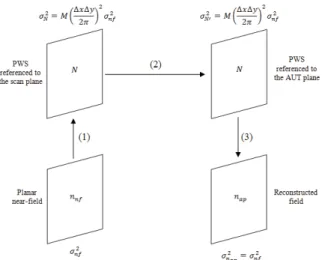
Figure 1 – Statistical properties of noise in the field back-propagation

The next step in the transformation process is reference previous PWS to the AUT plane. To do this, the PWS is multiplied by a complex factor of unity amplitude, as shown (6). The resulting quantity is also another Gaussian noise with the same statistical properties.

, , 0 , ,

jk dz

x y x y

N k k N k k d e (6)

Finally, the reconstructed field is obtained by using the discrete version of (3).

, ,

, , , , ,

, ,

1

1 1

, , 0 , , 0

2

, ,

2 2

k

x m y m

k

x m i y m i x m y m z m

M

j k x k y

x y

ap x m y m

m

M M

j k x k y j k x k y

jk d

x y

nf i i

m i

k k

n x y N k k e

k k x y

e n x y d e e

S

S S

' '

' ' ' '

¦

(7)

where nap

x y, , 0

is the field over the AUT plane, 'kx and y

k

' represent the spectral steps in the kx- and ky

-directions, and M_k stands for the total number of spectral samples. The total number of spectral samples is equal to M because, the last summations in (4), (7) are evaluated using the FFT algorithm.

From (7), it is deduced that the field at each point of the reconstructed plane is also a Gaussian random variable with zero mean and variance calculated as in (5), i.e., by determining the autocorrelation in (0,0).

2 *

2 2

2 2 2 2

0, 0 , , 0 , , 0

2 2

ap ap

x y

n n ap ap

y x

nf nf

R E n x y n x y

yM xM

k k

V

V V

S S

ª º

¬ ¼

'

§ ·

'

§ · _' _'

¨ ¸

(8)

Figure 2 – Regions of interest in the reconstructed domain

where the following relationships have been taken into account:

k

M M (9)

x y

M M M (10)

2 2

;

x y

k k

xM yM

S S

' '

' ' (11)

where M_x and M_y represent the number of planar near-field samples in the x- and y-directions.

From the previous analysis, it can be seen that, for planar near-field noise with the aforementioned statistical characteristics, the noise both in the PWS and in the reconstructed field is a complex, stationary, white Gaussian noise, with zero mean and variance given by (5) and (8), respectively, as shown Figure 1.

3. Description of the method

As mentioned before, the main purpose of the proposed method is to reduce the far-field noise power obtained in a planar near-field measurement. However, noise reduction cannot be achieved at the input because both the noise and the desired contribution are distributed over the whole measurement surface. For this reason, a field transformation is required to filter out a portion of the noise without modifying the desired signal. This paper presents a method that performs back-propagation of the field from the scan plane to the AUT surface. The steps of the method are indicated below:

x Perform a planar near-field measurement. x Obtain the PWS referenced to the scan plane. x Back-propagate the PWS from the scan plane to

the AUT plane.

(4)

x Filter the portion of noise located beyond the AUT dimensions.

x Calculate a new PWS with less noise power.

After presenting all the points of the proposed method, we analyze the signal-to-noise ratio improvement which can be achieved. The definition of filtering employed in the method appears in (12).

A 1

T A

1 ,

,

0 , x y F x y

x y Z Z Z ° ® °¯ (12)

where _Z_T and _Z_A represent the reconstructed region and

the AUT region depicted in Figure 2. In Figure 2, D_x and

y

D are the x- and y-dimensions of the reconstructed surface. A_x and A_y represent the maximum length of the AUT in each direction.

As shown below, the variation of the maximum signal level in the PWS due to filtering is negligible. As a result, the signal-to-noise ratio improvement remains equal to the noise reduction. The noise power in the PWS for any kind of filtering applied is given by (5). Thus, the only unknown quantity needed to specify the improvement is the variance of the noise in the PWS obtained after spatial filtering. This new PWS is determined as follows

, , , , , 1 1 2

1 1 1

' , , 0 , , , 0

2

2 2

· , ,

x r y r

k A

x m i y m i x m r y m r x r y r z m

M

j k x k y

x y r r ap r r

r

x y

M M M

j k x k y j k x k y j k x k y

jk d

nf i i

r m i

x y

N k k F x y n x y e

k k x y

e n x y d e e e

¦

¦ ¦

¦

(13)

The noise power of this final quantity, denoted as 2 '

N

V , can be calculated as (14) indicates.

2 * ' ' 2 2 2

2 2 2

2

0, 0 ' , , 0 ' , , 0

2 2 2

2

A

x y

A

N N x y x y

y x

nf

nf x y

R E N k k N k k

M yM

xM x y

M k k

M S x y M D D Z Z V V

S S S

S_Z is the area of Z_A. Therefore, the signal-to-noise ratio improvement achieved with the proposed spatial filtering method can be calculated using (5) and (14).

Figure 3 – Simulated near-field. Comparison between the reference PWS, the PWS with noise and the PWS

after the noise filtering in II = 90º plane.

2 ' , 2 A x y SF N SF th WF N S D D SNR SNR S

SNR S_Z

V

' (15)

where SNR_SF and SNR_WF are the signal-to-noise ratios after spatial filtering and without filtering and 'SNR_{SF th}_, symbolizes the theoretical increase in the signal-to-noise ratio due to spatial filtering.

In this section, the desired field is assumed to be concentrated on the AUT region. Nevertheless, this assumption is not completely correct. A small field contribution always exists outside the AUT. The cancellation of this contribution may introduce a significant error, mainly in the sidelobes, in the final PWS. To avoid this negative effect, spatial filtering over a larger area must be employed to account for all of the desired data.

4. Numerical results

To validate the proposed method, two different examples are presented. The first one takes as input data the values of a simulation of a planar acquisition. The last one uses information of an actual measurement in the planar near-field range of the Technical University of Madrid (UPM).

4.1. Simulation data

In this first example, a simulation that considers both noise and the contribution of the AUT is presented. The AUT is composed of 20 x 20 infinitesimal dipoles with a uniform excitation. The separation between the dipoles is

(5)

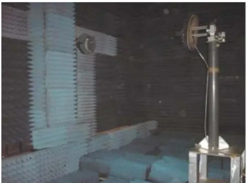
Figure 4 – Experimental measurement of a pyramidal horn antenna in a planar near-field range

of the infinitesimal dipole array has been simulated, taking into account all previous specifications, Gaussian noise with 25 dB less power than the maximum of the simulated data is added. Next, the proposed method is applied. Figure 3 shows a cut of the radiation pattern, seeing that a great improvement is achieved after filtering a portion of noise in the reconstructed field. The improvement can be calculated by applying (15) and is equal to 20 dB.

4.2. Measured planar near-field data

In another example that uses the data from an actual measurement, data were obtained by using the planar-range measurement system in the anechoic chamber at the Technical University of Madrid (UPM). For the experiment, the probe and the AUT consisted of a corrugated conical-horn antenna and a 5 cm × 7 cm pyramidal-horn antenna. The antennas were separated by 1.57 m. Once both antennas were mounted onto positioners (see Fig. 4), a measurement over a 2.4 m×2.4 m acquisition plane with a spatial sampling equal to 0.43 λ 13 GHz

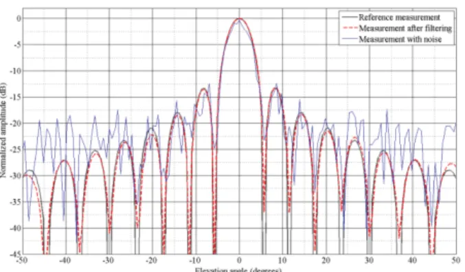
was recorded. Gaussian noise with 30 dB less power than the maximum of the acquired data was added computationally. As in the preceding example, after obtaining the corrupted data, the method to improve the signal-to-noise ratio was employed. In this case, there is a large truncation error, so a filtering window larger than the AUT dimensions was required (0.3 m x 0.3 m). The improvement achieved with this filtering is equal to 18.06 dB. Figure 5 depicts a cut of the radiation pattern where it is possible to see that improvement.

5. CONCLUSIONS

In this paper, we have presented a simple and efficient method to improve the signal-to-noise ratio in far-field results obtained from planar near-field measurements. Firstly, a statistical study of the noise was performed. Next, the method was exposed and then was validated with two numerical results. As mentioned before, because

Figure 5 – Experimental measurement in planar near-field. Comparison between the reference PWS,

the PWS with noise and the PWS after the noise filtering in II = 90º plane.

the method can only be applied in planar near-field measurements, there will be a truncation error which may significantly extend the reconstructed field beyond the AUT dimensions. Therefore, an adaptive filtering window has to be used.

6. REFERENCES

[1] A. D. Yaghjian, “An overview of near-field antenna measurements,” IEEE Trans. Antennas Propagat., vol. AP-34, No. 1, pp. 30-44, Jan., 1986.

[2] R. C. Johnson, H. A. Ecker, and J. S. Hollis, “Determination of far-field antenna patterns from near-field measurements,” Proc. IEEE, vol. 61, No. 12, pp. 1668-1694, Dec., 1973.

[3] P. Petre and T. K. Sarkar, “Planar near-field to far-field transformation using an equivalent magnetic current approach,” IEEE Trans. Antennas Propagat., vol. 40, No. 11, pp. 1348-1356, Nov., 1992.

[4] T. K. Sarkar and A. Taaghol, “Near-field to near/far-field transformation for arbitrary near-near/far-field geometry utilizing an equivalent electric current and MoM,” IEEE Trans. Antennas Propagat., vol. 47, No. 3, pp. 566-573, Mar., 1999.

[5] A. C. Newell, “Error analysis techniques for planar near-field measurements,” IEEE Trans. Antennas Propagat., vol. 36, No. 6, pp. 754-768, Jun., 1988. [6] L. A. Muth, “Displacement errors in antenna

near-field measurements and their effect on the far-near-field,” IEEE Trans. Antennas Propagat., vol. 36, No. 5, pp. 581-591, May, 1988.

[7] H. Hojo and Y. Rahmat-Samii, “Error analysis for bi-polar near-field measurement technique,” in Proc. 1991 IEEE/AP-S Int. Symp., London, ON, Jun. 24-28, 1991, pp. 1442-1445.

(6)

[9] M. H. Francis and R. C. Wittman, “Sources of uncertainty for near-field measurements,” in Proc. 2007 IEEE/The Second European Conference on Antennas Propagat. (EuCAP 2007), Edinburgh, Nov. 11-16, 2007, pp. 1-3.

[10]J. E. Hansen, “Error analysis of spherical near-field measurements” in Spherical Near-Field Antenna Measurements, Peter Peregrinus Ltd., London, UK, 1988, ch. 6, pp. 216-254.

[11]E. B. Joy, “Near-field range qualification methodology,” IEEE Trans. Antennas Propagat., vol. 36, No. 6, pp. 836-844, Jun., 1988.

[12]A. C. Newell and C. F. Stubenrauch, “Effect of random errors in planar near-field measurement,” IEEE Trans. Antennas Propagat., vol. 36, No. 6, pp. 769-773, Jun., 1988.

[13]J. B. Hoffman and K. R. Grimm, “Far-field uncertainty due to random near-field measurement error,” IEEE Trans. Antennas Propagat., vol. 36, No. 6, pp. 774-780, Jun., 1988.

[14]J. Romeu, L. Jofre, and A. Cardama, “Far-field errors due to random noise in cylindrical near-field measurements,” IEEE Trans. Antennas Propagat., vol. 40, No. 1, pp. 79-84, Jan., 1992.

[15]J. Romeu and L. Jofre, “Effect of random errors in cylindrical near-field measurements,” in Proc. 1991 IEEE/AP-S Int. Symp., London, ON, Jun. 24-28, 1991, pp. 1450-1453.

[16]J. Romeu, L. Jofre, and A. Cardama, “An approximate expression to estimate signal-to-noise ratio improvement in cylindrical near-field measurements,” IEEE Trans. Antennas Propagat., vol. 42, No. 7, pp. 1007-1010, Jul., 1994.

[17]P. Koivisto, “Reduction of errors in antenna radiation patterns using optimally truncated spherical wave expansion,” Progress In Electromagnetic Research, vol. pier-47, pp. 313-333, 2004.

[18]L. J. Foged and M. Faliero, “Random noise in spherical near-field systems,” in Proc. 2009 Antenna Meaurement. Techniques Assoc., AMTA, Salt Lake City, UT, Nov. 1-6, 2009, pp. 135-138.

[19]F. J. Cano-Fácila, S. Burgos and M. Sierra-Castañer, “An efficient algorithm to improve the signal to noise ratio in planar near-field measurements,” IEEE Trans. Antennas Propagat., submitted for publication.

[20]J. J. H. Wang, “An examination of the theory and practices of planar near-field measurement,” IEEE Trans. Antennas Propagat., vol. 36, No. 6, pp. 746-753, Jun., 1988.

[21]E. Martini, O. Breinbjerg, and S. Maci, “Reduction of truncation errors in planar near-field aperture antenna measurements using the Gerchberg-Papoulis algorithm,” IEEE Trans. Antennas Propagat., vol. 56, No. 11, pp. 3485-3493, Nov., 2008.

7. ACKNOWLEDGMENTS