Evolution Models for Dynamic Networks
Pedro J. Zufiria and Iker Barriales-Valbuena
Abstract—This paper proposes a mathematical framework for modelling the evolution of dynamic networks. Such framework allows the time analysis of the relationship between the dynamic laws and the network characterizing features (degree distribu-tion, clustering coefficient, controllability indexes, etc.) providing new insight on the network properties. The framework also allows to relate and generalize existing inference procedures for modelling real world time evolving complex systems.
Keywords—Complex Networks, Dynamics, Stochastic Mod-elling, Estimation
I. INTRODUCTION
I
N the last decade the modelling of complex networks [1], [2], [3] has become a very active research field since many different complex systems share some essential common features which can be gathered in a network model [4]. Although network elements can represent very different entities depending on the phenomenon being analyzed, still some common characteristics seem to be ubiquitous in many models. For instance, common patterns usually appear in social networks ([5]), biology networks ([6]), technological networks ([7], [8]) or information networks ([9], [10]).The common features of these (usually very large) networks rely on statistical properties; hence, random graph models have been successfully employed for characterizing such networks. Starting from the seminal model [11] which served as a baseline for comparative purposes, several more sophisticated models have been proposed to explain the behavior of complex networks.
The characterization of complex networks can be addressed by considering them as either static or dynamic entities. The most frequent static perspective is grounded on constructing a probability space (i.e., a probability measure on the space of possible networks); this probability model allows for a compact network characterization and it can be employed for several purposes (e.g., link/edge detection). Network evolution models gather information along time and they are (often im-plicitly) grounded on the construction of a stochastic process on the space of possible networks. They can be very useful for network completion or prediction. Here we formalize this perspective.
II. GENERATION MODELS. PROBABILITY SPACE
The most simple network generation models define a prob-ability space associated with the set of all possible networks.
Such space can be denoted by (Q,Y¡g,P), where Q is the sample space (or set of possible networks), Eg corresponds with the set of all possible events, and P is a probability measure on Eg.
A. Sample space
In order to construct Q one has to define the set of variables which characterize a given network (the simplest model considers G := {V, E}, where V is a set of vertices and E is a set of edges). Here, two basic situations can be encountered: V is a fixed set which does not change with time. Then \V\ = n and E is the set of all possible edges, with cardinal \E\ = (™). Hence, in this case a network G¿ is defined by its corresponding set Ei c E, and we have \Q\ = 2lBL Alternatively, Vt may change with time. In such
case, we can consider V to represent the maximum set of edges over time, so that Vt c V. Then, all Vt c V (with \Vt\ = nt)
has an associated set of possible edges Et, which satisfies
|St| = ("2). Therefore, the set of all possible networks over time must gather all these possibilities and will satisfy l^l = E v , c v2^l= 0 ( 2 l£l ) .
B. Set of events Eg
Since Q is considered to be a finite set, a natural (and the largest) a-algebra (set of events) can be defined as Eg = Power set of Q. Note that any property V defined in relation to networks (e.g., being connected, containing triangles, having a given degree k, etc.) is associated with a given element of the set of events {Q-p e Eg) or a subset of the sample space (9r c G).
C. Probability measure
Again, since Q is finite, it suffices to define P(G), Ve? e Q, all the elementary events. For a fixed set of nodes V, the random network is defined by a set of \E\ random variables (the edge indicators of the network). In general \Q\ = 2^1 may be too large for an explicit definition of each P{G); hence, manageable laws are desirable for defining P, based on simplifying or regularity assumptions.
Typically, hypothesis such as distribution uniformity or independence among some variables (considered to represent known properties of the phenomenon to be modelled) are employed allowing for an easier construction or definition of P.
different P measure or distribution). Hence, expressions such as "ER network" should be qualified to "ER distribution-based generated network".
1) Erdos-Renyi (ER) procedure [12]: This procedure is grounded on a uniformity assumption. It considers Q as the set of networks with n vertices, and it defines:
P(O) = i ^ VGegn (1)
where Qm is the set of networks having m edges, whose size
is given by \Qm\ = ( ^ ' ) , where \E\ = (™).
Networks created (as a sample) following the ER procedure are usually called ER networks.
2) Gilbert model [13]: This network model considers that each of the edge indicators is a Bernoulli random variable with probability p (with same value of p for each link). The number of edges in the networks generated by this model follows a Binomial distribution with parameters \E\ and p. Note that the conditional distribution for a fixed number of edges m is uniform, thus being equivalent to the ER model.
3) Range dependent random graphs [14]: These models also consider that each edge e¿ indicator is a Bernoulli random variable with probability pi = /(r¿), where r¿ is the range (a distance measure) between the pair of nodes linked by e¿.
4) Kronecker graphs [15]: These models are based on the generation of matrices via Kronecker products, being math-ematically tractable while generating networks with desired structural properties (heavy tail distributions, densification, etc.).
5) Exponential Random Graphs Models (ERGMs) [16]: Random Networks can be generally modelled by:
P{G) = exp(0*s(G)) £G'e £ ?e x p ( 0 'S( G ' ) ) '
VGeg (2)
where 9 is a vector of parameters and s is a vector of features (sufficient statistics). In general, for any type of random network distribution, the size of s could be huge, each component gathering information associated with any arbitrary subset of nodes in the network.
ERGM models are grounded on some simplifying assump-tions which allow for an easy definition or characterization of P via conditional probabilities. This fact guarantees that the definition of the distribution only requires a reduced set { s i , . . . , sfc} of features, which allows for a good practical
applicability.
a) Markov graphs [17]: The term Markov Graph defines a sub-family of distributions (or measures) for graphs with even stronger simplifying conditional independence properties. A random graph is a Markov Graph if non-incident edges (i.e., edges between disjoint pairs of nodes) are independent conditional on the rest of the graph. The Markov Graph assumption guarantees that the the set { si ;. . . , sk} of features
only needs to consider triangles and A;-stars. (Note that the term Markov Network or Markov Field is also employed when considering dependence graphs for random variables; here we use the term to refer to families of distributions on networks.)
D. Inference of Random Network Models
If we consider a given network to be a sample from a Random Network model, strong assumptions (i.e. inductive bias) must be imposed for carrying out a model inference from that single sample (network). (A similar circumstance shows up when addressing parameter estimation for vector joint distributions by making use of a single or few vector samples; such estimation can be carried out if strong (e.g. Markov type) simplifying assumptions are assumed in the model. In addition, sometimes only partial knowledge of the network (sub-network) is available.
1) Inference of Markov Graphs: The Markov Graph model assumption provides a strong inductive bias which also allows for model inference from a single sample (network). Usually, the inference procedure to obtain P is carried out as follows: the ERGM structure is assumed on P and, given a (sample) network and a set s of chosen features (number of links, number of triangles, etc.), a maximum likelihood estimate for 6 is constructed. The resulting network distribution model max-imizes the likelihood of the sample network and all networks with the same features s [18]. This fundamental procedure leads to a whole family of models [19]. Nevertheless, the standard likelihood techniques for the Markov models are not immediately applicable because of the complicated functional dependence of the normalizing constant c on the parameters. Hence, practical estimation procedures need to perform a sampling in the network (which could also be interpreted as analyzing an appropriate sub-network) via, for instance, Gibbs sampling [20], pseudo-likelihood techniques [21], or stochastic approximation based procedures [22], [23].
III. EVOLUTION MODELS. STOCHASTIC PROCESSES
In this section we model evolution networks as Markovian stochastic processes. These processes {Gt, t eT} satisfy the
condition
P{Gt = G/Fs) = P{Gt = G/Gs (3)
Among these processes, we can select a special class of stochastic dynamical systems:
Gt+i = F(Gt,wt), (4)
where the random process wt has an associated measurable
space (W, W) adapted to the filtration T so that VA e W, it satisfies P{wt = A/Fs) = P{wt = A/ws). In general, A
defines a property on W.
In the following, we propose stochastic dynamical systems for characterizing evolving networks.
A. State space and time evolution. Evolution equations The state space comes from the definition of the set of all possible networks Q, and the (discrete) time variable can be defined upon two natural options:
. Define time instants where the probability space (i.e., the filtration Ft) does change.
Considering the already defined state space structure, the
general evolution formulation of (4) can be broken down into: E, i + i
Vt+1 = Fv(yt,Et,wt),
Et+1 = FE(Vt,Et,wt),
where wt is a stochastic process.
(5) (6)
B. Generation processes associated with ER and Gilbert mod-els
1) Generation process for Erdos-Renyi distribution: The ER model basic generating procedure is defined as follows:
• Fix a set of vertices V (with \V\ = n), so that Q is determined by the set of all possible edges E.
. Define the subset of networks with exactly m edges, Qm c Q.
• Randomly select a network from Qm, based on the
probability distribution described in (1).
Alternatively, one can define a growing dynamic process that characterizes the usual "construction" procedure whose final outcome can be interpreted as a sample from a network following the ER distribution:
. V fixed (i.e., Vt = V, Vt),
. £o = 0,
. Et+1 = FE(Vt,Et,wt) = Et U {et}, where et is
ran-domly selected among the elements of E \ Et, according
to a uniform distribution.
For t = m, Em has m elements, Gm G Qm and P{Gm =
G) = TJ—^ , VG G Qm (uniform), corresponding to a network
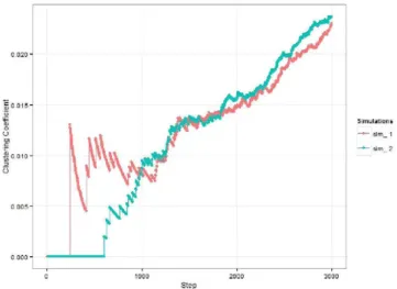
which follows the Erdos-Renyi distribution. In Figure 1 this generation model has been simulated and the evolution of the network clustering coefficient along time has been computed. As expected, as time increases such coefficient tends to linearly increase with time.
Fig. 1. Clustering time evolution in ER model generation procedure.
2) Generation process for Gilbert distribution: The follow-ing process can also be related to the Gilbert network model:
• V fixed, . £o = 0,
EtU {et}, with prob. p,
Et, with prob. I —p.
where e¡ corresponds to the t-th element of E = {e\,...e\E\} (depending on the relevance of node
or-dering one may also employ any alternative permutation of this set).
For a given t, the distribution associated with graph Gt is
characterized as follows:
• |St| follows a binomial distribution B{t,p) (hence, E[\Et\]=t-p).
. P(Gt = G) = _ P{\Et\=m) vc? G g„ (uniform), m G
) follows an ER { 0 , . . . ,t} (Note that P{Gt/\Et\ =
distribution with parameter m.)
Note that this process is defined for t G { 0 , 1 , . . . , \E\}. An alternative associated process can be defined, for instance, by randomly selecting et G E \ Et, which would eventually end
up converging to a fully connected network.
C. Growing processes
Network growth has been analyzed in the last two decades as a mechanism for explaining some network special features, such as long tail degree distributions. Many growing models with given properties have been proposed in the literature [9], [24], [25]. All these models can be stated in the following framework:
. G0 = (V0, E0), starting network,
• Vf+1 = VtU{vt}, where vt G V\Vt is chosen (depending
on the relevance of node ordering, this selection can be done at random).
• Et+í = Et U AEt,
where AEt = {e\,... elt*} C E\ Et is chosen following
a given law C.
Law C for selecting AEt determines the specific model, and
it can be formalized via: • F = (FV,FE),
• Property A associated with the filtration Tt (i.e, C
depends on wt G A or wt £ A).
In Figure 2 the time evolution of the clustering coefficient for a BA model is presented. As expected, as time increases such coefficient tends to decrease [26], [27].
D. Evolution processes
In the last decade, several specific evolving models which include addition and deletion of nodes and links have been proposed in the literature. In [28] the time evolution of the degree distribution is computed, and in [29] a model based on the range dependent model [14] is proposed. Alternatively, the ERGMs models have been extended to the TERGMs (Time Exponential Random Graph Models): in [30] the transition probabilities are modelled based on a temporal dependence Markov assumption, whereas in [31] this type of models are refined to separately characterize link formation and link duration phenomena. Finally, a more general form gathering longer time dependencies is presented in [32].
r
r
D . D D -
t
1333 2000 2333 ¿333 Step
Í . 3
-—
—
-—
—
300 600 1200 1500 1800 2100 2400 2700 3000
Step
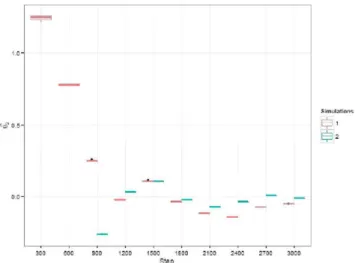
Fig. 2. Clustering time evolution in BA model generation procedure. Fig. 3. Estimated ERGM 6\ time evolution in ER model procedure.
Go
14+1 =
04
E, i + i
E0) starting network,
VtUAVt, AVteV\Vt
AVt G vt
AEt £ E\Et
AEt G Et
V \ AVt,
Et U AEt,
Et \ AEt,
(following C) (following C) (following C) (following C) which means that, in each iteration, the network can grow or diminish depending on C (i.e., F and wt).
Many different features can be analyzed for a given model using stochastic processes techniques. The time evolution analysis of relevant features (clustering coefficient, degree distribution, controllability indexes, etc.), can shed light on the relationship among them.
+
-E. Inference in evolution processes
The presented analytical framework allows to relate differ-ent inference procedures used for static networks and evolution models. The inference methods to construct an ERGM for the probability space in a network model make use of a single network as a sample; on the other hand, evolution models are built from a sample of an evolving process (knowledge of the network over a period of time). TERGMs are aimed to infer such time evolution models.
An interesting approach for time evolution analysis is the characterization of model parameter estimates along time. This information may be helpful for comparison between models and prediction purposes. In the following we apply this characterization procedure to the ER and BA models. Figures 3 and 4 show the time evolution of #i (related to density) and §2 (related to number of triangles) coefficients estimated via an ERGM for an ER generation process. Note that this evolution matches with the known evolution of density and number of triangles in the ER generation process.
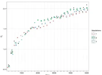
Figures 5 and 6 show the time evolution of 6\ and §2 coefficients estimated via an ERGM for a BA generation process. These results can be employed for prediction even in an increasing number of nodes scenario.
Fig. 4. Estimated ERGM 82 time evolution in ER model procedure.
•Am
Fig. 6. Estimated ERGM θˆ2 time evolution in BA model generation
procedure.
I V . CONCLUDING REMARKS A N D FUTURE WORK
A mathematical framework has been proposed for charac-terizing time evolving networks. Such framework allows the study of many different features, whose time evolution analysis may provide new insight on network properties. It also allows to relate inference procedures used for static networks and evolution models. The simulations illustrate the possibility of predicting model evolution even in scenarios where the number of nodes increases.
Future work is focused on the time evolution analysis of the relationship between the type of evolution laws, the computed inference models and network characterizing features (clus-tering coefficient, degree distribution, controllability indexes, etc.). The application of this inference techniques in evolution processes may provide a way to compute models applicable to real world time evolving complex systems.
REFERENCES
[1] Albert-La´szlo´ Baraba´si and Jennifer Frangos. Linked: the new science of networks science of networks. Basic Books, 2014.
[2] Mark EJ Newman. The structure and function of complex networks. SIAM review, 45(2):167–256, 2003.
[3] Duncan J Watts and Steven H Strogatz. Collective dynamics of small-worldnetworks. nature, 393(6684):440–442, 1998.
[4] Sergei N Dorogovtsev and Jose´ F F Mendes. Evolution of networks: From biological nets to the Internet and WWW. Oxford University Press, 2013. [5] J-P Onnela, Jari Sarama¨ki, Jorkki Hyvo¨nen, Gyo¨rgy Szabo´, David
Lazer, Kimmo Kaski, Ja´nos Kerte´sz, and A - L Baraba´si. Structure and tie strengths in mobile communication networks. Proceedings of the National Academy of Sciences, 104(18):7332–7336, 2007.
[6] Hawoong Jeong, Ba´lint Tombor, Re´ka Albert, Zoltan N Oltvai, and A - L Baraba´si. The large-scale organization of metabolic networks. Nature, 407(6804):651–654, 2000.
[7] Michalis Faloutsos, Petros Faloutsos, and Christos Faloutsos. On power-law relationships of the internet topology. In ACM SIGCOMM Computer Communication Review, volume 29, pages 251–262. A C M , 1999. [8] Qian Chen, Hyunseok Chang, Ramesh Govindan, and Sugih Jamin. The
origin of power laws in internet topologies revisited. In INFOCOM 2002. Twenty-First Annual Joint Conference of the IEEE Computer and Communications Societies. Proceedings. IEEE, volume 2, pages 608– 617. I E E E , 2002.
[9] Albert-La´szlo´ Baraba´si and Re´ka Albert. Emergence of scaling in random networks. science, 286(5439):509–512, 1999.
[10] Sidney Redner. How popular is your paper? an empirical study of the citation distribution. The European Physical Journal B-Condensed Matter and Complex Systems, 4(2):131–134, 1998.
[11] Paul Erdos and Alfre´d Re´nyi. On the evolution of random graphs. Bull. Inst. Internat. Statist, 38(4):343–347, 1961.
[12] Paul Erdo˝s and Alfre´d Re´nyi. On random graphs. Publicationes Mathematicae Debrecen, 6:290–297, 1959.
[13] Edward N Gilbert. Random plane networks. Journal of the Society for Industrial & Applied Mathematics, 9(4):533–543, 1961.
[14] Peter Grindrod. Range-dependent random graphs and their application to modeling large small-world proteome datasets. Physical Review E, 66(6):066702, 2002.
[15] Jure Leskovec, Deepayan Chakrabarti, Jon Kleinberg, Christos Falout-sos, and Zoubin Ghahramani. Kronecker graphs: An approach to modeling networks. The Journal of Machine Learning Research, 11:985–1042, 2010.
[16] Shankar Bhamidi, Guy Bresler, and Allan Sly. Mixing time of expo nential random graphs. In Foundations of Computer Science, 2008. FOCS’08. IEEE 49th Annual IEEE Symposium on, pages 803–812. IEEE, 2008.
[17] Ove Frank and David Strauss. Markov graphs. Journal of the american Statistical association, 81(395):832–842, 1986.
[18] Sourav Chatterjee, Persi Diaconis, et al. Estimating and understanding exponential random graph models. The Annals of Statistics, 41(5):2428– 2461, 2013.
[19] Dean Lusher, Johan Koskinen, and Garry Robins. Exponential random graph models for social networks: Theory, methods, and applications. Cambridge University Press, 2012.
[20] Stuart Geman and Donald Geman. Stochastic relaxation, gibbs distri butions, and the bayesian restoration of images. Pattern Analysis and Machine Intelligence, IEEE Transactions on, (6):721–741, 1984. [21] Julian Besag. Spatial interaction and the statistical analysis of lattice
systems. Journal of the Royal Statistical Society. Series B (Methodolog ical), pages 192–236, 1974.
[22] Herbert Robbins and Sutton Monro. A stochastic approximation method. The annals of mathematical statistics, pages 400–407, 1951.
[23] Tom AB Snijders. Markov chain monte carlo estimation of exponential random graph models. Journal of Social Structure, 3(2):1–40, 2002. [24] Matthew O Jackson and Brian W Rogers. Meeting strangers and friends
of friends: How random are social networks? The American economic review, pages 890–915, 2007.
[25] Carlos Herrera and Pedro J Zufiria. Generating scale-free networks with adjustable clustering coefficient via random walks. arXiv preprint arXiv:1105.3347, 2011.
[26] Be´la Bolloba´s and Oliver M Riordan. Mathematical results on scale-free random graphs. Handbook of graphs and networks: from the genome to the internet, pages 1–34, 2003.
[27] Konstantin Klemm and Victor M Eguiluz. Growing scale-free networks with small-world behavior. Physical Review E, 65(5):057102, 2002. [28] Cristopher Moore, Gourab Ghoshal, and Mark EJ Newman. Exact
solutions for models of evolving networks with addition and deletion of nodes. Physical Review E, 74(3):036121, 2006.
[29] Peter Grindrod and Desmond J Higham. Evolving graphs: dynamical models, inverse problems and propagation. In Proceedings of the Royal Society of London A: Mathematical, Physical and Engineering Sciences, volume 466, pages 753–770. The Royal Society, 2010.
[30] Steve Hanneke, Wenjie Fu, Eric P Xing, et al. Discrete temporal models of social networks. Electronic Journal of Statistics, 4:585–605, 2010. [31] Pavel N Krivitsky and Mark S Handcock. A separable model for
dynamic networks. Journal of the Royal Statistical Society: Series B (Statistical Methodology), 76(1):29–46, 2014.
[32] Bruce A Desmarais and Skyler J Cranmer. Statistical mechanics of networks: Estimation and uncertainty. Physica A: Statistical Mechanics and its Applications, 391(4):1865–1876, 2012.