Local Nonlinear Stability of the Steady State in an Isothermal Catalyst

Local Nonlinear Stability of the Steady State in an Isothermal Catalyst Author(s): Ignacio E. Parra and Jose M. Vega

Source: SIAM Journal on Applied Mathematics, Vol. 48, No. 4 (Aug., 1988), pp. 854-881 Published by: Society for Industrial and Applied Mathematics

Stable URL: http://www.jstor.org/stable/2101551 .

Accessed: 24/01/2011 04:33

Your use of the JSTOR archive indicates your acceptance of JSTOR's Terms and Conditions of Use, available at .

http://www.jstor.org/page/info/about/policies/terms.jsp. JSTOR's Terms and Conditions of Use provides, in part, that unless you have obtained prior permission, you may not download an entire issue of a journal or multiple copies of articles, and you may use content in the JSTOR archive only for your personal, non-commercial use.

Please contact the publisher regarding any further use of this work. Publisher contact information may be obtained at . http://www.jstor.org/action/showPublisher?publisherCode=siam. .

Each copy of any part of a JSTOR transmission must contain the same copyright notice that appears on the screen or printed page of such transmission.

JSTOR is a not-for-profit service that helps scholars, researchers, and students discover, use, and build upon a wide range of content in a trusted digital archive. We use information technology and tools to increase productivity and facilitate new forms of scholarship. For more information about JSTOR, please contact [email protected].

Society for Industrial and Applied Mathematics is collaborating with JSTOR to digitize, preserve and extend access to SIAM Journal on Applied Mathematics.

SIAM J. APPL. MATH. ? 1988 Society for Industrial and Applied Mathematics

Vol. 48, No. 4, August 1988 008

LOCAL NONLINEAR STABILITY OF THE STEADY STATE IN AN ISOTHERMAL CATALYST*

IGNACIO E. PARRA AND JOSE M. VEGA

Abstract. A first-order, irreversible, exothermic reaction in a bounded porous catalyst is considered, with smooth boundary, of one, two, or three dimensions. For small Prater and Nusselt numbers, ,3 and I>, and a large Sherwood number, o, two isothermal models are derived. An analysis of linear stability of the steady states of such models shows that oscillatory instabilities appear for appropriate values of the Damk6hler number if the nondimensional activation energy is larger than 7* and the Lewis number is sufficiently large, where y* = 4 if m = v/,8o-c 1 and y* = (m + 1)2/ m if m > 1. A local Hopf bifurcation analysis is carried out at neutral stability points in order to ascertain whether such bifurcation is subcritical or supercritical.

Key words. nonlinear stability, Hopf bifurcation, isothermal catalysts

AMS(MOS) subject classifications. 35B32, 35B35, 80A32

1. Introduction. In this paper we consider a well-known model for the evolution of the reactant concentration u and of the temperature v in a porous catalyst, occupying a region fQ, in which an irreversible, first-order, exothermic reaction is taking place (see Aris [1])

(1.1 u=A/u-0 2u exp (y -y/ v) in Ql, -9= ar(1- u) on afl,

(1.2) L1 -= Av+,8f 2u exp (y-y/v) in f, -= v(1-v) onafd.

at

n

Here, n is the outward unit normal to the smooth boundary of the bounded domain

fl ' RI (p _ 1, 2 or 3). The parameters L (Lewis number, the ratio of thermal to material

diffusivity), k2 (Damk6hler number, a measure of the reaction rate relative to the

diffusion rate), y (activation energy), ,B (chemical heat release or Prater number, f3L

is the ratio of the heat of reaction to the thermal energy of the catalyst), o- and v

(Sherwood and Nusselt numbers, the ratios of the rates of mass and heat transfer between the surface of the catalyst and the external unreacted fluid to the corresponding rates of mass and heat transfer within the catalyst) are positive constants. For non- dimensionalization, length is referred to a characteristic dimension of the catalyst, and time to the diffusion time within the catalyst, while concentration and temperature are referred to their respective values in the external unreacted fluid.

We shall consider the limit

L

-

which accounts for the fact that the thermal diffusitivity of the solid catalyst is usually very high and leads to the so-called isothermal models in which the temperature does not depend on the spatial variables; this limit is quite realistic, as has been pointed out in the literature (Aris [1] and references given therein). In addition, in ?? 2-5 we shall assume that a is a large parameter, as is frequently the case in practice because the exchange of mass with the external fluid is much faster than through the pores of

* Received by the editors August 11, 1986; accepted for publication (in revised form) May 5, 1987. This research was partially supported by the Spanish Comisi6n Asesora de Investigaci6n Cientifica y T6cnica, under grant N/r 2291-83.

t Escuela Tecnica Superior de Ingenieros Aeronauticos, Universidad Politecnica de Madrid, 28040 Madrid, Spain.

the catalyst; nevertheless, if the size of the catalyst is sufficiently small, C may be of the order of unity, as will be assumed in ? 6. The results below will be valid for arbitrary

values of y (which is frequently fairly large) and 42 (which varies over a wide range

in practice).

In ? 2 we shall derive two models which are appropriate for the study of nonlinear stability of the steady states of (1.1), (1.2) under small perturbations. If k2 is not too large, we shall obtain the following model, which will be referred to as Model 1 in the sequel

(1.3) -=Au-42U exp(y- y/v) inQ, u=l on af,

at

(1.4) dv _{=Ag (I_v)+A4k2exp(y-y/v)} Judx.

Here, the parameters A and , are

(1.5) A =,BL/VQ, ,U = _iSn/13,

where VQ and So are the volume and the external area of the domain Q (SQ = V0 = 2

if fl=]-1, 1[ciR).

If 42 iS sufficiently large, then the concentration vanishes to leading order outside

a thin boundary layer which is close to afl, and the following model (Model 2) will be obtained

(1.6) aU a U_ >2 & exp(y-y/v) U in-oX<e<0,

&r af2

(1.7) U=O _at6=-oo, au=l-U at{=O,

(1.8) dv =m(1-v)+14'2exp(y-y/v) Udf

with

(1.9) ,, J L= M P, r 2t 9 =

Here, tq is a coordinate along the outward unit normal to afl and U is the mean value

of the concentration u at time r over the surface e = constant, which is parallel to afd

and close to it ( U = u if l = ]-1, 1[ c R). Observe that Model 2 is independent of the

shape of the domain Ql; it depends only on the volume and the external area of fl, through the parameters I and m.

Models 1 and 2 may also be obtained in the limit a- - _{oX from the isothermal model}

posed by (1.1), (1.4), which is readily obtained from (1.1), (1.2) whenever the tem- perature v may be considered to be spatially uniform (as is the case, after a short time, under the assumptions that lead to Models 1 and 2, as will be seen in ? 2); then, (1.4) is obtained from (1.2) upon integration over Ql, application of Green's identity, and substitution of the boundary condition at o90.

Model 1 was considered, for the slab geometry (l =

]

856 1. E. PARRA AND J. M. VEGA

Linear stability properties of Model 1 for arbitrary shapes of the domain Ql in two and three dimensions and of Model 2 will be considered in ?? 3.2 and 4, where oscillatory instabilities will be found again. Local Hopf bifurcation for Model 2 will be considered in ? 5. Finally, in ? 6 we shall consider the limit o-= 0(1).

The results below also apply to some generalizations of the isothermal model (1.1), (1.4), such as that considered by Nielsen and Villadsen [3]. Global stability results for (1.1), (1.4) and: (a) more general kinetic laws and (b) arbitrary positive values of the Sherwood number (not necessarily large) will be considered elsewhere

[4]. Finally, let us point out that in the (not quite realistic) limit uo -0, e-*r,

28= 0(l), concentration (and not temperature) is lumped, and a model (Model 2

of [2]) is obtained, which is essentially the converse of the isothermal model. This model exhibits relaxation oscillations, as was shown by Hastings [5]. Unfortunately, the analysis of relaxation oscillations for the isothermal model (1.1), (1.4) seems to

be much more involved than that in [5] (except in the limit 4/!o- -*xo _{that will be}

considered in ? 6, in which the global dynamics of (1.1), (1.4) is essentially two- dimensional); such analysis could be of interest in explaining some numerical results in the literature (see [6] and references given therein), since the isothermal model is more realistic than the model considered in [5].

2. Asymptotic derivation of Models 1 and 2. In this section, we shall consider the limit

L-*oo, y/3-O0, v -*, or-* X

for the problem (1.1), (1.2), with initial conditions

(2.1) u(x, 0) = u(x), v(x, O) = v(x) in fl,

where the smooth functions u and v satisfy the boundary conditions at adQ.

For the sake of brevity, only the three-dimensional case (fl c _R 3) will be considered;

the results below are also valid in one and two dimensions. Also, we shall consider

only the case y = 0(1). If y >>1 and if the initial conditions (2.1) are such that

y(vt- v5) = 0(1) (v, is any steady state temperature of (1.1), (1.2)), then the problem (1.1), (1.2) also leads to submodels of Models 1 or 2, depending on whether the following condition is satisfied or not

4'2 exp (y - y/v,)<< 2

as may be seen by means of an analysis which is similar to that given below. A part of the analysis follows Cohen and Poore [7] and Murray [8].

2.1. Derivation of Model 1. In the distinguished limit o-- L I-' -,8 ,,1, y- 1,

2_ 1, _{the parameters A and g,, defined in (1.5), are of the order of unity. Let us}

assume that the initial conditions (2.1) and their first- and second-order derivatives are of the order of unity in fl. We shall seek the expansions

u = UO+/U1?+ * * * v= vO+fv1+ * * * ,

and distinguish two time scales. For t -,, uo and vo are given by

au0 v av0

-0 = - = Avo in Q, _{-= 0 on dl,}

aT aeT an

in terms of the time variable T = _{A Vnt/1,. Therefore, uo} = _{a (x) remains constant in}

this time scale and

For t 1, u0 is given by (1.3) when the subscript 0 is dropped from u and v, while v0 and v, are give by

av0

(2.2) 0=0 _inn, - =0 onafl,

(2.3) (AVQ) -av AVI + 42uo exp (y-y/v0) in f,

(2.4) Si, av y (I - vo) on AI,,

a n

Equation (2.2) yields v0 = vo(t). Then, integration of (2.3) over Ql, application of Green's

identity, and substitution of the boundary condition (2.4) lead to (1.4) when the sub-

script 0 is dropped. Observe that the appropriate initial conditions for Model 1 are

U(O, x) = U(X), V(O) = VQl v3(x) dx,

as comes from matching conditions with the earlier time stage.

If the first-order type of kinetic law is replaced by a general one, &7f(u, v), then

the analysis above stands after trivial changes.

2.2. Derivation of Model 2. In the distinguished limit

4 -

1, y 1, the parameters 1D, 1, and m defined in (1.9) are of the order of unity. In this

limit, it will appear a thin layer, of thickness v-', beside the boundary afl. The solution

in this boundary layer will be described in terms of the space variables e, q ', and 2,

where = o _oq and where _{(,q, q1I,} 772) is an orthogonal curvilinear coordinate system,

defined in a neighborhood B of each point of aCl, which is such that q is a coordinate

along the outward unit normal to afl, and Al is the parametric surface 71 =0. Then,

the Laplacian operator is

2 2

a 2 a d +p ka

where h0i and pk (i,j k= 1 and 2) are appropriate smooth functions of 71, 7j1, and 72,

defined in the neighborhood B.

Let us assume that the initial conditions (2.1) are such that: (a) a2u(x), v3(x) and

their first- and second-order derivatives are of the order of unity in the outer zone (i.e.,

outside the boundary layer), and (b) ui(4, ,q 77), j, 1, 2) and their first- and

second-order derivatives are of the order of unity in the boundary layer. Then, we shall seek expansions of the form

U=- _-2U2+ e v= _Vo+ + *V-

in the outer zone, and of the form

u

in the boundary layer.

Three time scales must be considered. For t - r', z1, u2, _{and vo are seen to}

remain constant, and t30 and 5, are given by

a T,

STABILITY IN ISOTHERMAL CATALYSTS 857

For t- 1, u0 is given by (1.3) when the subscript 0 is dropped from u and v, while v0 and v, are given by

(2.2) Av0=0 inf, = on afl,

a n

(2.3) (A VQ) aVo - AV1 + 02 exp (y-y/v0) in fl,

a t

(2.4) SQ-= t,(1 -vo) on af,

an

Equation (2.2) yields v0 = _{vo(t). Then, integration of (2.3) over Q7, application of Green's}

identity, and substitution of the boundary condition (2.4) lead to (1.4) when the sub- script 0 is dropped. Observe that the appropriate initial conditions for Model 1 are

u(O, x) = _{U7(x), v(O)} = _{VQ J V(x) dx,}

as comes from matching conditions with the earlier time stage.

If the first-order type of kinetic law is replaced by a general one, 02f(u, v), then the analysis above stands after trivial changes.

2.2. Derivation of Model 2. In the distinguished limit

k

1, y 1, the parameters 4D, 1, and m defined in (1.9) are of the order of unity. In this

limit, it will appear a thin layer, of thickness o-`, beside the boundary al. The solution

in this boundary layer will be described in terms of the space variables , 7, and 2,

where 6 = _{o-r and where (ri, r 1I} 2) is an orthogonal curvilinear coordinate system,

defined in a neighborhood B of each point of afl, which is such that q is a coordinate

along the outward unit normal to afl, and

afl

the Laplacian operator is

a

_a2

h,

a

7

'ar

a

where h'i and pk (i, j, k = 1 and 2) are appropriate smooth functions of 7, ?I', and 2,

defined in the neighborhood B.

Let us assume that the initial conditions (2.1) are such that: (a) ao2a(x), v(x) and their first- and second-order derivatives are of the order of unity in the outer zone (i.e.,

outside the boundary layer), and (b) jv 7I j( 2 , , 2) and their first- and

second-order derivatives are of the order of unity in the boundary layer. Then, we shall seek expansions of the form

u = _-2U2+ ... = V0+ a- IVI1+*

in the outer zone, and of the form

=a+ a-, _ + V = Vo+ cr el+ **

in the boundary layer.

Three time scales must be considered. For t - a-5, aO, u2, and v0 are seen to

remain constant, and i0 and iU, are given by

2- 2 IL IL IL

-

o

i-x< 5<

_0,

Then, integration of (2.10) over Ql, application of Green's identity, and substitution of the boundary condition (2.13) lead to (1.8) if the subscript 0 is dropped and if

U=Sn I

a}

,

I ) _dA(f),

S(f)

where S(f) is the parametric surface e =constant; to obtain (1.8) it is necessary to

take into account that if u- is large in comparison with the maximum normal curvature

of

dfl,

approximation and, to leading order,

f

Ud

=f

_(TS)

_OdA(f))

a

io

_d{)

_dA-

Finally, U satisfies (1.6) and (1.7), as is seen when (2.7) and the boundary conditions (2.8) are integrated over S(f). The appropriate initial conditions for Model 2 are

U(O, 5) = SQI { U(, i?, r2) dA(4), v(0) = VQI Vi(x) dx,

S(0) Q)'e, q

as they are obtained from matching conditions with earlier time stages.

Observe that the linearity in u of the reaction term is essential in the analysis

above. For general kinetic laws, of the type c2f(u, v), (1.8) must be replaced by

d- -mI(1-v) +l42S' I [|

f(U, v) d] dA,

where U = ao, because the dependence of uo on 77 and q72 does not disappear in this

time scale. Nevertheless, even for general kinetic laws, vo is lumped after a short initial stage (see (2.6)); therefore, the isothermal model (1.1), (1.4) applies also in this case, as was seen in the Introduction.

Finally, observe that we imposed some constraints on initial conditions to obtain

Model 2, which imply that initial conditions are not too far from the steady state under

consideration. If y = 0(1), a more involved asymptotic analysis would show that

Model 2 is obtained, from the nonisothermal model, for arbitrary initial conditions.

Unfortunately, this is not necessarily true if y >> 1, as is frequently the case in practice.

3. Linear stability for Model 1.

3.1. The slab geometry. Let us consider Model 1 in f=]-1, l[ c R. It may be

seen that no properties concerning the asymptotic behavior (as t o) are lost if we consider the symmetric case, i.e.,

_"= -<>u 2 exp (y-y/v) in0<x<l1,

at ax

-=0 atx=0, u=1 atx=1,

ax

dv

=A,u(1-v)+2A02 exp (y- y/v) u dx.

dt

The steady state solutions are

uS = cosh (Ox)/cosh 4,, vs = 1 +2,-'4. tanh 0,

in terms of the parameter 0f, which is given by

860 1. E. PARRA AND J. M. VEGA

The linearized problem around the steady state has nontrivial solutions of the

form u - us = X(x) exp (wt), v - ts = _{y exp (wt), if and only if w satisfies}

(3.1 ( ) (<+2+ +2AA tanh tanhl 0 + ( 2)h

.)

(3.2) _{y=2(Q cosh 4,+2O. sinh s5)2/ (2 ,+ sinh24.),}

for w $ 0 and for ot = O, respectively. For fixed values of y, A, and ,, the neutral stability

points of the response curve, vs - f, are (if they exist) those corresponding to values

of Os which are: (i) solutions of (3.2), or (ii) solutions of (3.1) for a purely imaginary

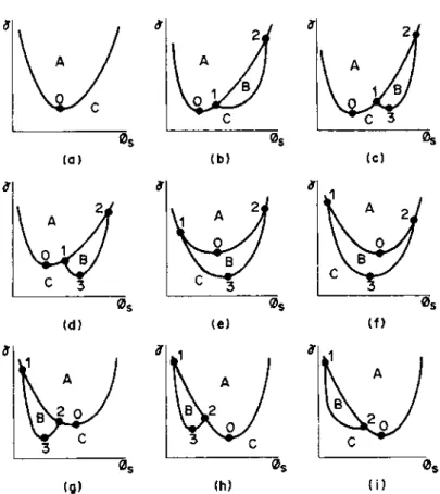
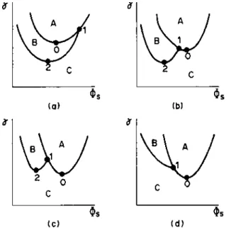
value of to, o = iQ. Neutral stability points are sketched in Fig. 1 for fixed values of

A and ,.

The upper curve in the sketches of Fig. 1 is given by (3.2), and it does not depend

on A. The function (3.2) has a unique minimum, yo, which is reached at Os =0,0

where 040 is the unique solution of

cosh 45(sinh2 4, + 242) + Os sinh fr

sinh 45(cosh2 Os- 244) + 3 0 cosh

'f

2 2

A A A

Os Os Os

(a) (b) (c)

A

0Os 0s

(d) (e) (f)

I~~~~~~~~~~ _{A AA}

Os Os 0s

(g) (h) (i)

The following equations are obtained from the real and imaginary parts of the

equation that results when (3.1) is multiplied by w+Okr and w is replaced by ifl

f= (AA _{_Q2) (A + 2 k. tanh Oj)2(cosh a + cos b)} -

(3.3) '~~~~'= Aj2Ok(b sinh a +asin b)

AA + 42_ _{80'(a sinh a - b sin b) - (a2+ b2)2(cosh a + cos b) tanh}

f,

(3Q4) 12 _ AwS 8QsIO(b sinh a + a sin b)

where a > 0 and b ?- 0 are given by

a2=2( +?k+&2+ 04), b2 =2(_+Ak2 + 4).

For fl = 0, (3.3) leads to (3.2), and (3.4) yields

(3.5) A, =442 (2O.+sinh 20J)/(3 sinh 2 , -64. -4k2 tanh 'k4.

If AA <(AA)m = 8.889* , (3.5) has no positive solution and neither has (3.4). If

AM > (AA)mq (3.5) has two positive solutions, O, and 'k2; for O, < , < 462, (3.4) is

seen to define a nonnegative function

(3.6) fl = fl(AA, Os)

which is such that AAt, _Os1) = Q(A,I1 O2)=O, fl(AM, Os) > 0 for O<, I <s < .2Q

The lower curve in the sketches of Fig. 1, which does not exist if AM < (AM1)m, iS

given by (3.3) with fl as given by (3.6). The coordinates of points 1 and 2 are (0,,, Yv)

and _{( 2, 'Y2), where y, and} Y2 are given by (3.2) with 0, t, and 0, = _{6s2, respectively.}

Point 3 (when it exists) is the unique minimum of the function

k.

defined by (3.3) and (3.6); its coordinates must be computed numerically.

For a fixed value of A, as A increases, the upper curve of Fig. 1 remains constant,

4,y decreases, 0,2 increases, and any point of the lower curve moves down. The

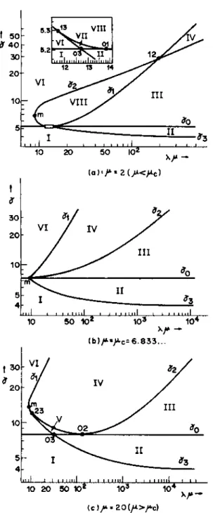
functions y, = y,(A9, Mu), _{for i = 0, 1, 2, and 3, are as plotted in Fig. 2, where y,/A,} -+

M/5, 9Y2/fXU-*2v3/A and Y3 -*4 as A -<X. The shape of the neutral stability curves,

y - _OS V is as one of the sketches of Fig. 1, depending on the relative position of points

0, 1, 2, and 3, which may be decided from the comparative values of A and A,.=

6.833 ... , and from the comparative values of AM and (AM)mg (AM)13,* , as indicated

in the caption of Fig. 1.

As is shown in Appendix A, for (4s, y) in regions A, B, and C of Fig. 1, the

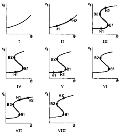
number of roots of (3.1) with positive real parts is one, two, and zero, respectively. Therefore, the steady state is unstable in regions A and B, and it is asymptotically stable in region C. Points of the upper curve correspond to bending points of the response curve, v, - k. At points of the lower curve, a pair of complex conjugate roots of (3.1), w = ? if, crosses the imaginary axis; at these points, a Hopf bifurcation occurs. Now, it is easily seen that the response curve is as in one of the sketches of Fig. 3,

depending on the region of Fig. 2 to which the point (AM, y) belongs. For example,

if M > Mc and (AM, _{y) e V the neutral stability curves, y - O,, may be as in one of the}

sketches (g) or (h) of Fig. 1; in such a sketch, the response curve corresponds to a

straight line y = _{constant, with max {yo, y3} < Y} < _{y2. Hence, the response curve is}

divided into five segments: O< ks < sHI; CsHI < Os < sH2; ksH2< s < ksBI; ksBI <

Ok3s < k.B2; and 'ksB2 < 0,1 in which the point (Os, y) belongs to regions C, B, C, A, and

C, respectively. Therefore, the response curve is as in sketch V of Fig. 3, with two bending points, BI and B2, and two Hopf bifurcations points, HI and H2. In Fig. 3,

no distinction is made in connection with the comparative values of kBI, kB2, 4kH1,

and kH2; for example, in sketch V, three additional possibilities could be considered,

862 1. E. PARRA AND J. M. VEGA

t50- . TVl

t40t

~

20 /

10 V,II

5 t3

10 20 5o 102 _{X,_}

{a) %jA2 (A<UC)

t

VI IV

20

10 ao

s A3

l ff 1 0 a I I 1 . , I , , ,*IIIf l 10 50 102 103 104

(b)PL11Ac= 6.8 33...

t 30 VIVI

t23 / III

10 02 to

0

II

5o- I3

4

,1 *, I ,.,, , I ,.,.,,,1 ,, 111I1 ,, 10 20 50 103 10

(C ) 2$: 20 (/4>jC)

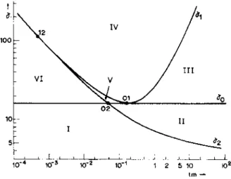
FIG. 2. Linear stability of Model 1 (slab geometry) for a fixed value of ,u. For iA < A, (respectively,

> ,a,), diagrams are qualitatively similar to diagram (a) (respectively, diagram (c)).

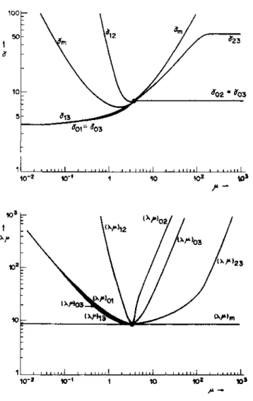
In order to get information about the size of the eight regions of Fig. 2, the coordinate of their vertices, as functions of ,u, are plotted in Fig. 4; observe that all

vertices come together as , -* uc, and that region VIII disappears as ,u -e Fc from below.

3.2. Arbitrary shapes of the catalyst. We consider Model 1 and a bounded domain, fl c RP (p = 2 or 3), whose boundary, dQ, is smooth and satisfies uniformly the interior

VS V5 VS

H2

82

HI

~~~~HI

0 0 0

I II III

VS VS VS

82 _B2 82

BI 81 BI

HI HI H2

0 0 0

rv V VI

VS VS H2

H2

82 82i

8B1 8,^1

0 0

VII VIII

FIG. 3. Response curves for Model 1 (slab geometry) and for Model 2. Asymptotically stable steady states. fH Unstable steady states.

for every point q of dfl, two hyperspheres, S1 and S2, of radius Pi and P2, are tangent

to dlQ at q, SI is included in Ql, and S2 and

nl

The steady state solutions of (1.3), (1.4) are given by

(3.7) AU,= 02U, inQl, u=1 ondQI,

(3.8)

Vs = I +/1 4 us dx = 1 +V1 lJ( d

)

ds,

in the terms of the parameter Os, where

(3.9) c2=ck2 _{exp (y/vs - y).}

Equation (3.7) uniquely defines a function Us = u,(Os, x), which is continuously

differentiable in its dependence on

_4,

k,

(3.10) _0<us(Os,x)<I forallxeCl,

(3.11) dn <s+(P -1)/P2 forallxeafl.

an

864 I. E. PARRA AND J. M. VEGA

100-

5 - a13

10-2 '01 1 1Q 10

jQ3

~ ~ ~ ~

(1)~02

'I (V"1. )03

102- (X')23

1 '' l'' i'. I I l t l i l l I I I 1 1 1 Ii I tti

10-2 101- 1 10 j0 o2 1

FIG. 4. Coordinates of the vertices of the regions of Fig. 2.

For fixed values of y and ut, (3.8), (3.9) define a C' response curve, OS (vs, 4).

The derivatives dvsld/d and dq5/dcAs are

(3.13) dvs 2g(vs - ds_, _Os + ₀₂ Ju dx dsa

'uL do

=s

a_adan

(3.14) 2/7' d = 2/ O - Yv-2 dS

where u = _ausl/a5 is the unique solution of

(3.15) sa-4 u = 245u, in f, ui= O on afl,

and satisfies, for all 4, > 0 (see Appendix B),

(3.16) ii(x) < O for all x e _Q,

(3.17) a >2p4s/e[p+(2p+1)p4s] forallxeafl,

The following properties are easily obtained (3.13)-(3.17):

(i) dvl/do, >0 for all 4, >0.

(ii) dl/do,>0ifOsk>0and

(3.18) Y(U -1 )/ v'sc1

(iii) If dl/d4s > 0, then

(3.19) y/ V2< ,ue[p +(2p + 1 )POAS/PSQ(o 2

The linearized problem around the steady state has nontrivial solutions of the

form u - us = X(x) exp (cut), v - vs = Y exp (cot), with Re cl) ' 0 only if (Y$ 0 and)

Z

= X/

(3.20) AZs(+ )Z = yV-202U in Q, Z =0 on adl,

(3.21) c/A +, = | Zdx+w(vs-)/v2.

In Appendix B, it is shown that:

(iv) If (3.20), (3.21) has a nonreal eigenvalue such that Re c _0, or if it has a

double real eigenvalue cv> _{0, then the following inequality must be satisfied:}

(3.22) ( //V2)[?/A + ,u- _u (V (- _ 1)/ V2] + 2+ k)3/A 2O4

where

(3.23) k = _(wpl/ V)2/P _{and cp = 2irxP/lpF(p/2).}

For given values of y, ,u and 45, and real values of w ' 0, (3.20) uniquely defines

a function Z = Z(c, x), which is continuously differentiable in its dependence on cv

and satisfies (see Appendix B)

(3.24) Z<0, -_0 for all v 0 and all x E 1,

&cv

(3.25) J

Z(w

Then, (3.21) may be written as

(3.26) co/A +,u = F(w),

where the function cl -e F(cw) is continuously differentiable and satisfies

(3.27) F'(cw))'0 forall cv?0, F(co)- yF(v - 1)/v2 as cv o-.

Furthermore, (2vs/y )Z(0, x) =&usl/&s (since it satisfies (3.15)), and

(go,) do

F(O) it-(s) d4,9

as comes out from (3.13), (3.14), (3.21). Then:

(v) Equation (3.26) has (at least) a positive real root if the inequality (3.18) is not satisfied and A is sufficiently large (because then , < F(co) for c sufficiently large). (vi) Equation (3.26) has no real positive roots if inequality (3.18) is satisfied

(because then j > F(co) for all Cv _{_ 0).}

866 1. E. PARRA AND J. M. VEGA

(viii) Equation (3.26) has no positive real roots if _d4l/do., >0 and A does not

satisfy (3.22). To prove this property observe that, since dl/do, > 0, the first member of (3.26) is larger than the second member for w = 0. If A = A1 does not satisfy (3.22),

then (3.22) does not hold for any A < AI. If, for A = A1, (3.26) had a positive real root,

then for some A = _A2 k 1, (3.26) would have a positive double real root (recall that F

is bounded); but this is not possible since A = _{A2 does not satisfy (3.22) (property (iv)).}

Now, from properties (i)-(viii) above, the following conclusions follow:

(A) The response curve, v,

- ),

than one S possibly), as it comes out from property (i).

(B) If y c 4 then (3.18) holds for all v, = 1 (i.e., for all 4)-0), and the response curve is monotonous (property (ii)).

(C) If y >4, let v,1 and v,2 be the solutions ofthe quadratic equation y(-v -1)! v2 =

1, let Os, and Os2 be the corresponding values of OSI, and let points 1 and 2 be the

corresponding points of the response curve. For 0 <

4)

(3.18) holds and dl/d4,>0 (property (ii)); then, if the response curve is not

monotonous, points 1 and 2 belong to the lower and upper branches of the response

curve; furthermore, the segments 0 < 4, < OsI and O)s2 < O)s correspond to asymptotically

stable steady states (properties (iv) and (vi)). On the other hand, in the segment

4)sI < 4?s < ,s2, inequality (3.18) is not satisfied (and the corresponding steady states

are unstable) if A is sufficiently large (property (v)).

(D) Finally, from properties (iii), (iv), (vii), and (viii), it comes out that if inequalities (3.19) and (3.22) are not satisfied simultaneously for any positive value

of Os, then a steady state is asymptotically stable or unstable according to whether

d4/ dos > 0 or d4/ dos < 0 at the corresponding point of the response curve. This simple

geometrical criterion applies, in particular, if one of the followiing inequalities is satisfied:

y _ 2+ 2V11 + 16k/A2 Vn,

A'aP2 + [P2A2 0 2

_________ 2__

AP2Sk+[P2/3+(p-1)Sj] k[H2(H,+2H2+1Hj+4H1H2-4) -27],

-4A2y3Op2V

A, <2kpSnj Vne[II/k p(2p+1)+1p2+ k2(2p+ 1)2],

where

HI = eA,VQP/kpSSQ, H2 =-Jkp(2p + 1)/p,

as may be seen when using (3.12).

4. Linear stability for Model 2. The steady state solutions of (1.6)-(1.8) are

Us =exp (Pse)/(1 + D), v = _{[m+(1+ m)4I/m(1} +,Ds)

in terms of the parameter 1,, which is given by

&2 =4os2 exp (y/vs - y).

The linearized problem around the steady state has nontrivial solutions if and only if

(4.1) (w+lm)- y2m2?5(1+41,) sw-4)2+ I I2+s,)

2[m + (1 + _m)1j,]2

for w $ 0 and w =0, respectively. Neutral stability points are as sketched in Fig. 5, where the upper curve is given by (4.2). The coordinates of point 0 are

4'o = m/(m + 1), y0 = 8(m + 1).

When w is replaced by ifl in (4.1), the following equations result

( a[m + (1 + _{M)4),]2[2lm(24)2+ a) + a(l} + a)(4)2S - a2)]

21m2)5(1 +4)5)(a - 24')

(4.4) f(2('+ a)+ Imb(a +1) 4S(2(D4s -a) - Qb(a + )

(4.4) Qikb(a + 1) - lm(24?)2+ a) fQa -)2b

where a > 0 and b _0 are given by

a =(D 2 + Jfl2 + 4)4), b2 =2( _ 2 + 4f)2 + .D4) +f

For 0<(s '- s,, (4.4) defines a nonnegative function

(4.5) Q = Q(lm, Os)

which is such that 51(lm,4(5s)=0, fk(Im, 0s)>0 for OK<(s<1s, where Ds, is the

unique solution of the equation

(4.6) Im = 4cF2(1 + 4s)/[1 + Ds + 2(1 +24)s)2].

The lower curve in the sketches of Fig. 5 is given by (4.3), with fQ as given by

(4.5). The coordinates of point 1 are (Dsl, y,), where y, is given by (4.2), with (Ds = (s,.

Point 2 (when it exists) is the unique minimum of the curve; its coordinates must be computed numerically.

As in Appendix A, the argument principle shows that in regions A, B, and C of Fig. 5, the number of roots of (4.1) with positive real parts is one, two, and zero, respectively. Then, the steady state is unstable in regions A and B, and it is asymptoti- cally stable in region C. Points of the upper curve of Fig. 5 are bending points of the response curve, and points of the lower curve are Hopf bifurcation points.

a'

a'

A A

1B 1

CC

Os Os

(a) (b)

B A B A

2 ₀

C C

Os Os

(c) (d)

868 1. E. PARRA AND J. M. VEGA

IV 12

100 \

III

VI V

~~~01

~

~

~

02

10 - I\ II

5

1 , , I , .

0o-4 103 10-2 10-1 1 2 5 10 102 lm-

FIG. 6. Linear stability of Model 2 for m = 1.

.~1 =11

10-4- /

io-5/

.1

~

103 -

10~~~~~~~~ -

102. 7.Coordintes ofthe verices ofthe reions ofFig. 6

For a fixed value of m, as I increases, the upper curve of Fig. 5 remains constant,

Isl increases, and any point of the lower curve moves down. For a fixed value of m,

the functions yi = yi(lm), for i = 0, 1, and 2, are qualitatively similar to those plotted

in Fig. 6. The asymptotic behavior of yi and Y2 is given by: Vhmy, -> 4m/N/3 as Im -+ 0,

y,/lm-*4(1+m)2/m as lm-coo; Y2-4 if m -1, y2 -(1+m)2/m if m>1, as lm .

The coordinates of the vertices of the six regions of Fig. 6 are plotted, versus m, in Fig. 7.

As in ? 2, the response curve is as in one of the sketches I-VI of Fig. 3, depending on the region of Fig. 6 to which the point (Im, y) belongs.

4.1. The limit m-O. In the distinguished limit Iy-m2-f-lm- 0, Yo=8 is

constant to leading order. The function (4.5) is given, in first approximation, by

f( D2(2+q)1I I2 'I

2

_4(2_+__)

. ~~Im (1 + 7)(4-2 q2- 773)' Im 2(1 + _7)(4-2772- _rq3)9

in terms of the parameter 71, for 0O -" _ 1, where

71 2= 2? / ((D2S +. fI2 + (D4),

and (4.3) may be written, in first approximation, in the form

4(m + FS)2 1+,(2 -q 2)

(4.8) =+22l2, mii

m V-- 7 24 + 2q +14 - 2772 _ 773'

Then, to leading order, yi is given by

yl = 4(v/i1/v'3 m) (ml/Jim+ v3/2)2,

and y3 is given by (4.8), with (D as in (4.7) and m/Jim as given by

m (Ds 4773(2+ 7j)(1 + J)(6- -72)

N'T1_i VT'1_ 3,7 12776+27,5-56Y4 - 92 77- 16772+88iq +64f

A plot of the linear stability diagrams of Fig. 6 in this limit is given in Fig. 8,

where (lm)O/m2=4/3, (lm)02/m2=0.3138* * , _{(lm)12/m2=4/1875, YO1= Y02=8, and}

Y12 2 .262/25.

100-

12 XIV

5 1

1 VI | I , , I I, ,

VI~~~

10 0

02

10-2 10 1 2 5 _{10 M.m} jo2

870 1. E. PARRA AND J. M. VEGA

4.2. The limit m - _{oo. In the distinguished} limit D2 _ _m i _{1, m} -+ _{oo, (4.2) and}

(4.3) may be written, in first approximation, as

(4.9) yl m = 2(I + (D,)2/,D"

(4.10) y/m = _{a(1 +cj)[21m(2D2t+ a)+ a(l} + a)(4?2- a2)]/21m4>s(a2-242).

Therefore, to leading order, yo/ m = 8 and y1/ m is given by (4.9), with IS, = 4s,,, where

(L is the unique root of (4.6). y2/m must be computed numerically, as the unique

minimum of the function 4 e- y/m, defined by (4.5) and (4.10). A plot of the linear

stability diagram of Fig. 6 in this limit is given in Fig. 9, where (Im)12 = 0.001860O >

(lm)02 = 0.1430 _{* , (tm)O1} = _{0.4, Y21/m} = _{55.63**, and y02/m} = _{>y1/m =} 8.

5. Hopf bifurcation. Let us now consider local Hopf bifurcation at points HI and

H2 of Fig. 3. For the sake of brevity, only Model 2 will be considered; a similar analysis applies to Model 1.

1 2

t s _IV /

VI

10- 0

0

5 II

1 _1;ttt

.1,l...1tI I

io-3 V2 IoT 1 2 5 10 102 lm-

FIG. 9. Linear stability of Model 2 in the limit m e oo.

Let a be a parameter (to be chosen later) giving a first approximation of the size

of the bifurcated periodic orbits, and let 4H be 'DIHy or CH2. When using O. as

bifurcation parameter, it is expanded in the form

Ps =4)H+Ba2+**

Then, if (sH -)sHl (respectively, )sH = 4)sH2), the bifurcation is subcritical or super-

critical depending on whether B <0 or B> 0 (respectively, B> 0 or B < 0).

In order to simplify the algebra of the analysis below, we shall use y as bifurcation

parameter. To this end, y will be expanded as

(5.1) y= y+Aa2+a.

If the lower curve of Fig. 5 is given by y =f(Qs) (then y, -f(ISH)),f(f .?H) is negative

or positive depending on whether (tH = (sHI or 4 H )S H2 It is easily seen also that

B =-A/f((Ds H). Therefore, bifurcation at 4P?H is subcritical if A <0, and it is super-

For 0< (DsH < (sH1 ,the pair of roots of (4.1) that (for varying y and fixed F. _{= 4,H,}

1, and m) crosses the imaginary axis of the complex plane at y = _{y, satisfies the}

transversality condition

d(Re w)/dy 0, Im w = f, ?0,

at y = y,, while the remaining roots of (4.1) have strictly negative real parts. In addition, the solution of (1.6)-(1.8) satisfies the smoothness hypothesis of Hopf bifurcation theorem (Marsden and McCracken [9], Hassard et al. [10]), as is seen by means of standard theory on semilinear parabolic equations (see, e.g., Hassard et al. [10], Henry

[11]). Hence, the Hopf bifurcation theorem shows that, for y sufficiently close to yc

(i.e., for y as given by (5.1) and a sufficiently small), there exists a periodic solution of (1.6)-(1.8), of period

(5.2) T(a) = 27T/fl with flQfl + af, + aa2Q2+ *

which may be written in the form

(5.3) U= U,+aUo+a2Ul+a3U2+ *, _{v=v,+ av,+a2v2+} .

Furthermore, bifurcated orbits are unstable if bifurcation is subcritical (A<0), and they are orbitally, asymptotically stable if bifurcation is supercritical (A> 0).

The coefficients of the expansions (5.1)-(5.3) may be calculated systematically by means of known recursive formulae (Hassard et al. [10], Kielh6fer [12]), via reduction to the center manifold, that also allows us to analyze degenerate cases in which the transversality condition is not satisfied. Nevertheless, due to the inherent algebraic complexity of the problem (1.6)-(1.8), we shall use a more direct (although a less systematic) approach, and we shall not try to analyze degenerate cases in detail. Some conclusions about the nature of degenerate cases may be drawn from the results for neighboring nondegenerate ones, by means of simple normal forms arguments (Golubitsky and Langford [13], Guckenheimer [14]), when taking into account that the flow defined by (1.6)-(1.8) is essentially two-dimensional near a bifurcation point, since it may be reduced (locally) to a center manifold for sufficiently large time.

In order to look for 2iX-periodic solutions, we introduce the new time variable s = 2ifr/ T, where the period T is given by (5.2). Then, A, fki, Ui, and vi, the coefficients of the expansions (5.1)-(5.3), may be calculated from the set of recursive problems which results when the expansions (5.1)-(5.3) are inserted into (1.6)-(1.8), and the coefficient of each power of a is set to zero. Such problems are of the form

(5.4) fc

_as

(5.5) UQ=0 ate=-oo, a ui +U,=O at 4=0,

(5.6)

Qc d

_{df =}

where fo 0 and gO 0. In addition, we impose the periodicity conditions

(5.7) Ui(0, g) Ui(2ir, (), vi(0)= vi=(2r),

and an additional condition in order to define the parameter a; this condition, which

is quite arbitrary, may be, for example, v(0) = _{vs + 2av 2/ Yc, v'(0)} = _{0, or vo(O)} = 2v2/ yC,

872 1. E. PARRA AND J. M. VEGA

It is easily seen that (5.4)-(5.6) has a solution satisfying (5.7) only if the second members of (5.4) and (5.6) satisfy the solvability condition

(5.8) { exp

(-is)(

o -00,

where

X = 1D_H Y*(1 -exp (v/'HD+ QC ()/(1 +'/?sH + ilC))/()2H + ifQ), Y'* 0

is a nontrivial solution of the adjoint linearized problem:

de2 (SsH + iQS)X+ H Y* = _{? in-ax <}

e

0,

X*boundedat =-oo, dX*+X*=O atS=O,

ro

~

~ ~

ycVs2sHD USX* _{d6+incY*+1m[I-} y (v, - 1)/vV] y* 0.

_00

When UO and vo are inserted into the second terms of (5.4) and (5.6), it is easily seen that the solvability condition (5.8) is satisfied for i - 1 only if Ql =0. Then U1 and v1 are easily calculated; when they are inserted into the second members of (5.4) and (5.6), and the solvability condition for i = 2 is applied, a pair of linear equations is obtained to calculate f2 and A. The solution of these equations yields

(5.9) A = y[ C1 (1 + C3) + DI 1D3]/[Im( 1 + C3) + fD3],

where

C-?s2 ( + El ) - El - 2 C2 -2E4] + E2 + E3( C2 + El ) + 2Ql(1 - E4),

DI =PD2[D3(1 +E,)-2D2 +(2(p2 - E3)/2fl]

+fl[2(E4- 1)(C2+ E,) -2E4+3E 2] + D2E3,

C2 =(C4C5- D4D5)/( C5+ D), D2 =(C4D5 + CD4)/(C5+ D)

C3+ iD3 =l4D3(D6- iC6)(1 + C8+ iD8)/y(1 + :1) E2

C4 = f12[CP. + 2 ym (1 + F)Ej(E4- 1 )] + dI (C7 - _{2 C8) -JD7/2}

D4= 2y(I + Fs)Y3E2(2E4- 1)/ I + 15s( _{D7 -22D8) + 43,fIC7/2,}

C5= 2f2['Fs

-

+

D5-

+

(D

C6+iD6= 1+2vsI?5+iQ _______________

((I)p2 + in)( I + J/)2 + in) (1),( I + Is )((I) s + 8/I?2+

C7+ iD7 = _(D,(1 + (Ds)/(1 + J(p2+2i)j4 2+2if-1,

C8+ iD8 = _{Po(D +FS)/(1+Js} + r

in?

+

4ym(1 +cP)2E2(E4- 1)+(),(3+44Ps)+4(1 +(s)C8/ 02

1 _-

1)s -2ym(1 + ps _)2E2

E2= Im(1 -3E4+3E4), E3 = Im(2E4-3)+2143/y(I +1)()E4

E4= [m +(1 + m)4js]/ym(1 +Is).

Here, the suffixes H and c have been dropped from 4(D, fl, and y; also y and Ql are

given by (4.3) and (4.5). Therefore, (5.9) defines, for 0<-?s < F , a function of the

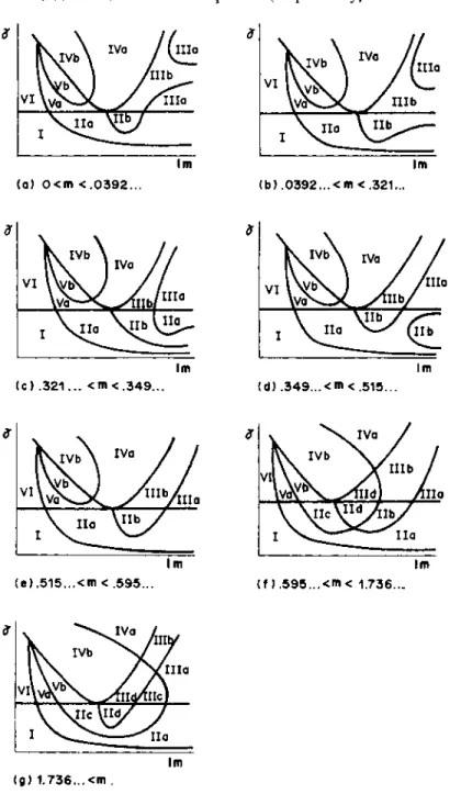
HI and H2) is subcritical or supercritical. Numerical computations are summarized in Figs. 10 and 11; in the regions IIa, * * *, Vb (respectively, I and VI) of the diagrams sketched in Fig. 10, the response curves are as sketched in Fig. 11 (respectively, in Fig. 3). Observe that the diagrams of Fig. 10 are partitions of the diagram of Fig. 6. The dynamic response of the catalyst in a quasi-steady operation (i.e., when the parameters are varied slowly enough) near a point of neutral stability, depends on whether Hopf bifurcation is sub- or supercritical at this point. In the supercritical (respectively, subcritical) case, as the steady state becomes unstable, neighboring initial conditions lead to oscillations of small amplitude (respectively, to some other attractor,

ivb Iva III(. Iva

VI IIIIVI V

Im Im

Im Im

Im Im

(c) .321... <m<349.. .349.<m<.5T5... (d)

if~~~~FG .Hp bfraionforMdl2

VI ~~~~~~~~VI\~IIIb/

Im I1m

(e).51 ... m < .95...(fY. 5 95... < m< 1.7 36...

a'~

~ ~

v

I

Im Cg) 1.736... < m

874 1. E. PARRA AND J. M. VEGA

VS Vs Vs

0

0 0

.0 00~~~~~~~~

00 .0~~0

0~~~~

Ila IIb IIc

00~~~~~~~~~~

IIIc IIIQ IIVa

IVb V a V b

0% 0~~~~0

00 0 0

lIII IIId Ivab

VS VS VS

~~~00

~~~~0 0

o

IVb Va Vb

FIG. 1l. Response curves for Model 2. Asymptotically stable steady states. +1-fI-I-f Unstable steady states. a00-0 Orbitally asymptotically stable periodic orbits. 00000 Unstable periodic orbits.

far away from the steady state), and the transition through the instability limit is (respectively, is not) smooth, as far as the dynamic response of the catalyst is concerned; therefore, such a response depends qualitatively on the shape of the actual response curve, which is as one of those sketched in Fig. 11 if it exhibits Hopf bifurcation phenomena.

The analysis of the degenerate bifurcations that take place on the lines and vertices of the diagrams of Fig. 10 is beyond the scope of this paper. Such an analysis would provide predictions about the global shape of the bifurcated branches of periodic orbits. The following degeneracies are present in the diagrams of Fig. 10:

(a) On the common boundary of the regions VI and Va, and of the regions I and Ila, two Hopf bifurcation points coalesce; since both bifurcations are supercritical near this line (see sketches hIa and Va of Fig. 11), both branches are connected near the transition, and coalesce as the line is approached from above.

The (two-dimensional) universal unfolding of this (codimension two) degeneracy

contains Hopf bifurcations and saddle loops as mechanisms leading to periodic orbits

(see [14]); therefore, saddle loops are expected to occur near this line.

(c) On the upper boundary of regions I and II (= Ia u lIb u IIc u IId), a (static)

bifurcation takes place, associated with a cusp singularity.

(d) On the points of intersection of the three above-mentioned lines, a degenerate

bifurcation of higher codimension takes place.

(e) On the remaining lines of the diagram, a higher-order Hopf bifurcation takes

place, whose analysis requires us to calculate two more terms in the expansions

(5.1)-(5.3) and provides the transition from subcritical to supercritical Hopf bifurcation

(see [13]).

6. The case af = 0(1). In the limit

L -c _o, ,l3 o*0, pI> _{Oil a=O(l)}

two isothermal models are obtained from (1.1), (1.2) by means of an analysis which is similar to that in ? 2.

If 02 exp (y- y/vj) = 0(1) (v, is any steady state temperature of (1.1), (1.2)), then

one obtains the model (1.1), (1.4). A linear stability analysis of this model leads to qualitatively similar results to those in ? 3.

If 42 exp (y - y/vj) is large (i.e., 52 >> 1 if y = 0(1)), then the following model is

obtained

aW a2W

(6.1) _{dT a T} g2 _2w exp (y -y/v) _{in -oo < ;< ,}

(6.2) w=O atg=-oo, _{-w =1 atCg=O,}

(6.3) dv =Am(1-v)+Aexp(y-y/v) 4 wdg,

with

A= ,3LSQ/)2 V0, _{m = V/'0,} T = 42t, _{C= 77.}

Here, 77 is a coordinate along the outward unit normal to al, and w is the mean value

of 4u/oa at time T over the surface g = constant. Observe that (6.1)-(6.3) differ from

the model (1.6)-(1.8) only in the boundary condition at g = 0. The new boundary

condition makes it possible to reduce the analysis of the global dynamic behavior of

(6.1)-(6.3) to the following two-dimensional dynamical system:

dW

(6.4) d- = 1- Wexp (y-y/v),

dT

(6.5) dv = Am(1 - v) + A W exp (y - y/ v),

where W = _{w dC ((6.4) is obtained upon integration of (6.1) and substitution of}

the boundary condition (6.2)).

The model (6.4), (6.5) may be obtained also from the equations of a continuous stirred tank reactor without cooling (see, e.g., [6]) in the limit of large Damkohler and Lewis numbers. Also, model (6.1)-(6.3) (and, hence, model (6.4), (6.5)) may be

876 1. E. PARRA AND J M. VEGA

y = 0(1)); a simple singular perturbation analysis shows that, after an initial time

stage, U(f, r) and v(zr) are given by (6.1)-(6.3), with

A =l1/D2, (De, T=P2T, W= FU.

Model (6.4), (6.5) has a unique steady state,

W=exp[-y/(m+1)], v=1+1/m,

that is linearly asymptotically stable if y _ (m +1)2/ or if y> (m +1)2/rm and

Am[ym/(m + 1)2_ 1] < exp [y/(m + 1)],

while it is unstable otherwise. At neutral stability points, there is a Hopf bifurcation,

which is subcritical if m < 9 - 26? 0.515 and max { y-, y*} < y < _{y+, where}

Yf = (m + 1)[m + 3 _{?Jm2_} 18m +9]/2m, ye - (m + 1)2/ m,

while it is supercritical if 2 < m < _{9 - \2 and} ye < y < y_, or if 0 < m _9 - 2V6 and

y > y+, or if m > 9 - 2v'6 and y > y*, as is easily seen. These results do match with

those obtained in ? 6 for D2 = _{p2 exp (y-y/ v,) - l- oo.}

It is easily seen also that as A-> cx, the system (6.4), (6.5) exhibits relaxation

oscillations provided that y> y>, (i.e., provided that its unique steady state is unstable

as A--oo).

7. Concluding remarks. Two isothermal models have been derived from the non- isothermal model (1. 1), (1.2). They are appropriate for the analysis of nonlinear stability

of the steady states of (1. 1), (1.2) under small perturbations in the limit y, -> 0, v - 0,

L -->X, oa -> c. If, in addition, y = _{0(1), then they are also valid in studying global}

stability properties.

The linearized stability of the steady states for Models 1 and 2, and local Hopf

bifurcation for Model 2, have been considered in ?? 3-5. Some remarks about the

results are in order:

(a) For a fixed value of g, the linear stability diagram of Model 1 for the slab geometry is as one of those in Fig. 2. Oscillatory instabilities appear in a region of the

response curve if and only if A,t > 8.889 and yl/ < y < Yc2, where _Yc,

min { y1, Y2, 73} and Yc2 =max {y1, Y2}-

(b) For arbitrary shapes of the catalyst in two and three dimensions, it has been shown in ? 3.2 that oscillatory instabilities do not appear if A, is sufficiently small or if y is sufficiently small or large (for fixed values of A and A), while they do appear

in a region of the response curve if y > 4 and A is sufficiently large (for fixed values

of y and p). This result makes it reasonable to conjecture that for arbitrary shapes of the catalyst, linear stability diagrams are qualitatively similar to those obtained in ? 3.1 for the slab geometry.

(c) For a fixed value of m, the linear stability diagram of Model 2 is as that in

Fig. 6, which is plotted in Figs. 8 and 9 in the limits m -* 0 and m -> oo, respectively.

Oscillatory instabilities appear in a region of the response curve if and only if y > y, -

min {yi, Y2}.

(d) It has been shown for lumped chemically reacting systems and conjectured for distributed systems (Ray and Hastings [6]) that a given steady state of the lower or upper segments of the response curve is stable or unstable according to whether the Lewis number is smaller or larger than some bifurcation value (that can be infinite). This conjecture is true for Model 1 in the slab geometry and for Model 2. In fact, for

Model 1 for example, the instability bounds, 4sHI and PsH2, are such that O'sHI decreases

and 0,H2 increases as A increases (for fixed values of y and tL), as seen from the

(e) In the limit lI-ao, m = 0(1), it is easily seen that the lower curve of Fig. 5

has two distinguished parts. For 4), - _{1, it is given by}

y = _{[m + (m + 1)4)?]2/Mr4)S(1} + )()

in first approximation, while for 1 << _{4), < ),I = 2ml + 0(1), it is given by}

y=(m+1)2/m+(m+1)2)2/n2l

Hence, if m<1 and 4<y<(m+1)2/m, then

4)sH2- [y-2(m + 1)+y(y-4)]/2[(m+ 1)2/m -y] as l-c,

while 4)sH2+o as lcx if y?(m+l)2/m (if m '1 and 4 <y< (m+l)2/m, then every

steady state is linearly stable and the point H2 does not exist). Therefore, there exists

a critical value of the activation energy, yy* = (m + 1)2/rm, such that if y '- y* then the

upper instability bound, OH2, iS such that OH2 -ooX as l-* oo (for fixed values of y and

mi). The same type of behavior is found for the isothermal model (1. 1), (1.4) in arbitrary domains, for finite values of a and for more general kinetic laws (see [4]).

(f) In the limit 4) -e ox, Model 2 is reduced globally to a two-dimensional dynamical

system that exhibits relaxation oscillations as 1/4)2 _ CX if y> y* = (M + 1)2/m, as was

shown in ? 6. We may ask whether Models 1 and 2: (i) possess a two-dimensional

global attractor, and (ii) exhibit relaxation oscillations as A - 0x or 1 - x whenever

every steady state becomes unstable in that limit. Although it may be proved that Models 1 and 2 possess a finite-dimensional global attractor by using results for more general reaction-diffusion problems, finding precise bounds on the dimension of the attractor is not an easy task (see [15] and references given therein). It seems that the answer to the second question requires an involved multiple time scales analysis that would be much facilitated if an answer to the first question were available.

The above-mentioned dynamical system is obtained also for o- = 0(1) if k2 iS

sufficiently large, as was seen in ? 6. This system is a submodel of the widely used model of continuous stirred tank reactor without cooling, but differs quantitatively from the system that one would obtain by means of lumping procedures (see, e.g., [1]), as could be expected.

Appendix A. Let 1i be an analytic function inside and on a closed contour F of

the complex plane, without zeros on F. The argument principle (see e.g. Ahlfors [16])

provides the number of zeros of i _{inside F, as N = AI arg 1/2} IT, where Al arg

/

change in value of the argument of 1/ _{when F is transversed once in the positive sense.}

In order to calculate the number of roots of (3.1) in the right-hand side of the complex plane, we write (3.1) in the form

(A.1) *(c) Hw2+ + K [(tanh + q5)/ k, - (tanhJw+dX)/1w+1 ] =0

where

(A.2) H = Ayt - K(tanh k3/j/3, K = 2Ayt2 y4/(F( +20, tanh 0k)2,

and consider a contour F consisting of four segments: r,: a = R exp (i@), for _-7T/2 <

0 < 7T/2; [2: w = ifl, for R _{' Ql-' r; F3:w = r exp (i@), for !/2} > O _{> -T/2; and} F4: w =

ifl for -r ' fl-Q'-R. Any root of

fr

small and R is sufficiently large.

From the asymptotic behavior of 1i _{as lwI-)-0 and as}

Iw

(A.3) Al, arg 4i=2IT+E1, A1l- arg 1 = -IT+E3,

878 I. E. PARRA AND J. M. VEGA

In order to calculate A arg qi on r2 and r4, let us consider the functions fl -) _{J, (fl)}

Re qif(ifl) and fl-*J2(fl) = _{Im 4i(ifk), which are given by}

(A.4) J1(CQ) = _{-_f2+ K[(tanh ck)/ ), -2(a sinh a + b sin b)/(a2+ b2)(cosh a +cos b)],}

(A.5) J2(Qf)- Hfl+2K(b sinh a-a sin b)/(a2+b2)(cosh a +cos b),

where a+ib=2f 02+ifl, as in ?3.1.

Since J, is an even function of fl, and J2 is an odd function of fl, it is clear that

(A.6) Al-, arg li# = Al4 arg q'.

On the other hand, for a fixed value of 0,, the equations J, = 0 and J2 = 0 define

two functions,

K =fi(Q), H/K =f2(0),

respectively, which are easily calculated from (A.4), (A.5), and are seen to be

monotonously increasing. Furthermore, f1(O) = K, f2(0) - H//K., where

1645 cosh2

.

3 sinh 24, -64) _-442 tanh , Km 44 cosh2 4)

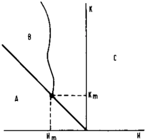
and fi -e 00, f2 -e 0 as fl -- ocx. Therefore, the curve H =f1(fl)f2(Q7), K =f1(f7), 0 < fl < ,

is as the upper curve of the sketch of Fig. 12, and consists of points (H, K) for which

(A.1) has a pair of purely imaginary roots, w = ?ifZ. For points of the lower curve of

Fig. 12, which is the straight line K/H = Km/ Hm, (A.1) has w = 0 as a double root.

Now, A arg e/ along F2 is easily calculated, for (H, K) in regions A, B, and C of Fig.

12, from the shape of the graph of the function fl -> _{F(Q) Im 4f(i1f1)/Re ef(iil)}

J2(fl)/J,(17), for 0 < < oo.

If (H, K) belongs to region A, two cases must be considered. If K _ K_, then

F >0 for 0 <fl< co, F - oor as fl-*0 and F -+0 as fl-+oo. If K > K., then JJ(l) = 0

for a certain Cl, such that 0 < fl < oo, F < 0 for 0 < f < fl, F > 0 for fl < f < o,

F-*-oo as fl -0 and as fl -W, F-*+cc as fl -* fl and F 0 as fl a. Therefore,

in both cases

(A.7) _{A1,,arg4'=vr/2+E2 for(H,K)eA,}

where E2 0 as R-o*o and r -0.

K

A K M

Hm H