University of Technology, Sydney
Faculty of Engineering and Information Technology
ARTIFICIAL INTELLIGENCE FOR CANCER
TREATMENT AND DIAGNOSIS
By
Juan Martinez de la Pedraja Garcia
Student Number: 12973525
Project Number: SU-031
Major: Mechatronic
Supervisor: Dr Paul Kennedy
A 6 Credit Point Project submitted in partial fulfilment of the requirement
for the Degree of Bachelor of Engineering
3
ABSTRACT
Currently, according to some estimates diagnostic errors contribute to approximately 10 percent of patient deaths, which explains the interest in incorporating new technologies into this process. With the significant developments made in the last decades, Artificial Intelligence (AI) has arguably become a good candidate for this task. Specifically, our project involves using Machine Learning (a subfield of AI) to improve childhood cancer treatment and diagnosis.
We will focus on Acute Lymphoblastic Leukemia (ALL), the most common type of pediatric cancer with around 300 yearly diagnoses in Australia. In ALL, relapse decreases the chances of survival as standard chemotherapy becomes ineffective. Thus, modified therapy is needed for patients with high risk of relapse. In this project, we explore the use of Machine Learning to accurately predict relapse, which would ultimately result in better treatment. This study will be based on a dataset containing genetic information, which will be the basis for predictions, and cancer outcome (relapse/mortality) of about 150 patients.
The low number of samples, combined with the high proportion of non-relapse cases, means there are very few relapse examples, which complicates finding meaningful patterns to make accurate predictions. Furthermore, high dimensionality creates difficulties when trying to achieve generalizable solutions. To address these challenges, we explore the use of biased classifiers, particularly sparse linear methods; dimensionality reduction techniques both supervised (univariate feature selection, LDA) and unsupervised (PCA, Autoencoders); ensemble approaches, especially bagging and undersampling/oversampling methods (ENN).
4
LIST OF CONTENTS
STATEMENT OF ORIGINALITY ... 2 ABSTRACT ... 3 LIST OF CONTENTS ... 4 LIST OF FIGURES ... 7 LIST OF TABLES ... 8 NOMENCLATURE ... 10 1. BACKGROUND ... 111.1 Introducing Machine Learning ... 11
1.2 The Importance of Better Medical Diagnosis and Treatment ... 11
1.3 Several Examples of Recent Research ... 12
2. PROJECT OVERVIEW ... 14
2.1 Scope and Objective ... 14
2.2 ALL and the Importance of Relapse... 14
3. METHODOLOGY ... 15
3.1 Machine Learning Methodology: An Empirical Iterative Process ... 15
3.2 A Framework for Machine Learning Methodology: The Bias-Variance Trade-Off ... 16
3.3 Ensuring Validity of Results ... 18
3.4 Evaluating Performance: Metrics ... 20
3.5 Resources ... 21
4. PRELIMINARY ANALYSIS AND DISCUSSION OF GENE EXPRESSION DATA ... 22
5
4.2 The Challenge of Low Number of Samples ... 22
4.3 The Challenge of Class Imbalance ... 23
4.4 The Challenge of High Dimensionality ... 25
4.5 Changing Perspective: A Quick Look from the Bias-Variance Viewpoint ... 26
5. EXPLORATORY PHASE ... 26
5.1 Brief Assessment of Several Model’s Performance ... 26
5.2 Brief Analysis of Results ... 32
5.3 Analysis of the Logistic Regression Model ... 33
5.4 Conclusion ... 38
6. DIMENSIONALITY REDUCTION ... 38
6.1 Establishing a Target Number of Dimensions ... 38
6.2 Supervised vs Unsupervised Dimensionality Reduction ... 38
6.3 Supervised Dimensionality Reduction ... 39
6.3.1 Decision Tree Based Methods: Feature Importance... 39
6.3.2 Linear Discriminant Analysis ... 39
6.3.3 F-test Based Feature Selection ... 40
6.4 Unsupervised Dimensionality Reduction ... 44
6.4.1 Dimensionality Reduction Based on Linear Dependency ... 44
6.4.2 Principal Component Analysis ... 48
6.4.3 Autoencoders ... 50
6.4.4 Manifold Learning ... 53
7. OTHER STRATEGIES FOR VARIANCE REDUCTION ... 54
7.1 Outlier Removal ... 54
6
8. RESULTS ... 56
8.1 Genes Selected by L1 Penalty ... 56
8.2 Baseline Model ... 56
8.3 Bagging, Feature Selection and Outlier Removal Combined... 59
9. CONCLUSION ... 59
7
LIST OF FIGURES
Figure 3.1: Bias-Variance Trade-Off, Overfitting and Underfitting (Halls-Moore 2015)
... 17
Figure 3.2: 4-Fold Cross Validation (Flöck 2016) ... 20
Figure 4.1: The Effect of Irrelevant Features on Distance Based Methods ... 24
Figure 5.1: Frequency of Selected Genes in 10-Fold Cross Validation ... 34
Figure 5.2: Correlation Matrix of Selected Genes in 10-Fold Cross Validation ... 35
Figure 5.3: Frequency of Selected Genes in 100 Iterations of 10-Fold Cross Validation ... 36
Figure 6.1: F-Statistics of All Genes in the Dataset ... 41
Figure 6.2: F-Statistics of the 2000 Most Relevant Genes ... 41
Figure 6.3: F-Statistics of the 500 Most Relevant Genes ... 42
Figure 6.4: Correlation Matrix of the 50 Most Relevant Genes According to the F-Test ... 43
Figure 6.5: An Example of a Plot of Cumulative Variance (Géron 2017) ... 49
Figure 6.6: Cumulative Variance of the Features ... 50
8
LIST OF TABLES
Table 5.1 Naïve Bayes Training and Validation Performance ... 29
Table 5.2 Support Vector Machines (No Class Weights, Sigmoid Kernel, Gamma=0.001, C=10) Training and Validation Performance ... 29
Table 5.3 Logistic Regression (Balanced Class Weights, L1 Penalty, C=0.1) Training and Validation Performance ... 30
Table 5.4 Stochastic Gradient Descent Classifier (Log Loss, Balanced Class Weights, L1_Ratio = 0.5, Alpha = 2) ... 30
Table 5.5 Decision Tree (Balanced Class Weights, Entropy Criterion, 0.2 Minimum Weighted Fraction at Leaf) ... 30
Table 5.6 Random Forests (Balanced Class Weights, Entropy Criterion, 0.2 Minimum Weighted Fraction at Leaf, 10 Estimators, 0.01 Number of Features, No Boostrapping) Training and Validation Performance. ... 31
Table 5.7 Extremely Randomized Trees (Balanced Class Weights, Gini Criterion, 0.1 Minimum Weighted Fraction at Leaf, 10 Estimators, 0.1 Number of Features, No Boostrapping) Training and Validation Performance. ... 31
Table 5.8 Adaboost (Balanced Class Weights, Entropy Criterion, 0.15 Minimum Weighted Fraction at Leaf, 10 Estimators, 1 Learning Rate) Training and Validation ... 31
Table 5.9 Baseline Model: Logistic Regression (Balanced Class Weights, L1 Penalty, C = 0.1). ... 33
Table 5.10 Baseline Model with L2 Penalty: Logistic Regression (Balanced Class Weights, L2 Penalty, C = 0.1). ... 33
Table 5.11 10 Most Frequently Selected Genes by the Baseline Model. ... 37
Table 5.12 Logistic Regression Model (Balanced Class Weights, L2 Penalty, C = 30) With 10 Selected Genes. ... 37
9
Table 6.2: Logistic Regression (Balanced Class Weights, L2 Penalty, C= 30) with 50 Genes Selected by ANOVA. ... 43
Table 6.3: 10 Most Relevant Genes According to ANOVA. ... 44
Table 6.4: Unregularized Logistic Regression (Balanced Class Weights, L2 Penalty, C = 1000) with PCA. ... 48
Table 6.5: Neural Network (Two Layers of 10 Neurons, 0.3 Dropout Rate and 0.4 L2 Regularization on Second Layer) ... 48
Table 7.1 Logistic Regression (Balanced Class Weights, L2 Penalty, C = 30) Combined with ANOVA Feature Selection and ENN Outlier Removal. ... 54
Table 7.2 Bagging Ensemble of Logistic Regression Models (Balanced Class Weights, L2 Penalty, C = 30) Combined with ANOVA Feature Selection and ENN Outlier Removal. ... 55
Table 8.1 Test Results of Logistic Regression Model (Balanced Class Weights, L2 Penalty, C=30) Based on 10 Genes Selected by L1 Penalty. ... 56
Table 8.2: Test Results of the Baseline Model (Logistic Regression with Balanced Class Weights, L1 Penalty and C=0.1). ... 57
Table 8.3: Comparison of Cross Validation and Test Results for Different Train/Test Splits. Logistic Regression with Default Parameters (L2 Penalty, C=1) and Balanced Class Weights. ... 58
Table 8.4 Bagging Ensemble of Logistic Regression Models (Balanced Class Weights, L2 Penalty, C = 30) Combined with ANOVA Feature Selection and ENN Outlier Removal. ... 59
10
NOMENCLATURE
ADASYN: Adaptive Synthetic Sampling
AI: Artificial Intelligence
ALL: Acute Lymphoblastic Leukemia
ANOVA: Analysis of Variance
AUC: Area Under the Curve
CNN: Convolutional Neural Network
FFNN: Feed Forward Neural Network
FN: False Negative
FP: False Positive
LDA: Linear Discriminant Analysis
PCA: Principal Component Analysis
SDAE: Stacked Denoising Autoencoder
SGD: Stochastic Gradient Descent
SMOTE: Synthetic Minority Oversampling Technique
SNP: Single Nucleotide Polymorphism
TP: True Positive
11
1. BACKGROUND
1.1 INTRODUCING MACHINE LEARNING
Artificial Intelligence (AI) is not as recent as it may seem as it dates back to the 50’s. However, with the exponential development of technology and its consequent increase in computational power, AI is becoming an increasingly central subject in our societies that is thought to lead to dramatic changes (Harari 2017). However, at this given point in time, we are still at an early stage of development where it is only feasible to attempt low level tasks, such as pattern recognition. This is precisely one of the foundations of Machine Learning, upon which this project is based.
Machine learning can be described in several forms, a common and broad definition states that it consists in making machines learn from data (Buduma 2017; Géron 2017). Traditional solving problem approaches were based on deduction: starting from one or more mathematical/logical principles, a set of precise programmable instructions that lead to a solution were derived. On the other hand, machine learning is based on induction: using given examples, a model that fits the data is proposed, hoping that it will generalise to future cases (Kirk 2015). This becomes especially useful for problems which we know are governed by an underlying pattern, but this cannot be effectively described mathematically or logically (Abu-Mostafa et al. 2012). Some examples are: image/speech recognition, fraud detection, product recommendation, online search, financial trading and some medical applications such as drug and vaccines discovery, epidemic outbreak prediction or medical treatment and diagnosis, the latter being the subject of this project, specifically applied to childhood cancer.
1.2 THE IMPORTANCE OF BETTER MEDICAL DIAGNOSIS AND TREATMENT
According to a report made by the Institute of Medicine from the National Academies of Science, Engineering and Medicine (2015, p.2): ‘diagnostic errors contribute to approximately 10 percent of patient deaths, and medical record reviews suggest that they account for 6 to 17 percent of adverse events in hospitals’. It is estimated that between 40 000 and 80 000 people die each year as a result of misdiagnosis and that 10% of all hospital deaths had a major diagnostic error (Winters et al. 2012). In the case of cancer, early diagnosis is critical and the best guarantee of survivability. For instance, according to Cancer Research UK (2015):
12
‘more than 90% of women diagnosed with breast cancer at the earliest stage survive their disease for at least 5 years compared to around 15% of women diagnosed with the most advanced stage of disease (…), around 70% of lung cancer patients will survive for at least a year if diagnosed at the earliest stage compared to around 14% for people diagnosed with the most advanced stage of disease’.
To give an idea of the importance of these figures, cancer is the second leading cause of death globally, and it is estimated that new cases will rise by 70% over the next two decades (World Health Organization 2017). According to Cancer Council Australia (2018), ‘approximately two in three Australians will be diagnosed with skin cancer by the time they are 70’; for melanoma skin cancer (the most dangerous form of skin cancer) the 10-year survival rate is around 95% when detected in its earliest stage and drops to 10%-15% when detected in the latest one (American Cancer Society, 2016).
With these numbers in mind, it is not hard to imagine the impact that successful implementations of machine learning for medical treatment and diagnosis could cause. However, it might be harder to imagine how machine learning applications can be used in the immediate future. To illustrate what is the current state of the field, some examples might help.
1.3 SEVERAL EXAMPLES OF RECENT RESEARCH
A group of researchers from the Stanford Artificial Intelligence Laboratory lead by Sebastian Thrun (2017) decided to use machine learning to diagnose skin cancer. Since skin cancer is visible to the naked eye, it is usually detected by a simple inspection (then tests are carried out to confirm suspicions). The aim of Thrun’s team was to create an image recognition algorithm that was able to identify skin cancer as a dermatologist would.
For this purpose, they turned to deep learning, an area of machine learning that uses deep artificial neural networks to process complex data, being able to recognise faces or handwritten letters. A dataset of almost 130,000 images was used to train a Convolutional Neural Network (CNN). The result was impressive, the algorithm matched the performance of the 21 dermatologists that took part in the study. As it is pointed out in the paper, mobile devices could be equipped with this algorithm in a near future,
13
providing a low-cost high-quality tool to make early diagnoses. Furthermore, similar models could be used in the same way to detect other illnesses that have visible although hard to identify indicators, such as some rare diseases that cause facial dysmorphic features.
A research team from Harvard Medical School and Beth Israel Deaconess Medical Centre followed a similar approach when designing an algorithm to diagnose breast cancer. They also used deep CNNs, trained with images of healthy and cancerous lymph nodes, achieving an AUC score of around 92%, just slightly below the 96% achieved by pathologists. However, what researchers point out is that when combining the pathologists and neural network’s analysis the AUC score rises to 99.5%, which suggests that human-machine collaboration might be the most effective (Wang et al. 2016). In another study, using similar lymph nodes tissue images, the aim was to localize the tumour regions within the images. In this case, the convolutional neural network used was able to detect 92.4% of the tumours, outperforming pathologists who achieved a 73.2% (Liu et al. 2017).
Deep neural networks have also been successfully used for brain tumour segmentation using magnetic resonance images. In this case, a model made of a Stacked Denoising Autoencoder (SDAE) along with a Feed Forward Neural Network (FFNN) was able to achieve an average MP score (which is defined in the paper as the percentage of correct match between segmentation results and ground truth) of 96% as well as 98% of average classification accuracy (Xiao et al. 2016).
Not all the models are based on image recognition. The Oregon State University carried out a study using gene expression data to detect cancer. Using a Stacked Denoising Autoencoder (SDAE) followed by a single layer neural network provided best results in terms of sensitivity (percentage of correctly identified cancer cases) with a score of 98.73% while still achieving high accuracy (96.95%) (Danaee et al. 2016). The advantage of using gene expressions as predictors is that it later allows to identify with genes are related with cancer, which is an enormously valuable information. Using gene expression data is precisely the approach of this project.
14
2. PROJECT OVERVIEW
2.1 SCOPE AND OBJECTIVE
The basis of the project is a dataset containing clinical information of leukemia patients obtained thanks a to a long-term collaboration between the Bio Group at UTS led by Paul Kennedy and the Children’s Hospital at Westmead. The obtained data contains the outcome (relapse and mortality) and the level of expression of 11k genes (Affymetrix data) of 157 patients; it also includes almost 18k gene variances (SNP data) of 117 of these patients. With this genetic data, a machine learning model that is able predict relapse and mortality for new patients can be built.
However, after a preliminary analysis that showed the difficulties this task entails, we decided to focus our efforts on working exclusively with the gene expression data (Affymetrix) and only for relapse prediction purposes. The reason for this is that the Affymetrix data contains more samples than SNP, and there are more cases of relapse than of deceased patients; meaning that there is more information available which increases the chances of obtaining successful predictive models.
In summary, the objective of this project will be to build a machine learning model that is able to identify patterns in the levels of gene expression of Acute Lymphoblastic Leukemia (ALL) patients, upon which we can effectively predict relapse. In machine learning terms, this is a supervised classification problem, as we have to classify each sample (patient) according to an output label (relapse or no relapse).
2.2 ALL AND THE IMPORTANCE OF RELAPSE
ALL is the most common type of pediatric cancer. It affects the bone marrow, which is responsible for making blood cells, and is characterized by an overproduction of immature white blood cells called lymphoblasts. As a result, normal blood cells, namely white blood cells, which fight infection and disease; red blood cells, which transport oxygen to all tissues in the body; and platelets, which form blood clots to stop bleeding, are crowded out. This leads to greater risk of infection, anaemia and easy bleeding (National Cancer Institute, 2018).
15
The main treatment for ALL is based on chemotherapy, but this becomes ineffective when cancer relapses resulting in poor prognosis (low chances of survival). Consequently, doctors estimate the risk of relapse based on age, certain blood tests, early response to chemotherapy, etc. and give more intensive treatment to those with higher chances, in order to induce complete remission and prevent the cancer from coming back (Teachey & Hunger 2013). This stratification is needed because chemotherapy is already a very aggressive treatment with strong side immediate side effects that can have long-term consequences (Cancer Research UK 2015), thus intensive treatment should be avoided when it is unnecessary.
To conclude, relapse prediction plays a central role in ALL treatment and diagnosis. This project attempts to find an alternative method to the one currently used by doctors that improves the accuracy of these predictions.
3. METHODOLOGY
3.1 MACHINE LEARNING METHODOLOGY: AN EMPIRICAL ITERATIVE PROCESS
Machine learning is mainly an empirical discipline and thus relies heavily on data. It was mentioned before that machine learning algorithms are applied for problems that we cannot effectively resolve mathematically or logically and where we know a pattern exists; here a third and critical requirement is missing: the availability of data. Indeed, we can build an algorithm without meeting the first two requirements: if there is an analytical solution, machine learning will probably be less accurate and provide less information, but it will still do the job; if there is no pattern, we can still try to model it and confirm the lack of any correlation. However, without data, it is not possible to build a model in the first place, since the essence of machine learning is precisely learning from data (Abu-Mostafa et al. 2012).
Empirical disciplines usually base their methodology on an inductive process in which a hypothesis is proposed based on some preliminary evidence, then an experiment is carried out to test this hypothesis, if results do not validate it, another hypothesis is proposed incorporating this new information and the process is repeated until results are satisfactory. In this process, preliminary information usually defines the accuracy of the initial hypothesis. In machine learning, this preliminary information tends to be scarce, and so the first hypothesis is usually the starting point of a long iteration process. This is
16
the approach of many machine learning algorithms based on optimization such as neural networks, where training starts with a random hypothesis (defined by set of model parameters) that is tested and then results are used to update the hypothesis iteratively.
Nonetheless, more importantly, this is the approach of machine learning practitioners. In this case, engineers do not start blindfolded, a proper understanding of machine learning theory and the dataset in hands provide a good basis for an initial hypothesis. Nevertheless, even in the best-case scenario were every aspect is considered, this knowledge will only give guidelines in qualitative terms lacking quantitative information. This is a fundamental limitation since in machine learning most techniques and algorithms are regulated by some numerical hyperparameters (called ‘hyper’ to distinguish them from the internal parameters that are controlled by the algorithm itself). Frequently, we will implement a certain technique based on its qualitative effect, for instance we may want to reduce the complexity of our model; however, we cannot exactly quantify to what extent this technique will lower complexity, and so we have to propose an initial hypothesis with a default set of hyperparameters and then iterate according to results.
In conclusion, the data provided by an analysis of the dataset is not enough to build a model with satisfactory performance, so more information has to be gathered using tests. How to interpret test results and incorporate this information into our current hypothesis (model) is what we will discuss below.
3.2 A FRAMEWORK FOR MACHINE LEARNING METHODOLOGY: THE BIAS-VARIANCE TRADE-OFF
The bias-variance trade-off is a fundamental aspect of machine learning methodology. In each iteration step, it is crucial to understand where the current model is standing with regards to bias-variance so that the proper techniques can be chosen in order to improve performance; therefore, this concept is not only a tool for interpreting current results, but it also guides future action.
Bias refers to the error due to the assumptions or simplifications that are made when we try to represent a real-life problem through a model, whereas variance is the error caused by high sensitivity to small variations in the training examples (Gareth et al. 2013; Géron 2017). Why is there often a trade-off between these two errors? If we increase the
17
complexity of the algorithm, we will reduce the number of assumptions and simplifications lowering the bias. However, it will be more likely to overfit the training data, meaning that it fits any minor variation among the training examples instead of the general pattern or trend that they follow, resulting in high variance. This causes the model to be very effective with the training set, but having a poor performance when generalising to new cases, which is what we are really interested in. On the other hand, a simpler model will focus on the overall trend of the data, disregarding random fluctuations (sometimes regarded as noise) and lowering the variance. Nevertheless, a very simple model might be too basic to capture the complexity of the problem it is dealing with, it will underfit the data resulting in a high bias.
Figure 3.1 (Halls-Moore 2015): Data (blue dots) simulated by adding random noise to a sinusoidal function. Several models are proposed to fit the data: the linear model (green) is too simple, incurring in high bias or underfitting; the 20th order polynomial
is too complex, incurring in high variance or overfitting; finally the 3rd order
polynomial contains the right level of complexity, resulting in both low bias and variance.
The upper graph clearly illustrates the different cases explained. The blue dots represent the data we want to fit, which have been generated by adding random values to the black curve to make it look like real data (which always have some degree of random
18
variability). The green line is too simple and so it fails to accurately fit the data points, it suffers from high bias or underfitting. On the contrary, the red curve is overly complex and is adjusting to the random variations, which are casual and are not related with the structure of the data, thus, variance is high. Finally, the blue line is nor too simple nor excessively complex, fitting the overall pattern within the dataset and therefore getting close to the true function (the black line, which is unknown in real cases) that underlies the data; in other words, it is an optimal solution as it achieves low bias and variance.
In real life problems it is not feasible to draw graphs since there are too many variables involved, therefore we test the performance of the model in the training set (used to train the algorithm) and the validation set (a new set that the algorithm has not ‘seen’ yet). If the performance score is low in the training set, the model is underfitting so bias needs to be reduced to achieve better results. Once performance in the training set is satisfactory, we can estimate how well our model generalises to new data by looking at performance on the validation set. If the result is not close to that of the training set that means variance is too high. Of course, reducing variance may increase the bias and vice versa, thus an iterative process starts in which bias and variance are lowered alternatively (without trying to affect the other) until an optimal solution is reached.
3.3 ENSURING VALIDITY OF RESULTS
As we have just explained, a validation set that the model has not seen during training is used to obtain an estimate of how well this model generalizes. A useful analogy might be to think of an exam (validation) in which the problems (data) presented should be different than those shown in class (training); otherwise, a student may obtain good grades just by memorizing the solutions to those specific exercises, without being able to solve anything slightly different.
However, in machine learning we will be going through an iterative process in which we are constantly modifying our model according to results in the validation set. As a result, although the model itself is not directly seeing the validation data, the changes we are making implicitly give information about the validation set. In other words, both training and validation data (the former to a much lesser extent) constitute the information upon which we have based our hypothesis, so we need another set of data to obtain reliable estimates of generalization performance. This set is known as the test set and must be
19
used only once, to guarantee that none of the information it contains is filtered into our model.
Nonetheless, ensuring validity of results does not come at no cost: as we reserve data for the validation and the test set, we are reducing the amount of data in the training set. As in any empirical study, lowering the amount of information used to build a hypothesis undermines its accuracy; therefore, a trade-off exists between the size of the training, validation and test sets. In the end, the split will depend on the size of the dataset and the priorities of the project.
In our case, we will reserve 25% of the dataset (40 samples) for the test set, leaving the remaining 75% (117 samples) for both training and validation set. This split is made in such a way that the proportion of relapse cases is preserved in both subsets. Given that our dataset is rather small, rather than further splitting the 117 samples into a training and validation set we use leave one out cross validation. This consists in training the model on 116 samples and testing it on the one that is left, this process is repeated 117 times until every sample has been used to test the model. This way, the same data is used for training and validation, but the model is always tested on samples it did not see during training. The disadvantage of this method is that it is computationally expensive, as it requires repeating the training process 117 times. For this reason, in intermediate phases of the project in which we need to validate multiple models we will recur to 10 or 20 fold cross validation, which instead of using 1 sample for testing over 117 iteration use 10% or 20% of samples over 10 or 20 iterations.
20
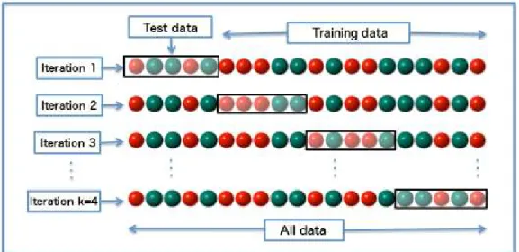
Figure 3.2 (Flöck 2016): An example of 4-fold cross validation in which 25% (1/4) of the data constitutes the validation set in each iteration. Each time, a different validation fold is used so that at the end of the 4 iterations every sample has been used once for testing and three times for training.
3.4 EVALUATING PERFORMANCE: METRICS
In order to compare the performance of different models between iterations we need to quantify it by using metrics. The most commonly used metric in classification tasks is accuracy, which measures the percentage of correct predictions. However, in our case where the dataset is imbalanced (relapse occurred in 22% of the patients, leaving a 78% of no relapse cases) this is not an appropriate metric. For instance, in an extreme case where relapse did not occur in 95% of cases, a predictive model that always predicted no relapse would achieve 95% accuracy, a very high score in spite of being a useless model. Furthermore, accuracy presumes that a mistake is equally worth in both cases, which is hardly the case in medical applications. For us, mistakenly predicting relapse will result in stronger chemotherapy, which is certainly undesirable as it has negative side effects; nevertheless, erroneously predicting no relapse can result in the death of the patient due to inadequate treatment. For these reasons we will opt for other metrics that provide a better insight.
In these scenarios, precision and recall are often preferred as they are more informative metrics. Recall, also known as true positive rate (TPR), is the percentage of positive instances that are correctly identified as such; i.e., the percentage of relapse cases that our model is able to predict.
21
𝑅𝑒𝑐𝑎𝑙𝑙 = 𝑇𝑃𝑅 = 𝑇𝑃 𝑇𝑃 + 𝐹𝑁
Where TP refers to true positives (accurate relapse predictions) and FN to false negatives (relapses missed by the model), therefore the sum of TP and FN constitutes the total number of positive instances (relapses).
On the other hand, precision is the percentage of accurate predictions for the positive class; i.e., the percentage of predicted relapses that were actually a relapse.
𝑃𝑟𝑒𝑐𝑖𝑠𝑖𝑜𝑛 = 𝑇𝑃 𝑇𝑃 + 𝐹𝑃
Where FP refers to false positive (wrong predictions of relapse), therefore the sum of TP and FP constitutes the total number of relapse predictions.
In summary, recall shows the proportion of relapses that our model is able to predict, and precision shows the accuracy of these predictions. These two metrics are combined in a single one called f1 which is the harmonic mean of both:
𝐹1 = 2 · 𝑅𝑒𝑐𝑎𝑙𝑙 · 𝑃𝑟𝑒𝑐𝑖𝑠𝑖𝑜𝑛 𝑅𝑒𝑐𝑎𝑙𝑙 + 𝑃𝑟𝑒𝑐𝑖𝑠𝑖𝑜𝑛
This type of mean penalises values of recall and precision that are too far from each other, leading to higher scores when both values are more similar. Translating precision and recall into a single metric allows to compare models more easily, and so we will use f1 when we have to compare tens or hundreds of models. However, there is a significant information loss since, as we said, there is an important different between failing to predict relapse (low recall) and wrongly predicting relapse (low precision). For this reason, whenever we present results we will show precision and recall along with the f1 score. Furthermore, we will assess more positively those models with higher recall over those with higher precision.
22
3.5 RESOURCES
The models and techniques used in this project have been implemented using python, which contains many helpful libraries for data science and machine learning. We have used pandas, for data handling; numpy, for computing vectors and matrices operations, matplotlib for data visualization, scikit-learn, which contains already implemented machine learning models and methods for data pre-processing, dimensionality reduction and model evaluation; imbalanced-learn, which uses the same interface as scikit-learn, and provides different techniques to deal with imbalanced data; TensorFlow, a low level deep learning framework; and Keras, built on top of TensorFlow to create a more accessible and higher level framework.
4. PRELIMINARY ANALYSIS AND DISCUSSION OF GENE EXPRESSION DATA
4.1 BRIEF SUMMARY OF DATASET CHARACTERISTICS
Here we restate some of the characteristic of our dataset that we have already mentioned, as we are about to discuss the challenges that these entail. First, the dataset is composed of 157 samples, which is a rather low number compared to most machine learning applications where at least thousands (sometimes up to millions) of samples are used. At the same time this is a common problem in biological datasets, where it is much more difficult to gather data; for instance, Golub et al. (1999), a reference study that worked on distinguishing ALL from AML (another type of leukemia) used only 72 samples.
A second frequent feature of these datasets is class imbalance, in our case 78% of patients do not experience relapse against a 22% who do; in the case of Golub et al. there was a 65% of AML patients and 35% of ALL. Finally, we have 11288 gene expressions of every patient (Golub et al. had 7129), which means we have almost 100 times more features than samples; this is known as high dimensionality (features can be though of as dimensions) and it is common to studies based on genetic information.
4.2 THE CHALLENGE OF LOW NUMBER OF SAMPLES
As we have previously discussed, machine learning being an empirical discipline means it relies very heavily on the available amount of data. Having more data results in a dataset that is more likely to be representative of the whole population. In other words, noise
23
(random fluctuations in features’ values) and outliers (samples that are outside usual boundaries due to measurement errors or very unlikely events) become less impactful and it is easier to recognise the overall pattern in the data.
4.3 THE CHALLENGE OF CLASS IMBALANCE
Class imbalance alone is not usually a big obstacle for achieving good performance. When there is enough data, just by adding class weights we can give more importance to prediction errors in the minority class, effectively making the model converge towards a more balanced solution. Other possibilities such as resampling techniques are also worth trying and can significantly improve performance in the minority class.
However, in our case there is a considerable limitation, namely, the lack of data addressed in the above section. This means that not only the minority class is underrepresented in the dataset, but also that there are so few minority class samples that it becomes extremely difficult to find a pattern within them. In other words, class imbalance, rather than being a challenge of its own, is exacerbating an already existing one: the scarcity of information to build a predictive model. We can add class weights to balance our loss function (and we will probably have to) but this will not add any new information about the minority class. We can also try oversampling techniques such as SMOTE (Chawla et al. 2002) or ADASYN (He et al. 2008), which generate synthetic samples of the minority class based on existing ones, hoping this will result in clearer patterns or boundaries between classes. However, these techniques work by picking a sample and applying linear interpolation between its same class nearest neighbours and itself to generate new samples; in a high dimensional space such as ours, samples are very sparsely distributed with large distances among them which usually leads to poor performance of nearest neighbours algorithms as well as poor accuracy of linear interpolation. An intuitive explanation can be given through a simple example of a balanced dataset with four samples and two features, one of which is absolutely unrelated to the output.
24
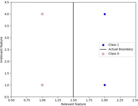
Figure 4.1: A balanced dataset of 4 samples with 2 features, one of them being unrelated to the output. Closest distance among same class samples (3 units) is larger than closest distance among opposite samples (1 unit) leading to poor performance of distance based methods such as nearest neighbours.
The purpose of this example is to visualize how irrelevant features equally contribute to determine the distance among samples, which in this case is leading to nearest neighbours belonging to opposite classes (note the different scales in the axes). If we go back to our high dimensional dataset where most of the features are almost certainly going to be irrelevant, we can clearly understand why nearest neighbours or linear interpolation are likely to yield poor results.
In summary, class imbalance exacerbates the lack of information about the minority class, complicating the job of finding clear patterns or boundaries. Using synthetic oversampling techniques, we can attempt to add more information about the minority class by including slightly modified versions of the original samples. However, these methods are distance-based and thus unlikely to perform well in a high dimensional dataset.
25
4.4 THE CHALLENGE OF HIGH DIMENSIONALITY
The main problem high dimensionality brings is the tendency to overfit. We can get an intuition of this issue by considering linear models, which are generally recommended for these types of datasets since they are less likely to overfit due to their simplicity. Recalling that we have 157 samples and 11288 features, we can consider each feature as a 157-dimensional vector. Given this, at most we will have 157 independent features, being the remaining 11131 features linear combinations of them (note that this linear relationship is ‘forced’ by the saturation of the 157-dimensional space, rather than being due to a real link among gene expressions). Having as many independent features as samples means we are guaranteed to have a solution for our classification problem regardless of the target function; but not only that, we can change freely the weights of any of the other 11131 features while maintaining the same output provided we make the necessary adjustments to the independent features’ weights. In summary, there is a 11131-dimensional space completely filled with solutions yielding perfect fits (we are not even considering approximated fits). Given the nature of the real problem we are trying to solve, we only expect an extremely tiny fraction of that space to contain actual solutions. Note that we are not looking for a unique solution since some variables might be correlated and we are aiming at good enough approximations, not perfect fits (there is hardly such thing as a perfect fit for real life problems); still, there is a gigantic haystack of possibilities that fit our training data but do not generalise hiding the few needles we are trying to find.
We can illustrate this by using a simple model such as logistic regression which is unlikely to overfit in common scenarios. Leaving the default parameters we obtain a perfect fit in the training set and a poor performance (0.37 f1 score) on cross validation; following the previous analogy we could say we have just encountered some hay (solutions that do not generalise). All of this suggests that dimensionality reduction (which could be thought of as hay removal) might play a key role in designing a successful model.
26
4.5 CHANGING PERSPECTIVE: A QUICK LOOK FROM THE BIAS-VARIANCE VIEWPOINT
As a side note that highlights the centrality of the bias-variance trade-off in machine learning, we can make a brief summary of the previous discussion from the bias-variance perspective. From this viewpoint, the problem of high dimensionality translates into a problem of complexity. A model with an extremely high number of features is ultimately a model with an extremely high complexity, resulting in low bias at the expense of very high variance, in other words, overfitting. The impact of the lack of data (which as already commented becomes exacerbated by class imbalance) can also be interpreted in similar terms. The lower the number of samples, the more impactful each individual sample is; therefore, the model will vary in higher degree when different samples are excluded/included from/in the model and training performance will be less representative of test performance, this is to say variance is high.
In conclusion, the three main challenges of this dataset contribute to increase variance resulting in very high probabilities of overfitting. Therefore, our aim will be to obtain very simple models as they are more likely to generalise. In this regard, we have seen that even the simplest models are prone to overfitting in such a high dimensional dataset; thus, high dimensionality can be considered as the main source of complexity in our model. Furthermore, distance based methods that could be used to deal with the class imbalance challenge are not suitable for high dimensional problems, which further stresses the importance of reducing dimensionality. Consequently, we will place special emphasis on dimensionality reduction.
5. EXPLORATORY PHASE
5.1 BRIEF ASSESMENT OF SEVERAL MODEL’S PERFORMANCE
Before starting working on dimensionality reduction and making models, it is always a good idea to do some tests on several out of the box models (a very brief description is given along with a reference for more rigorous explanations) from scikit-learn; this can give us an intuition of what seems to work best but also provides a baseline to which we can compare our further more elaborate models. We will use a grid search to explore different parameter settings for every model although we do not intend to be entirely exhaustive in this preliminary phase. Since we will have to train many different models
27
we will employ 10-fold cross validation to speed up the process. Every model is tested with equal and balanced class weights except Naïve Bayes, also standardization is used except on tree-based methods:
Naïve Bayes : assumes that the values of every feature for every class follow a Gaussian distribution, which allows to obtain a probability distribution that provides the likelihoods of these features. As a result, for any given value of a feature the likelihood can be obtained and used to calculate the probability of each class with the Bayes theorem. This algorithm does not have any hyperparameters to set (technically the priors could be altered but we will not do so).
Support Vector Machines (Cortes & Vapnik 1995): is a linear classifier that attempts to establish a boundary that maximizes the distance between the boundary itself (a hyperplane) and the closest samples from both classes. To obtain a non-linear classifier, we can use a kernel function that maps the original dimensional space to a higher dimensional space in which a hyperplane leads to a non-linear boundary back in the original dimensional space. We use the following hyperparameters:
o Kernels: control whether the decision boundary is linear or non-linear. There are three different kernels to obtain non-linear boundaries: sigmoid, rbf and polynomial. We will try all three as well as the linear option. o C: regulates the complexity of the model, lower values resulting in
simpler models. The default value is 1, we will try values ranging from 0.01 to 100
o Gamma: only used for non-linear kernels. It is another form of regulating the complexity of the model, with lower values resulting in simpler models. By default, it is set to 1/n where n is the number of features. We will use values range from 1e-5 to 1e-3.
Logistic regression (Cox 1958): assigns weights to every feature and sums all these contributions adding a bias term. This result is used as the input of a sigmoid function, which maps every real number into a number between 0 and 1, which can be thought of as the probability of a sample belonging to a certain class. During training, the logistic regression model modifies the weights and bias in such a way that the probabilities of each sample belonging to a class are closest to the actual label. We use the following hyperparameters:
28
o Penalty: can be set to l1 or l2 (these terms will be explained in section 5.3) but they cannot be combined. We will use both.
o C: same as in support vector machines. We will try values ranging from 0.01 to 100.
Stochastic Gradient Descent Classifier (SGD) (Zhang 2004): uses an optimization procedure known as stochastic gradient descent for minimizing the prediction error of different classifiers. In our case, we set the ‘Loss’ hyperparameter to ‘log’, resulting in a logistic regression model. The reason we do this is that this implementation of logistic regression allows to combine l1 and l2 penalty as in Elastic Net through the ‘L1_ratio’ hyperparameter. o L1_ratio: Values range from 0 (just l2 penalty) to 1 (just l1 penalty). The
limit cases 0 and 1 are not included as it would be redundant with the other implementation of logistic regression.
o Alpha: controls complexity in the same way as C. Values are set ranging from 0.1 to 20.
Decision Tree (Breiman et al. 1984): the decision tree starts with a node containing all samples and iteratively splits each parent node into two child nodes, attempting to separate samples from different classes, until every leaf (final node) contains same class samples. We use the following hyperparameters:
o Information criterion: determines the criterion used to decide what split best separates the samples we try both gini and entropy.
o Minimum weighted fraction: this parameter regulates tree pruning, i.e., avoids growing full trees. When the weighted sum of samples in a node falls below this fraction (fraction of the total weighted sum of samples) no more splits are made. Therefore, this parameter, unlike the commonly used maximum depth, takes into account class weights. We will use values ranging from 0.01 to 0.2.
Random Forests (Breiman 2001): use bagging (explained in section 7.2) to make an ensemble of decision tree classifiers. Each tree, rather than looking at the entire set of features for making splits, only considers a smaller randomly chosen subset. We use the following hyperparameters:
o Same parameters as Decision Tree except for the addition of a 0 minimum weighted fraction at leaf option to allow for growing full trees.
29
o Number of estimators: number of trees employed. We use values ranging from 10 to 200
o Number of features: size of the subsets of features that are given to the trees. By default is the square root of the number of features in our dataset. We try values ranging from 0.005 and 0.1
o Bootstrapping: whether or not to use bootstrap samples. We try both. Extremely Randomized Trees (Geurts et al. 2006): work very similarly to
random forests. The only difference is that when considering the best split, a random threshold (instead of the most discriminative one) is given to each candidate feature.
o Same parameters as Random Forests
AdaBoost (Freund & Schapire 1997): fits a sequence of decision trees, each time giving more importance to those samples that were misclassified by the previous tree. Final predictions are a weighted average of the predictions made by each tree. We use the same hyperparameters as random forest except for the learning rate:
o Learning rate: indirectly controls the complexity of the model. We try values ranging from 0.1 to 5.
For every model, now we show those combinations of parameters that resulting in the best f1 score along with the 10-fold cross validation results:
Naïve Bayes:
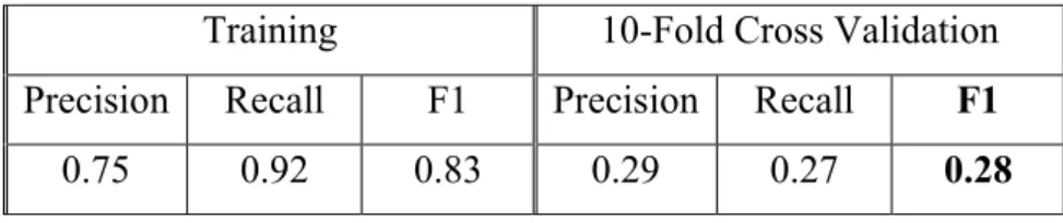
Table 5.1 Naïve Bayes Training and Validation Performance
Training 10-Fold Cross Validation Precision Recall F1 Precision Recall F1 0.75 0.92 0.83 0.29 0.27 0.28
Support Vector Machines:
Table 5.2 Support Vector Machines (No Class Weights, Sigmoid Kernel, Gamma=0.001, C=10) Training and Validation Performance
Training 10-Fold Cross Validation Precision Recall F1 Precision Recall F1 0 0 0 0 0 0
30
Logistic Regression: balanced class weights, l1 regularisation and C=0.1
Table 5.3 Logistic Regression (Balanced Class Weights, L1 Penalty, C=0.1) Training and Validation Performance
Training 10-Fold Cross Validation Precision Recall F1 Precision Recall F1 0.63 1 0.78 0.41 0.81 0.55
Stochastic Gradient Descent Classifier: balanced class weights, l1_ratio=0.5, alpha=2
Table 5.4 Stochastic Gradient Descent Classifier (Log Loss, Balanced Class Weights, L1_Ratio = 0.5, Alpha = 2)
Training 10-Fold Cross Validation Precision Recall F1 Precision Recall F1 1 1 1 0.33 0.54 0.41
Decision Tree: balanced class weights, entropy criterion and 0.2 as minimum weighted fraction at leaf.
Table 5.5 Decision Tree (Balanced Class Weights, Entropy Criterion, 0.2 Minimum Weighted Fraction at Leaf)
Training 10-Fold Cross Validation Precision Recall F1 Precision Recall F1 0.78 0.81 0.79 0.23 0.31 0.26
Random Forests: balanced class weights, entropy criterion, 0.2 as minimum weighted fraction at leaf, 10 estimators and using 1% of features per bag without bootstrapping samples.
31
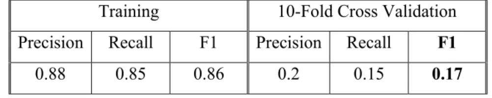
Table 5.6 Random Forests (Balanced Class Weights, Entropy Criterion, 0.2 Minimum Weighted Fraction at Leaf, 10 Estimators, 0.01 Number of Features, No Boostrapping) Training and Validation Performance.
Training 10-Fold Cross Validation Precision Recall F1 Precision Recall F1 0.88 0.85 0.86 0.2 0.15 0.17
Extremely Randomized Trees: balanced class weights, gini criterion, 0.1 as minimum weighted fraction at leaf, 10 estimators and using 10% of features per bag without bootstrapping samples.
Table 5.7 Extremely Randomized Trees (Balanced Class Weights, Gini Criterion, 0.1 Minimum Weighted Fraction at Leaf, 10 Estimators, 0.1 Number of Features, No Boostrapping) Training and Validation Performance.
Training 10-Fold Cross Validation Precision Recall F1 Precision Recall F1 1 1 1 0.30 0.12 0.17
AdaBoost: balanced class weights, entropy criterion, 0.15 as minimum weighted fraction at leaf, 10 estimators and 1 learning rate.
Table 5.8 Adaboost (Balanced Class Weights, Entropy Criterion, 0.15 Minimum Weighted Fraction at Leaf, 10 Estimators, 1 Learning Rate) Training and Validation.
Training 10-Fold Cross Validation Precision Recall F1 Precision Recall F1 1 1 1 0.33 0.27 0.30
32
5.2 BRIEF ANALYSIS OF RESULTS
The first fact that clearly stands out is the high performance of logistic regression in comparison to the rest of the models. This will now become our baseline model and the focus of our attention in further analysis but now we will take quick look at the other algorithm’s performance.
After a general overview, we see that all models are strongly overfitting (results are much better on the training set than on cross validation) even the simplest ones, which seems to back our previous analysis in which we identified variance as the main source of error. Looking more closely we see that tree-based methods do not seem to handle this dataset well. We cannot be entirely sure of this fact since our search was not completely exhaustive, and also their behaviour might improve significantly after dimensionality reduction; still, we will not expect high results from these types of algorithms. It is interesting how Random Forests and Extremely Randomized Trees are achieving such poor performances, worse than AdaBoost and even a single Decision Tree. This is surprising because a priori we would expect these algorithms to be suitable for our dataset, since they are specifically designed to reduce variance. They mainly achieve this by using bagging and by limiting the number of features that each individual tree uses. Interestingly enough, in both cases bootstrapping is not preferred; therefore, bagging was not being helpful in reducing variance. This might be due to the fact that bootstrap samples only contain about 2/3 of the original data, reducing the number of instances used for training in an already small dataset; furthermore, since we used cross validation instead of out of bag samples for testing, this problem becomes exacerbated. As we have mentioned earlier, training sets favour high variance, so the benefits bagging brings may be surpassed by the negative effects of reducing the effective size (in terms of number of different samples) of the training set. With this said, once again we cannot make these conclusions definitive, although we cannot ignore the valuable insights we have gained either.
On another order of things, Stochastic Gradient Descent, which is implementing a slightly different version of Logistic Regression is achieving the second-best result, leading us to believe that this type of model is the most adequate for this dataset. Finally, the awful performance of Support Vector Machines (it is classifying all samples as majority class) across a reasonable range of hyperparameters is a surprising outcome that might deserve further attention.
33
5.3 ANALYSIS OF THE LOGISTIC REGRESSION MODEL
Now we turn to the Logistic Regression model whose performance clearly stands out in comparison to the rest and thus will become our baseline model. What is rather interesting is that l1 penalty seems to make a significant difference; indeed, the Stochastic Gradient Descent Classifier which is also implementing logistic regression but with different penalties has a considerably lower performance. Explaining l1 and l2 regularisation can help understanding the reason behind this.
Baseline model: Logistic Regression (balanced class weights, l1 penalty and C=0.1):
Table 5.9 Baseline Model: Logistic Regression (Balanced Class Weights, L1 Penalty, C = 0.1).
Training Leave One Out Cross Validation Precision Recall F1 Precision Recall F1
0.63 1 0.78 0.47 0.81 0.59
Baseline model with l2 penalty instead of l1:
Table 5.10 Baseline Model with L2 Penalty: Logistic Regression (Balanced Class Weights, L2 Penalty, C = 0.1).
Training Leave One Out Cross Validation Precision Recall F1 Precision Recall F1
0.86 0.92 0.89 0.30 0.65 0.41
L2 penalty includes the squared values of the weights in the loss function, heavily penalising high weights but almost ignoring low values; on the contrary, l1 penalty uses the absolute values of weights, meaning that low values will still be considered and attempted to minimise, pulling them towards 0. In other words, l1 penalty makes 0 the weight of those features that are not meaningful enough, while maintaining those who are more valuable for the classification task. In fact, if we look at the coefficients of this classifier we see that only 20 of them are not 0. In conclusion, l1 penalty incorporates feature selection into the regression model. As we previously mentioned, dimensionality reduction is likely to play a crucial role in obtaining a successful model, so it is not
34
surprising that the only method that incorporates some type of feature selection clearly outperforms the rest.
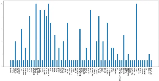
It should be noted that despite the model simplicity: a regularised linear model using 20 features, it is still significantly overfitting, which gives us an idea of how difficult it is to reduce variance in this dataset. Anyway, feature selection seems to be the key to the good model performance, so we will analyse it to gain more insight. First, we would like to know whether the same features are being selected every time, which would mean that those features are truly the most informative and we could focus on them for future models. We can store the selected features in each iteration of 10-fold cross validation, and then plot the frequencies with which they appear, obtaining the following result.
Figure 5.1: Number of times each gene is selected over 10 iterations of cross validation.
We can see that a significant number of features are only used by the model in one iteration of cross validation. This can be due to two reasons: some of these features are highly correlated, meaning that the model is not able to clearly pick one over the other as they provide similar information; or these features are only relevant for a particular subset of the training set (the one corresponding to that cross-validation iteration), in other words, they are the result of overfitting and they lack generalisation. We can quickly decide which hypothesis is more accurate by plotting the correlation matrix:
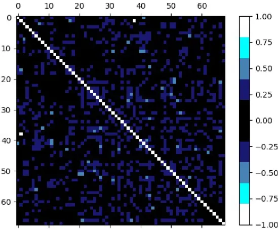
35
Figure 5.2: Plot of the correlation matrix (of the features that are at least selected once) where each square represents each of the correlation coefficients in the matrix. Colours cover 0.2 intervals in absolute value and allow to display the value of each correlation coefficient. There are no white or light blue squares (outside of the main diagonal) meaning that all correlation coefficients in absolute value are below 0.6
Correlations among features are not strong, therefore we discard the first hypothesis concluding that those features which were used in just a few of the cross-validation iterations were selected out of chance and not due to a true relationship with our labels. Now that we have seen that a significant number of the selected features are not actually relevant two questions arise. First, are those features with high frequencies truly informative or where they also chosen out of chance? Second, where can we establish the threshold between relevant and irrelevant features based on their frequencies? To answer these questions, we can run 10-fold cross-validation with random seed 100 times, totalling 1000 trials, and plot the results in the same manner as before:
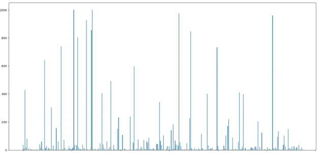
36
Figure 5.3: Number of times each feature is selected over 1000 trials. There is not enough space to make labels readable and we are not interested in identifying any particular feature but in the overall picture of frequencies; therefore labels are not shown.
Looking at the above figure we see a similar picture as before but at a higher scale. Initially, we could say that we can now be more certain that those features that have high frequencies are actually relevant, since they are not only selected for a particular cross validation split, but across a wide range of subsets made with 90% of the training data (since it is 10-fold cross-validation). However, our second concern (what threshold should be used to decide between relevant/irrelevant features) has not been resolved as there is no clear gap between high and low frequencies, bringing in another perspective that casts doubt about the validity of our results.
We were expecting that as we run more trials, our model would always select the same relevant features while changing in each iteration the chosen irrelevant features. This would result in a plot in which a few features clearly stand out, with a significant gap separating them from the rest. However, in our figure, instead of a gap, there is continuity between low and high frequency values. This means, for instance, that some features are relevant for 40% of the subsets but not for the remaining 60%; therefore, they are not truly meaningful, they happened to be correlated with the output out of chance for those particular subsets. We can now look at features that are selected for 60% or 80% of the models and follow the same reasoning. Then, how sure can we be that features selected
37
100% of the time are actually relevant and did not happened to be correlated with the output out of chance?
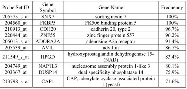
Table 5.11 10 Most Frequently Selected Genes by the Baseline Model.
Probe Set ID Symbol Gene Gene Name Frequency 205573_s_at SNX7 sorting nexin 7 100%
204560_at FKBP5 FK506 binding protein 5 100% 210913_at CDH20 cadherin 20, type 2 96.7% 220444_at ZNF55 zinc finger protein 557 96.2% 205013_s_at ADORA2A adenosine A2a receptor 91.4% 205539_at AVIL advillin 86.7% 211549_s_at HPGD hydroxyprostaglandin dehydrogenase 15-(NAD) 83.4% 204749_at NAP1L3 nucleosome assembly protein 1-like 3 80.1% 203367_at DUSP14 dual specificity phosphatase 14 75.9% 213798_s_at CAP1 CAP, adenylate cyclase-associated protein 1 (yeast) 71.6%
Finally, it should be noted that the whole training set has been used to rank features according to their relevancy. Thus, cross validation will not give us a good estimate of generalization performance. We can use the 10 most frequently selected attributes (we choose 10 because those are the genes with a frequency over 70%) to make a logistic regression model and after a some tuning we will get the following results:
Table 5.12 Logistic Regression Model (Balanced Class Weights, L2 Penalty, C = 30) With 10 Selected Genes.
Training Leave One Out Cross Validation Precision Recall F1 Precision Recall F1
0.95 0.91 0.93 0.73 0.85 0.79
In spite of overfitting, cross validation results are considerably good but cannot be compared against those of the baseline model since the feature selection process was made based on the entire training set. As a result, only the results in the test set will be an accurate estimate of generalization.
38
5.4 CONCLUSION
Feature selection performed by our baseline model seems to provide good results, although the generalization of these results is in question until we reach the testing phase and obtain more information. Therefore, we will continue with our initial plan and focus on dimensionality reduction.
6. DIMENSIONALITY REDUCTION
6.1 ESTABLISHING A TARGET NUMBER OF DIMENSIONS
When attempting dimensionality reduction, it is convenient to have an idea of the number of dimensions that is the most appropriate for the problem in hand. In our case, we are aiming at having less features than samples, since as we have discussed generalisation is hard to obtain when this is not the case. Ideally, we would like to have less than 20 features (this value is approximate and based on intuition as there is no clear rule determining the optimal number of features) so that we obtain a very simple model that is unlikely to overfit. At the same time, compressing 11288 features into just 10-20 is not an easy task and it might be not even possible. As in any case, the strategies chosen to achieve this goal will greatly determine the probabilities of success.
6.2 UNSUPERVISED VS SUPERVISED DIMENSIONALITY REDUCTION
Unsupervised dimensionality reduction tries to achieve a lower dimensional representation of the features while maintaining the inner structures and relationships; while its supervised counterpart aims at selecting a set of relevant features discarding all the attributes that seem unrelated with the output. With these ideas in mind, we can start comparing both methods.
On one hand, supervised approaches are more likely to overfit for the following reason. They select features based on how related they are with the output in the training set, which will lead to those attributes that give better performance in the training set being selected. As a consequence, training results may be overly optimistic and not reflect reality. This is the case with our baseline model, which is overfitting despite its great simplicity, as it is performing a form of embedded supervised feature selection. On the
39
contrary, unsupervised approaches minimize the amount of information they use from the training set by disregarding output labels often leading to more generalizable results.
On the other hand, the same reason that leads to an advantage of unsupervised methods can turn into a downside in cases where most of the features are irrelevant like ours. In these scenarios, unsupervised approaches will be heavily limited by the requirement to preserve internal relationships among irrelevant features, even though these have no effect on our predictive model. Consequently, supervised methods can be more powerful (in terms of achieving greater reductions in dimensionality) in these circumstances as they can identify non-informative attributes and discard them.
Since there is no clear conclusion from this discussion we will attempt both strategies.
6.3 SUPERVISED DIMENSIONALITY REDUCTION
6.3.1 Decision Tree Based Methods: Feature Importance
When using Decision Tree based methods we can get an estimate of each feature’s importance by considering how good they are at reducing impurity (breaking a two-class group into two single class groups) in each node. Then the least important features can be removed from the model. Features’ importance is usually obtained using Random Forests, but this does not necessarily have to be the case. Unfortunately, Decision Tree based methods perform rather poorly in our dataset, so the importance they assigned to each feature is not meaningful.
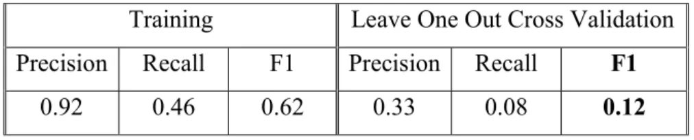
6.3.2 Linear Discriminant Analysis (LDA)
Most of the supervised dimensionality reduction techniques are based on classifiers and this is not an exception. As its name implies, LDA (Hastie et al. 2008) uses linear decision boundaries to classify samples; however, what makes it interesting for us is that it provides the most discriminative directions in our dataset, in other words, it allows to perform dimensionality reduction. We can test the model predictions to get an idea of how good LDA works in our dataset:
40
Table 6.1 Linear Discriminant Analysis Training and Validation Performance.
Training Leave One Out Cross Validation Precision Recall F1 Precision Recall F1
0.92 0.46 0.62 0.33 0.08 0.12
Given such poor results, we cannot rely on how this algorithm classifies the most discriminative directions and so we will move onto other approaches.
6.3.3 F-test Based Feature Selection
This technique consists in using One-Way ANOVA (Analysis of Variance of a single feature) (Heiman 2001) in order to discern whether the difference in the mean value of a feature from one class to another is statistically significant. In our case, for every gene, we want to see if the mean level of expression in relapse samples is significantly different than the mean level of expression in no relapse samples.
This method has two main limitations, namely it performs univariate feature selection and it is based on many assumptions including linearity and normally distributed (within class) gene expression levels. Performing univariate feature selection means that we are only considering relations between each feature and the output, disregarding relationships among features; which can result in our model having redundant features (features that contain the same information). This is not a considerable disadvantage as we can always look at the correlation matrix of the selected features and discard those that are redundant. Similarly, the assumptions made by One-Way ANOVA are not a strong downside in our case, since they also lead to simpler models with less variance. We can plot the F-statistic we obtain after applying in this technique, sorting values in descendent order:
41
Figure 6.1: Plot of the F values of every gene expression in descendent order.
As we had expected, most gene expressions are uncorrelated with relapse whereas a few are truly significant. There is a noticeable inflexion point that separates these two groups, although it is hard to see how many features constitute each side. For this reason, we will zoom in by only considering the 2000 most relevant features:
Figure 6.2: Plot of the F values of the 2000 most relevant genes.
INFLEXION POINT
42
We can see the inflexion point is closer to 0 than to 250 but it is still hard to identify a precise value. Therefore, we zoom again, only showing the 500 most significant genes:
Figure 6.3: Plot of the F values of the 500 most relevant genes.
Finally, we can see that the division point is at around 50 genes. In other words, we can say that there are approximately 50 relevant genes according to the F-test feature selection. We can now look at the correlation matrix whether this univariate approach is including too many redundant attributes.
43
Figure 6.4: Correlation matrix of the 50 features selected according to the F-test.
All correlations are below 0.8 (in absolute value), and only 4 are above 0.7. Therefore. there is not a problem of redundancy and we can continue with our study. To test this feature selection process in a model, we do not just select the 50 genes with the highest score in the whole training data as this would undermine the validity of cross validation results. Instead, we perform feature selection in each iteration of cross validation, using each training fold rather than the entire training set. After trying several logistic regression models with different parameters settings (l1 and l2 penalties across C values between 0.01 and 100), we obtain this model:
Logistic Regression: balanced class weights, l2 penalty and C=30.
Table 6.2: Logistic Regression (Balanced Class Weights, L2 Penalty, C= 30) with 50 Genes Selected by ANOVA.
Training Leave One Out Cross Validation Precision Recall F1 Precision Recall F1