Multi-level spherical wave expansion for fast near-field to far-field transformation

Multi-Level Spherical Wave Expansion for Fast

Near-Field to Far-Near-Field Transformation

Fernando Rodríguez Varela, Manuel Sierra Castañer, Belén Galocha Iragüen

Universidad Politécnica de Madrid Av. Complutense nº 30, Madrid, Spain {f.rodriguezv, manuel.sierra, belen.galocha}@upm.es

Abstract—Traditional near-field to far-field transformation algorithms based on modal expansion are unable to deal with arbitrary measurement surfaces. To approach these problems, a matrix inversion method can be used to retrieve the spherical wave expansion (SWE) of the antenna under test (AUT) fields. Modeling the antenna with a set of multiple SWEs centered at arbitrary points over its surface offers a flexible approach for the solution of field transformation problems over arbitrary surfaces. The coefficients of each SWE are obtained using an iterative inversion approach where the matrix-vector products can be replaced by multilevel operators based on recursive aggregations and interpolations of the partial SWE fields, reducing the computational complexity from 𝑶(𝒇𝟒_{) to 𝑶 𝒇}𝟐_{𝐥𝐨𝐠 𝒇 . The}

proposed algorithm is tested using synthetic data and measurements showing good scalability and reduced transformation error.

I. INTRODUCTION

Spherical near-field antenna measurements constitute one of the most powerful and accurate techniques for antenna pattern characterization [1]. The analytical spherical wave expansion (SWE) formulation allows the implementation of extremely efficient algorithms based on the application of Fast Fourier Transform techniques for the transformation of the measured field to the far-field pattern. Traditionally, spherical near-field to far-near-field transformation algorithms have focused on the processing of equi-spaced spherical acquisition surfaces measured with mono-mode probes [2].

New communication systems have prompted the development of new algorithms capable of dealing with new measurement schemes, where the fields are measured over arbitrary surfaces different from spheres, with irregular sampling schemes and/or multimode probes with arbitrary orientations [3][4]. In these scenarios, the application of traditional modal techniques is infeasible, as spherical waves orthogonality no longer holds. A usual way of addressing this problem is to take an equivalent sources approach, where the antenna under test (AUT) is modeled with an equivalent source representation. The representation is found solving a linear system of equations constructed from the measurement points. Then, the far-field of the representation is evaluated asymptotically to obtain the AUT radiation pattern. This process is outlined in Figure 1.

The most common sources representation are magnetic and electric currents [5], but the antenna can also be modeled with

an unknown spherical wave expansion that is found solving an equation system [4]. The main drawback of these type of approaches is the poor computational performance and scalability. Due to the high number of unknowns involved, the system of equations must be solved iteratively, where each iteration involves a set of matrix-vector products with a computational complexity (CC) of 𝑂((𝑘𝑟 ) ), being 𝑟 the antenna minimum sphere radius and 𝑘 the wave number.

Near-field to far-field transformation basic principle

To improve the computational complexity of equation systems, multilevel approaches are used, in which the matrix-vector products of the iterative matrix inversion are replaced by fast operators that bring the CC down to 𝑂((𝑘𝑟 ) log(𝑘𝑟 )). This improvement is achieved by subdividing the problem in a recursive fashion, as it is done in Multi-Level Fast Multipole Method [6] and Fast Physical Optics [7][8].

the multilevel principles of Fast Physical Optics on each iteration of the matrix inversion algorithm. A recursive interpolation/aggregation process is performed to reduce the problem computational complexity from the conventional

𝑂((𝑘𝑟 ) ) to 𝑂((𝑘𝑟 ) log(𝑘𝑟 )).

The structure of this paper is as follows. In Section II, the basic theory of the multi-level spherical wave expansion is presented. In section III, the approach is validated based on simulations of antenna fields, leaving the verification with real measured data for section IV. Section V concludes this paper.

II. MULTI-LEVEL SPHERICAL WAVE EXPANSION

A. Multiple spherical wave expansion representation

Consider an antenna located at the center of a coordinate system. The field radiated by the antenna can be expressed in terms of a spherical wave expansion, centered at the origin of the coordinate system [1]:

𝐸⃗(𝑟, 𝜃, 𝜑) = 𝑄 𝐹⃗( )(𝑟, 𝜃, 𝜑) (1)

This system is referred as the global coordinate system. Now, the spherical wave expansion can be centered at an arbitrary point. To do so, a local coordinate system centered at a point

(𝑥 , 𝑦 , 𝑧 ) is defined having its main axis parallel to the global one, i.e. (𝑥 = 𝑥, 𝑦 = 𝑦, 𝑧̂ = 𝑧̂). The SWE centered in this local system is given by:

𝐸⃗(𝑟, 𝜃, 𝜑) = 𝑄 𝐹⃗( )(𝑟 , 𝜃 , 𝜑 ) (2)

being (𝑟 , 𝜃 , 𝜑 ) the coordinates of point (𝑟, 𝜃, 𝜑) in the local coordinate system (𝑥 , 𝑦 , 𝑧 ).

More coordinate systems with its local SWEs can be defined. The antenna field can be expressed as the aggregation of all the contributions of each SWE:

𝐸⃗(𝑟, 𝜃, 𝜑) = 𝑄 𝐹⃗( )(𝑟 , 𝜃 , 𝜑 ) (3)

Each SWE can be truncated to a given 𝑁 index that depends on the antenna size and the distribution of the partial SWEs over the antenna volume. However, by the equivalence theorem, only SWEs centered at points over a surface enclosing the antenna are needed.

If the partial SWE centers are uniformly distributed, the truncation index can be the same for all of them 𝑁 = 𝑁. The actual index 𝑁 will depend on the spacing between SWEs. The more separated they are, a higher 𝑁 is needed to model the AUT field variations adequately. Figure 2 depicts a schematic representation of the introduced formulation.

Summation in (3) can be expressed as a matrix-vector product:

𝐸 = 𝐶𝑄 (4)

where 𝐸 and 𝑄 are column vectors that contain the AUT radiated field and spherical coefficients of each expansion respectively, whereas 𝐶 is the coupling matrix that contains the spherical wave vectors of (2) and the required coordinate system transformations to obtain the radiated field by all spherical wave expansions.

𝐸 =

⎝ ⎜ ⎜ ⎛

𝐸 (𝑟 , 𝜃 , 𝜑 ) 𝐸 (𝑟 , 𝜃 , 𝜑 ) 𝐸 (𝑟 , 𝜃 , 𝜑 )

⋮

𝐸 (𝑟 , 𝜃 , 𝜑 )⎠ ⎟ ⎟ ⎞

𝑄 =

⎝ ⎜ ⎜ ⎜ ⎛

𝑄, , ⋮ 𝑄, , 𝑄, ,

⋮ 𝑄, , ⎠

⎟ ⎟ ⎟

⎞ ₍₅₎

Modeling of the AUT fields with a single SWE (a) and with several local SWEs (b)

B. Multiple SWE near-field to far-field transformation The multiple SWE constitutes an equivalent representation of the AUT fields so it can be used to perform near-field to far-field transformations. If the AUT electric far-field is measured in a set of points over a surface, a linear system of equations using the matrix notation of (4) can be formulated, with 𝐸 being the

(a)

measured fields arranged in a column and 𝑄 the unknown coefficients of all local SWEs. To reach a valid solution some degree of overdetermination is required in the system, i.e. more sampling points than unknowns measured for two orthogonal polarizations. There are no further constraints for the solution of the problem so any arbitrary surface enclosing the antenna can be used as long as it provides good problem conditioning.

The least squares solution of the problem is given by:

𝑄 = (𝐶 𝐶) 𝐶 𝐸 (5)

where𝐶 denotes transpose conjugated. Direct inversion of

(𝐶 𝐶) is not feasible in problems with high number of unknowns, so an iterative method such as Conjugate Gradient (CG) [9] is used. Once the coefficients of all spherical wave expansions are obtained, they can be evaluated at far-field using the asymptotic expression of the spherical wave functions obtaining the AUT radiation pattern straightforwardly.

C. Multi-level SWE field computation

The bottleneck of the proposed transformation algorithm is located in the matrix-vector products of each step of the iterative inversion algorithm. This is a well-known limitation of electromagnetic inversion problems. The number of spherical waves needed to model the AUT field grows with 𝑂(𝑘𝑟 ) . The number of equations must grow proportionally to the number of unknowns, i.e. 𝑂(𝑘𝑟 ) scalability too. Therefore, the computational cost of performing a matrix-vector product is

𝑂(𝑘𝑟 ) .

To reduce computational complexity the matrix-vector products are replaced by operators that make the calculations “on the fly”. To do so, we note that on each step of the iterative algorithm the radiated field by a set of spherical coefficients 𝑄

must be calculated. The algorithm stops when this radiated field is similar enough to the measured field. Therefore, a fast operator must be devised to calculate the fields radiated by a set of spherical waves expansions. We denote the application of this operator as 𝐹().The purpose of this operator is to replace the computationally intensive task of performing the product of (4):

𝐸 = 𝐶𝑄 → 𝐸 = 𝐹(𝑄) (6)

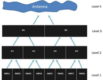
Fast Physical Optics [7] is a numerical method to integrate physical optics (PO) [10] currents with reduced computational complexity. It is based on a multi-level domain decomposition in which fields are calculated for small domains in a coarse grid of points and then aggregated and interpolated recursively to a finer grid. The same principle can be applied for this case, but instead of integrating PO currents, spherical wave fields are aggregated.

Figure 3 shows a simplified scheme of a multi-level decomposition of an antenna in one dimension. The lowest level shows that the antenna has been modeled using 8 SWEs centered along the antenna shape. The partial fields of each SWE show smoother variations than the total antenna field, so they can be calculated in a coarse grid of points. On the next level, the SWEs have been grouped in pairs and the fields of each pair member are aggregated. As a result, the aggregated fields will have now stronger oscillations, so the field sampling rate must be doubled with interpolation before the summation. This

interpolation-aggregation step is repeated until the field of the total antenna is obtained in the last level.

This calculation is equivalent to performing the 𝐶𝑄 product inside the iterative algorithm. The difference lies in the number of operations required to perform the calculations. On each level of the multi-level scheme (operator 𝐹() ), interpolations/summations are performed over the measurement surface giving a cost of 𝑂((𝑘𝑟 ) ). Since the total number of levels in the recursive domain decomposition grows at logarithmic rate, the total computational complexity of the calculation is 𝑂((𝑘𝑟 ) log(𝑘𝑟 )), as compared with the

𝑂((𝑘𝑟 ) ) of the matrix vector product 𝐶𝑄.

Schematic view of an antenna multi-level domain decomposition in one dimension

III. NUMERICAL RESULTS AND DISCUSSION

The purpose of this section is to verify the functionality of the proposed arbitrary-surface near-field to far-field transformation algorithm using a simulated example. Considered is a distribution of 170 Hertzian dipoles randomly placed at plane 𝑧 = 0 with an approximate size of 150×150 mm, operating at 5 GHz. The field radiated by this distribution is analytically computed over an arbitrary surface enclosing it. For this case an ellipsoid has been used as measurement surface with semi-axis (𝑎 = 490, 𝑏 = 470, 𝑐 = 240) and a sampling of 16 points in 𝜃 and 32 in 𝜑. At each point two orthogonal polarizations are measured. The problem geometry has been depicted in Figure 4.

A. Matrix inversion example

16×32×2=1024 equations. The equation system is solved iteratively using Conjugate Gradient with a vector of zeros as initial guess. At each iteration the norm of the residual is calculated as follows:

𝑟 =‖𝐶 𝐸 − 𝐶 𝐶𝑄 ‖

‖𝐸‖ (7)

being 𝑄 the solution estimation at the 𝑘th iteration. The algorithm is stopped when a residual of 10 is reached. Finally, the obtained mode distribution is evaluated at the far-field to obtain the AUT radiation pattern.

Test problem geometry

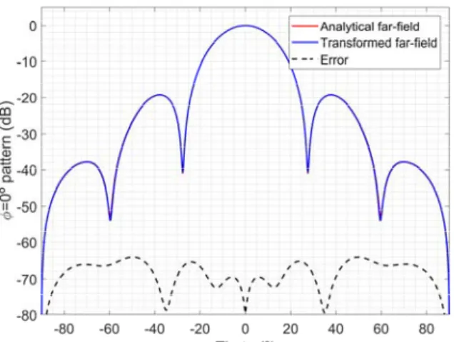
The transformed far-field pattern is depicted in Figure 5. This field has been compared with the analytical far-field pattern of the dipole distribution. The two graphs show excellent agreement being the error of the order of -70dB due to the low value of the residual.

B. Multi-level operator

Now that the functionality of the multiple SWE has been demonstrated, the matrix-vector products of the iterative algorithm are replaced by the fast multi-level operator 𝐹()

presented in section II. To show the scalability of the multi-level approach, simulations are performed for frequencies up to 80 GHz. The measurement sampling rates are increased accordingly, as well as the number of SWEs and levels of the multilevel structure. For example, at 5 GHz 3 levels will be used to group all SWEs, this corresponds to the case of Figure 3 but in 2 dimensions. At 10 GHz the number of SWEs and the sampling rate are double on each dimension, and 4 levels are used. For simplicity, the frequency will be increased in powers of two (5,10,20,40,80 GHz)

The computational gains of the multilevel approach lie in the coarser sampling of the partial SWEs. On each level ascension, the sampling rate is doubled on each dimension. The initial sampling rate for the lowest level must be selected as a compromise of calculation time and accuracy. To asses this aspect the following experiment is performed. The result of the

matrix-vector product is compared with the application of the multilevel operator for a given set of sampling rates. This can be expressed as:

𝜖 = 𝐶𝑄 − 𝐹 (𝑄) (8)

where an index 𝑠 has been added to the operator to denote the sampling rate used.

Comparison of the transformed far-field with the analytical solution

Figure 6 depicts the results of the proposed experiment. The calculated field using the matrix-vector product 𝐶𝑄 at one iteration has been plotted in the blue curve. The rest of the curves show the error between this reference field and the ones obtained using the multilevel operator for 3 different base sampling rates. Table I lists the main parameters of each sampling rate, along with the simulation time taken by the application of the multilevel operator. These sampling rates are referred to the lowest level. To perform the interpolations cubic splines have been used but other types of interpolation schemes have been explored for this type of problems [8].

TABLE I. SAMPLING RATE PARAMETERS

Sampling rate Samples in 𝜽 Samples in 𝝋 Calculation time

𝑠 = 1 6 12 4 s

𝑠 = 2 9 18 6.5 s

𝑠 = 3 12 24 7.1s

Calculation errors for three different sampling rates of the multi-level operator

Evolution of the CG residual at 3 different frequencies

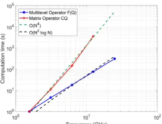
A comparison of the scalability between the matrix-vector product and the multi-level operator has been performed. It is noteworthy that all algorithms have been implemented in MATLAB so there is a huge handicap in performance between the matrix-vector products that are native operations, and the proposed multi-level implementation lacking code vectorization and optimization. However, these are just considerations of absolute computation time, as algorithms scalability is not affected by this. Therefore, for better comparison between the two operators, the computation time required to perform one iteration of the multilevel approach has been compared with the time required to populate matrix C in the matrix-vector product approach.

Figure 8 shows the results of the time comparison between the two approaches. To obtain the curves, the frequency of the random dipole test case has been varied between 5 and 80 GHz. Two curves showing a frequency scalability of 𝑓 and 𝑓 log 𝑓

have been superposed, showing good agreement with the curves of the matrix and multi-level operator, respectively.

Computational complexity of the two operators

Finally, to demonstrate the accuracy of the multilevel approach in a complete near-field to far-field transformation problem, the iterative algorithm has been applied at 80 GHZ using multilevel operators for the same geometry of Figure 4. The obtained results are depicted in Figure 9, where the error has increased up to -50 dB due to the interpolations. The complete transformation took 8 hours on an Intel Core i5 2.5 GHz PC. In this case, a comparison with the matrix approach was impossible to make due to the high memory requirements of this approach.

Comparison of the transformed far-field with the analytical solution for an electrically large antenna

IV. TRANSFORMATION OF NEAR-FIELD MEASURED DATA As a last example, a real transformation problem is addressed using near-field data measured in anechoic chamber. An ultimate test for the algorithm would be the transformation of fields measured on an arbitrary shape different from a canonical surface and/or using an irregular sampling scheme. Since there was no hardware available to perform such type of measurement, a standard planar acquisition surface was used.

sampling of planar near-field antenna measurements. Two types of transformation algorithms are applied, the classical approach based on plane wave spectrum (PWS) formulation [11] and the proposed transformation using 15×15 local SWEs placed at the AUT aperture. Due to the small electrical size of the antenna, direct matrix operators can be used to solve the iterative inversion algorithm.

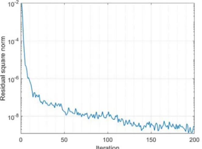
Figure 10 shows the residual evolution with the iteration number, a level of convergence under 10 dB is achieved. With the solution obtained in this step, the far-field pattern is evaluated and compared with the one obtained with the traditional planar near-field to far-field transformation (see Figure 11). The results have been depicted in the valid region of the planar transformation (~60°). The difference between the two is below -50 dB, which can be attributed to the plane truncation error introduced by the FFT windowing in the PWS transformation that is not present when using an equation system approach.

Evolution of the residual for the measurement example

Comparison of the transformed far-field using the proposed algorithm and the clasical planar

transformation.

V. CONCLUSION

A near-field to far-field transformation algorithm suited for arbitrary measurement surfaces is presented and validated using simulated and measured data. The algorithm is based on the modeling of the antenna using multiple spherical wave expansions distributed over the antenna surface. The coefficients of each spherical wave expansion are found setting up a system of equations. To accelerate the solution of the system, an iterative inversion algorithm is implemented where the matrix-vector products are replaced by fast operator using multilevel aggregation and interpolation. Simulation and measurement results show small transformation errors (50 dB) and significant computational gains.

ACKNOWLEDGEMENT

Authors would like to acknowledge Universidad Politécnica de Madrid, the Spanish Government, Ministry of Economy, National Program of Research, Development and Innovation for the support of this publication in the projects ENABLING-5G (TEC2014-55735-C3-1-R) and FUTURE-RADIO (TEC2017-85529-C3-1-R) and Madrid Region Government for the project S2013/ICE-3000 (SPADERADAR-CM).

REFERENCES

[1] O. Breinbjerg, "Spherical near-field antenna measurements-the most accurate antenna measurement technique", IEEE International Symposium on Antennas and Propagation, Puerto Rico, pp. 1019-1020, June 2016.

[2] J. E. Hansen, Spherical Near-Field Antenna Measurements. London, U.K.: Peter Peregrinus, 1988.

[3] M. A. Qureshi, C. H. Schmidt and T. F. Eibert, "Efficient Near-Field Far-Field Transformation for Nonredundant Sampling Representation on Arbitrary Surfaces in Near-Field Antenna Measurements," in IEEE Transactions on Antennas and Propagation, vol. 61, no. 4, pp. 2025-2033, April 2013.

[4] M. Farouq, M. Serhir and D. Picard, "Antenna Far-Field Assessment From Near-Field Measured Over Arbitrary Surfaces," in IEEE Transactions on Antennas and Propagation, vol. 64, no. 12, pp. 5122-5130, Dec. 2016.

[5] T. K. Sarkar, A. Taaghol, "Near-field to near/far-field transformation for arbitrary near-field geometry utilizing an equivalent electric current and MoM", IEEE Trans. Antennas Propag., vol. 47, no. 3, pp. 566-573, Mar. 1999.

[6] J. Song, Cai-Cheng Lu and Weng Cho Chew, "Multilevel fast multipole algorithm for electromagnetic scattering by large complex objects," in IEEE Transactions on Antennas and Propagation, vol. 45, no. 10, pp. 1488-1493, Oct 1997.

[7] A. Boag, "A fast physical optics (FPO) algorithm for high frequency scattering," in IEEE Transactions on Antennas and Propagation, vol. 52, no. 1, pp. 197-204, Jan. 2004.

[8] Y. Brick, A. Boag, "Multilevel nonuniform grid algorithm for acceleration of integral equation-based solvers for acoustic scattering", IEEE Trans. Ultrason. Ferroelect. Freq. Control, vol. 57, no. 1, pp. 262-273, Jan. 2010.

[9] Y. Saad, Iterative Methods for Sparse Linear Systems, 2nd edition, Society for Industrial and Applied Mathematics, 2003. [10] F. R. Varela, J. L. Besada Sanmartín and B. G. Iragüen, "Study of PO

analytic methods for serrated CATR quiet zone simulation," AMTA 2016 Proceedings, Austin, TX, USA, 2016, pp. 1-6.