1 23
Journal of Mathematical Modelling
and Algorithms in Operations
Research
ISSN 2214-2487
Volume 12
Number 3
J Math Model Algor (2013) 12:277-290
DOI 10.1007/s10852-013-9216-x
Networks-CMMSE
1 23
Data Mining with Enhanced Neural Networks-CMMSE
Ana Martínez Blanco·Angel Castellanos Peñuela· Luis Fernando de Mingo López·Arcadio Sotto
Received: 15 August 2012 / Accepted: 25 January 2013 / Published online: 28 February 2013 © Springer Science+Business Media Dordrecht 2013
Abstract This paper presents a new method to extract knowledge from existing
data sets, that is, to extract symbolic rules using the weights of an Artificial Neural Network. The method has been applied to a neural network with special architecture named Enhanced Neural Network (ENN). This architecture improves the results that have been obtained with multilayer perceptron (MLP). The relationship among the knowledge stored in the weights, the performance of the network and the new implemented algorithm to acquire rules from the weights is explained. The method itself gives a model to follow in the knowledge acquisition with ENN.
Keywords Artificial neural networks·Rule extraction· Symbolic rules·Data mining
Mathematics Subject Classifications (2010) 68Q32·62M45·62J05
A. Martínez Blanco·A. Castellanos Peñuela Basic Sciences Applied to Forestry Engineering, Technical University of Madrid (UPM), Av. Ramiro de Maeztu s/n, 28040 Madrid, Spain
A. Martínez Blanco e-mail: [email protected]
A. Castellanos Peñuela
e-mail: [email protected]
L. F. de Mingo López (
B
)Organization and Information Structure, Technical University of Madrid (UPM), Crta. de Valencia km. 7, 28031 Madrid, Spain e-mail: [email protected]
A. Sotto
Chemical and Environmental Technology, ESCET Universidad Rey Juan Carlos,
1 Introduction
The main problem that Expert Systems (ES) have is produced by the knowledge acquisition. In order to build ES and to avoid the bottle-neck in the knowledge acqui-sition process, automated learning algorithms can be used, these ones will learn from the examples that are presented. Among the methods that use learning algorithms are Neural networks (NNs). So NNs are being applied to the ES technology due to the advantages that the learning algorithms have [2,4]. NN can be useful for the knowledge base design [1,6].
However, one of the disadvantages of NN is the way of interpreting the concepts learned is very difficult [7]. This is due because neural networks have stored the knowledge in the weights linked to the connections, and therefore, it is difficult to explain the concepts in the weights from which neural networks elaborate the correct output. That is the reason Artificial Intelligence is performing some research about symbolic knowledge acquisition from a neural network [8,12,14]. Obtained rules of the neural network could give to knowledge engineering new points of view about the domain and new rules to interpret.
This work presents a new method to solve the nowadays problems about the sym-bolic knowledge acquisition from the weights of a NN. The former corresponds to the framework whose idea is to support knowledge acquisition, where the optimum way of training the network is related with the knowledge that can be acquired. The relationship among the knowledge stored in the weights, the performance of the network and the new implemented algorithm to acquire rules from the weights is explained.
The prediction volume of wood is presented as an application example, where the whole method is implemented. The presented model has been successfully applied and it is a tool that can be added to the processing and control methods available. The method itself gives a model to follow in the knowledge acquisition with NN.
2 Enhanced Neural Networks
In this work we have used Enhanced Neural Networks. The application of Enhanced Neural Networks (ENN) [10], when dealing with classification problems, is more powerful than classical Multilayer Perceptron. These enhanced networks are able to approximate any function f(x)using n-degree polynomial defined by the weights in the connections. Multilayer Perceptron MLP is based on the fact that the addition of hidden layers increases the performance of the Perceptron.
Data sets with a no linear separation can be divided by the neural network and a more complex geometric interpolation can be achieved, provided that the activation function of the hidden units is not a linear one.
networks share the inputs. Mathematically, the previous idea could be expressed as wji=ok, beingwji a weight of the main network and okthe output of a neuron in
the assistant network. Such idea permits to introduce quadratic terms in the output equations of the network where they were lineal equations using Backpropagation Neural Networks BPNN with linear activation functions. As example we considered the Eq.2of a network ENN 2–1 with an assistant network 2–3 (see Fig.1).
The weight matrix of the assistant network is given by
W = ⎛ ⎜ ⎜ ⎜ ⎝
w11 w12· · ·w1m
w21 w22· · ·w2m
... ... ... ... wn1 w22· · ·wnm
⎞ ⎟ ⎟ ⎟
⎠ (1)
The output of the main network has been defined by z(x,y)in Eq.2z(x,y)= w1x+w2y+b ,w1=w11x+w21y+b1,w2=w12x+w22y+b2, b=w13x+w23y+ b3then:
z(x,y)=w1x+w2y+b
=(w11x+w21y+b1)∗x+w12x+(w22y+b2)y+w13x+w23y+b3 =w11x2+w22y2+(w21+w12)xy+(b1+w13)x+(b2+w23)y+b3 (2) The degree of Eq.2is higher than the degree of Perceptron that is 1. In this way it is possible approximate some non lineal function without lineal separation, where Perceptron cannot do it.
If there are not hidden layers then the degree of the polynomial is two, which is a quadratic polynomial in the output of the network. The feature of being able to increase the degree of the polynomial output, adding more hidden layers, makes this kind of neural network a powerful tool against the MLP neural networks. A function could be approximated with a certain error, previously fixed, using a polynomial of n-degree P(x). The achieved error using this polynomial is bound by a mathematical expression. Then you only have to compute the successive derivates of f(x)until a certain degree and to generate the polynomial P(x).
-1
w1
w2
b
x
y
z
w11
w12
x
y
w1
w2
b
w13 w21
w23
w22 -1
b3 b2
b1
We have studied the knowledge extraction algorithms applied to a network with n inputs. Once trained the ENN, it is necessary to study the weight matrix of the assistant network in which the weights have been fixed and that provides the weights of the main network. Knowledge of the ENN is fixed at the matrix of weights of the assistant network. These weights are the ones we have applied our knowledge extraction algorithms, which are presented in the following sections. In order to interpret these weights applied to each ith column of the weights of the assistant network, it has been defined a valuewkthat is named as the associate weight to the
k-th input of main network, see Eq.3.
Let W= {wpq}the weights of the assistant network, then∀k=1· · ·q−1
wk=
p i=1
wik+wkq
, wq=wpq (3)
2.1 Polynomial Regression
This section shows an example of 2-degree polynomial regression using an ENN with no hidden layers.
Let f(x,y)a polynomial to approximate: f(x,y)=(Ax+By+C)2
= A2x2+B2y2+C2+2ACx+2BCy+2ABxy (4)
According to theoretical results the following matrix must be obtained using an ENN.
⎛ ⎝A
2 i 1 j1 i2 B2 k1 j2 k2 C2
⎞
⎠, where i1+i2=2AB,−j1− j2=2AC,−k1−k2=2BC (5)
A neural network has been trained using a random data set with an uniform distribution and describing the polynomial function:
f(x,y)= ⎡ ⎣x y1
⎛
⎝−00..660395668805
−0.1037416
⎞ ⎠ ⎤ ⎦
2
(6)
Mean squared error of the network must be equal to0, according to the theo-retical results. Next listing shows obtained results with the proposed neural network architecture. Note that MSE in the training and cross validation data sets is really low (near0).
Number of variables: 2
Coefficients (A, B, C): 0.68805 -0.6603956 -0.1037416
Squared coefficients (A*A, B*B, C*C): 0.4734127 0.4361223 0.01076232
# patterns: 2000 , Iterations: 102 , Learning rate: 0.05 , Cross val.: 20 % Mean Squared Error (TRAINING):
Standard deviation 6.048446e-14 , Variance 3.65837e-27
Min. 1st Qu. Median Mean 3rd Qu. Max.
-1.952e-13 -2.955e-14 1.502e-14 1.129e-14 5.949e-14 1.082e-13 Mean Squared Error (CROSS VALIDATION):
Standard deviation 6.181435e-14 , Variance 3.821013e-27
-1.805e-13 -2.674e-14 1.735e-14 1.186e-14 6.221e-14 1.064e-13 MATRIX Network coefficients:
[,1] [,2] [,3]
[1,] 0.4734127 -0.3912136 0.04101917 [2,] -0.5175567 0.4361223 0.15181956 [3,] 0.1017396 -0.2888405 0.01076232
A*A = 0.4734127 , B*B = 0.4361223 , C*C = 0.01076232 2*A*B = -0.9087703 , 2*A*C = -0.1427588 , 2*B*C = 0.137021
Coefficients of regression polynomial can be obtained using the weights matrix of trained neural network. Previous matrix shows final weights with a cuasi-null MSE, in our case the coefficients are the following ones (according to Eq.5):
(A2,B2,C2)=(0.4734127,0.4361223,0.01076232) (7) (2AB,2AC,2BC)=(−0.9087703,−0.1427588,0.137021) (8)
Such results are totally coherent with Eq.6, that is, proposed neural network is able to approximate the data set and generate the polynomial function that describes the data set.
Next listing shows results obtained with more than2input variables. Note that the ENN is able to approximate the data set with a null error.
Number of variables: 3
# patterns: 1200 , Iterations: 20 % , Learning rate: 0.05 , Cross validation set: 20 % Real coefficients: -0.251 0.033 -0.314 -0.805
Squared Real coefficients: 0.063 0.001 0.099 0.648
Mean Squared Error (TRAINING): Standard deviation 0.007364928 , Variance 5.424216e-05
Min. 1st Qu. Median Mean 3rd Qu. Max. -0.0145600 -0.0064310 -0.0012810 -0.0008741 0.0039250 0.0233700 Mean Squared Error (CROSS VALIDATION): Stan ard deviation 0.007403743 , Variance 5.48154e-05 Min. 1st Qu. Median Mean 3rd Qu. Max. -0.0144700 -0.0063460 -0.0009139 -0.0008817 0.0034980 0.0264900 Network coefficients: 0.078 0.017 0.11 0.634
Number of variables: 5
# patterns: 2000 , Iterations: 20 , Learning rate: 0.05 , Cross validation set: 20 % Real coefficients: 0.711 0.431 0.458 0.857 0.409 0.323
Squared Real coefficients: 0.505 0.186 0.21 0.734 0.167 0.104
Mean Squared Error (TRAINING): Standard deviation 0.0008561259 , Variance 7.329515e-07
Min. 1st Qu. Median Mean 3rd Qu. Max. -3.095e-03 -5.235e-04 1.241e-04 6.914e-05 7.022e-04 2.046e-03 Mean Squared Error (CROSS VALIDATION): Stan ard deviation 0.0009080438 , Variance 8.245436e-07 Min. 1st Qu. Median Mean 3rd Qu. Max. -2.678e-03 -5.045e-04 1.464e-04 7.691e-05 7.481e-04 1.976e-03 Network coefficients: 0.503 0.185 0.208 0.733 0.166 0.107
Number of variables: 7
# patterns: 2800 , Iterations: 20 , Learning rate: 0.05 , Cross validation set: 20 % Real coefficients: 0.129 0.398 0.444 0.345 -0.432 0.912 0.227 -0.685
Squared Real coefficients: 0.017 0.159 0.197 0.119 0.186 0.831 0.052 0.469
Mean Squared Error (TRAINING): Standard deviation 0.0006614979 , Variance 4.375794e-07
Min. 1st Qu. Median Mean 3rd Qu. Max. -1.801e-03 -5.538e-04 -1.119e-04 -8.575e-05 3.398e-04 2.196e-03 Mean Squared Error (CROSS VALIDATION): Stan ard deviation 0.0006642028 , Variance 4.411654e-07 Min. 1st Qu. Median Mean 3rd Qu. Max. -1.614e-03 -5.361e-04 -1.186e-04 -9.047e-05 3.024e-04 2.229e-03 Network coefficients: 0.018 0.16 0.198 0.12 0.187 0.832 0.053 0.466
Number of variables: 9
# patterns: 3600 , Iterations: 20 , Learning rate: 0.05 , Cross validation set: 20 % Real coefficients: -0.329 -0.717 0.765 0.126 -0.025 -0.917 0.899 0.724 -0.263 -0.667 Squared Real coefficients: 0.108 0.514 0.585 0.016 0.001 0.841 0.809 0.524 0.069 0.445 Mean Squared Error (TRAINING): Standard deviation 0.0002464544 , Variance 6.073979e-08
Min. 1st Qu. Median Mean 3rd Qu. Max. -6.969e-04 -2.121e-04 -3.974e-05 -3.869e-05 1.235e-04 8.826e-04 Mean Squared Error (CROSS VALIDATION): Stan ard deviation 0.0002595937 , Variance 6.738888e-08 Min. 1st Qu. Median Mean 3rd Qu. Max. -7.053e-04 -2.128e-04 -6.166e-05 -3.831e-05 1.235e-04 8.826e-04 Network coefficients: 0.108 0.514 0.586 0.016 0.001 0.841 0.809 0.524 0.07 0.444
Number of variables: 11
# patterns: 4400 , Iterations: 20 , Learning rate: 0.05 , Cross validation set: 20 % Real coefficients: -0.553 0.423 -0.585 0.525 -0.156 0.098 0.906 -0.943 -0.867 0.835 0.459 0.049 Squared Real coefficients: 0.305 0.179 0.343 0.276 0.024 0.01 0.82 0.89 0.752 0.697 0.211 0.002 Mean Squared Error (TRAINING): Standard deviation 2.250265e-05 , Variance 5.063691e-10
Min. 1st Qu. Median Mean 3rd Qu. Max. -7.489e-05 -1.916e-05 -4.108e-06 -3.332e-06 1.171e-05 8.005e-05 Mean Squared Error (CROSS VALIDATION): Stan ard deviation 2.36987e-05 , Variance 5.616285e-10 Min. 1st Qu. Median Mean 3rd Qu. Max. -6.592e-05 -1.746e-05 -2.043e-06 -1.089e-06 1.424e-05 7.249e-05 Network coefficients: 0.305 0.179 0.343 0.276 0.024 0.01 0.82 0.89 0.752 0.697 0.211 0.002 Number of variables: 13
# patterns: 5200 , Iterations: 20 , Learning rate: 0.05 , Cross validation set: 20 %
Real coefficients: -0.756 0.592 -0.554 -0.364 -0.28 -0.703 -0.837 0.53 -0.633 -0.739 -0.099 0.29 0.642 -0.218 Squared Real coefficients: 0.571 0.351 0.306 0.133 0.079 0.494 0.701 0.281 0.401 0.545 0.01 0.084 0.413 0.047 Mean Squared Error (TRAINING): Standard deviation 1.333839e-05 , Variance 1.779126e-10
Fig. 2 Different shapes obtained using ENN with no hidden layers, corresponding to XOR, circle, ellipse and parabola functions. MSE is near to0.0with100iterations
Such results show in a practical way the universal approximation property of ENN [10,11] (Fig.2).
3 Material and Methods
rate for each trained ENN [3]. A second part, when you are training an ENN, it is possible to know the effect, each one input is having on the network output. This provides feedback as to which input channels are the most significant. From there, you may decide to prune the input space by removing the insignificant channels. This will reduce the size of the network, which in turn reduces the complexity and the training times and error [9].
One last stage of processing of rules that identified the behavior of the input variables (antecedent of the rule) in each output classes (consequents of rules). Finally, when the rules have been established. Therefore there will be achieved a control system. The model presented has been successfully applied to the prediction volume of wood. ENNs are thus a useful and very powerful set of tools that can add to the large number of processing and control methods available.
First Step: the first stage, this method obtains the consequents or the output in a rule. First of all, it is necessary a normalization of initial set of training patterns, input and output variables in the interval[−1,1]. This standardized set of patterns is ordered from the smallest to the biggest output. The first option was to divide the whole range[−1,1]in k output intervals with the same number of patterns in each interval.
A second option was proposed, the output is divided into intervals k units wide, obtaining K2 training subsets from each output interval I1· · ·I2
k , where Ii=
[−1,−1+k)· · ·I2
k =(1−k,1]and k=1+3.322 log10n [13] and n is the number of
patterns. Those intervals will be the consequents of the extracted rules.
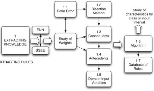
Finally we developed a new method, named Bisection Method (BM), which was provided a better error rate in the training of each interval than the other methods named, and it is discussed below. Figure3shows a summary of the whole process.
1 EXTRACTING KNOWLEDGE
Study of Weights
1.1 Ratio Error
1.2 Bisection
Method
1.3 Consequents
1.4 Antecedents
1.5 Domain Input
Variables ENN
SSEE
EXTRACTING RULES
1.6 Algorithm
1.7 Database of
Rules Study of characteristics by
class or input interval
3.1 First Step: Bisection Method (BM)
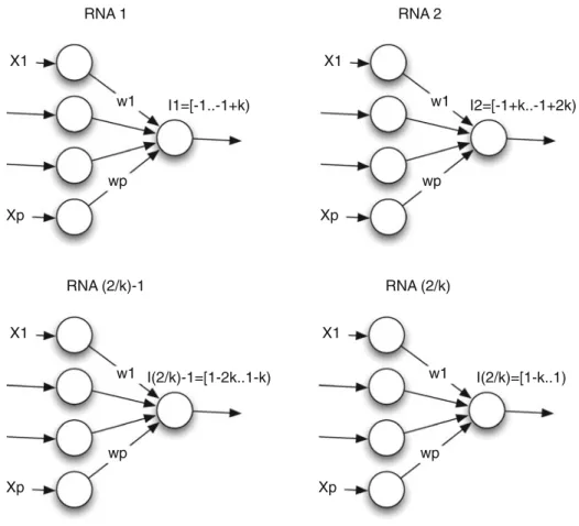
Once the set of patterns has been sorted, the output is divided in two intervals, and iteratively division is performed. A first division of the values associated to the output variable, in two intervals: positive output (0,1] and negative output[−1,0). Two independent neural networks are defined in order to be trained. Each one neural network is trained with n inputs and only one output. Each one of the two output intervals is divided in two new classes. This division is performed iteratively, studying the variation of weights. When in a new division the weights do not change, then go back to the initial division, and finish the division of the sets of patterns. A division of the set of training patterns is made according to their outputs, the output range is divided into intervals, for each output interval Ii, a set of training Si is considered,
an independent neural network is trained, as it is shown in Fig.4. The initial pattern set is classified in several subsets and therefore into several ENNs. When output intervals are fixed, the consequents of the rules have been fixed by BM.
Obtaining consequent rules or output intervals Iifor a prediction function:
1. Standardization of all patterns in the interval[−1,1]. 2. Order the set of patterns from low to high output.
X1
Xp
w1
wp
I1=[-1..-1+k) RNA 1
X1
Xp
w1
wp
I2=[-1+k..-1+2k) RNA 2
X1
Xp
w1
wp
I(2/k)-1=[1-2k..1-k) RNA (2/k)-1
X1
Xp
w1
wp
I(2/k)=[1-k..1) RNA (2/k)
3. Divide the ordered set of patterns S in n subsets S1∪ · · · ∪Sn, with Si∩Sj= ∅
and∪Si=S and∪Ii= [−1,1]by (BM) in the previous step and so that in each
subset Si all output values have the same sign. Building one ENNitrained with
each Si. The range Ii determines the consequents rules that are extracted from
each ENNi.
3.2 Second Step: Algorithm to Extract Predictive Variables (EM)
Now, the importance of each input variable must be studied for each different training network ENNi, taking into account the weights in each one, and so we must
repeat the next algorithm for each one ENNiobtained in the first step. In this process,
antecedents should be chosen in order from biggest to smallest absolute value of the weights of the connections of input variables, in such way, that each variable antecedent verifies:
wijujCk>0 (9)
where Ck= {−1,1} is the kind of inference, negative or positive (where i is the
number of the outputs interval).
It can be studied in which range of allowed values of the input variable, along with the other variables that contribute to the output, is possible to obtain the whole output range which is being studied. The range of the variables antecedents would never be the whole interval[−1,1], due to the sign of the weights will determine if the variable will be positive or negative according to Eq.9.
To determine the best set of forecasting variables, in each subset of training Si
with output in Ii:
– Analyze the variation of the values of the input variables for each training subsets Si, in each ENNicalculating the interval(μij−σij, μij+σâ ˘A ¸Sij)for each variable
μjin Ii.
– For each ENNibuilt in step 1, extract important input variables or antecedents,
from it following next steps:
1. CURRENT=wi0(bias term)
UNKNOWN=uj∈UNUSEDVARS|wij|
2. Stop if exist values for uj∈ [−1,1]such
wi0+uj∈USEDVARSwijuj− f
−1(z
i) >UNKNOWN
zi∈Ii,zi=min{Ii}
Where ai· · ·aj are input values of the variables ui· · ·uj and ui· · ·uj∈
USEDVARS.
If you want get more input variables for the output class Ii (consequent
selected) go to step 3.
3. Choose a new variable uk∈UNUSEDVARS such|Wik|is the maximum
value and where Ciwik≥0. It gets a new antecedent of the rule.
4. CURRENT=CURRENT+Wik
UNKNOWN=UNKOWN− |Wlk|
UNUSEDVARS=UNUSEDVARS−(uk)
3.3 Third Step: Obtaining Rules
In the previous step, the antecedents of the rules have been obtained, this is the most influential input variables for each output interval Ij, each trained ENNj.
When the rule Rjhas been formulated, the most important condition has been
given for output in a given interval[−b,−c). The rule obtained is that the weights are provided, as the most important feature of this interval. Ifμui[−b,−c)andσui[−b,−c)
are the mean and standard deviation of variable ui in the output range[−b,−c).
Then we take as domain and therefore antecedent for this interval, the values that the variable uitakes on interval.
Thus, we obtain as the first major rule or rule over the output interval[−b,−c) If ai∈→output∈ [−b,−c)=Ij (10)
Or which is the same: If ai∈→Ij.
Where i is the number of the input variables and j is the number of output intervals. In this way we are indicating that in the output range Ij, the most important
variable is the i-th input variable and we are giving the values taken by the i-th input variable for the output set Ij. Finally, the knowledge extraction for every net ENNj
is made, obtaining a rule or a subset of rules for each output interval. Each rule Rjcorresponds to an output interval. Each output interval has an associated ENNj,
the network has been trained and whose weights define the variables that must be antecedents of each rule. We enunciate more general rules with one antecedent or finer rules with more than a single antecedent.
Rk:If μi∈ [a,b)∧ · · · ∧μj∈ [c,d) then Ik (11)
If the rule is verified for the extreme values of the interval, you will be checking for the rest of the values within the range of variation of the antecedent.
4 Data Mining Using Enhanced Neural Networks
We have studied the behavior of the weights of the network, for a first data set defining a function exactly. It is a collection of values that define a functional relationship (deterministic). If the network is trained in which the input patterns are the independent variables in the functional relationship and the output pattern of the network is the dependent variable y. The network learns the relationship among the variables and the values which constitute the dependent variable are predicted by ENN. We have studied this case, to check the level of knowledge stored in the weights. The relationship between the independent variable and the dependent variable is shown in the values of the weights, some examples are explained below. A table of values for independent variables and the corresponding values for the dependent variable is performed. With these data the network is trained.
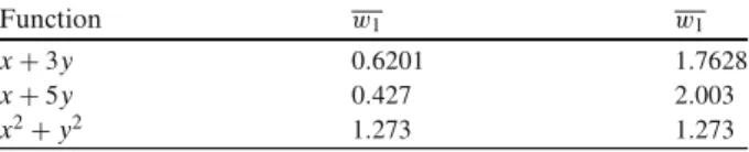
Table 1 Weights associated in
different training functions Function w1 w1
x+3y 0.6201 1.7628
x+5y 0.427 2.003
Table 2 Weights associated function f(x,y)=x+y2over different input range (an implementation in R has been used)
Domain input w1 w1 Mean squared
variables error
[0,100) 0.0121 1.3807 0.101
[1,100] 0.0413 1.6128 0.003
[0,1] 0.6175 0.6431 0.002
[1,2] 9.838 27.027 0.030
[0.5,1] 2.776 0.274 0.002
Table1shows as the value of the weights preserves the relationship between the independent variables, the weight of the variable y is three times that of the variable x in the first case and in the second case is actually five times the weight of the variable x. The weight value of the variable y, in both cases the variable with the most influential is the variable y, with different degrees in each case. The importance of the input variables is reflected in the weights. In the third case, not working with a linear function, but this is a case in which the behavior of the variables is symmetrical, both variables influence in the same way in the output value; with different ENNs have been obtained similar weights. This study has confirmed that the knowledge of the network, once trained, is stored in the weights.
We have studied the function f(x,y)=x+y2 and we have generated random patterns for the variables x and y, then we have observed the behavior of the weights changes according to the range of input values. So if we work with values obtained at random in the interval[1,100]for the input variables x and y the weights obtained have different characteristics that if we work with values for input variables in the interval [0,1]. It seems clear just, when a variable takes values in it [0,1] and is squared, the value of the variable will decrease, as in this way is described by the values of the weights for the variable y. However, if the variable takes values greater than1then the variable is greater than being squared. Both features for the same function are reflected in the weights of the trained networks for different range of the input variable y (see Table2).
All results show that the importance of the input variables change when the range of input variables change. Yet it is confirmed that the proposed method depends on: – First step: divide the set of patterns for its outputs and the study of interrelation-ships between the input and output variables. Sometimes, the variation in the range of the output variable causes changes on the importance of input variables and then it is necessary to divide the range of the output variable in class, for a separate study of each output class.
– Second step: study the range and weights of the input variables in each range of the output variable obtained in the previous step.
– Third step: extract rules using steps one and two.
5 Example of Application
of wood for a given area or forests and for a given tree species in different natural environments. The data set file [5] has been used in order to implement method explained in the Section3. The example of application is a dataset from eucalyptus obtained from a region in Spain. The main aim is to detect relationships between all the variables that are in our study, and also this work seeks to estimate the wood volume. The input variables considered for the network were diameter, thickness bark (crust); grow of diameter, height and age. The output variable was the volume of wood.
The Enhanced ENNs were trained, but in any case learning didnt improve, initially tested the whole set. The ratio of error should not be acceptable; the knowledge learned by the network is not good, the error is too large. The evolutions of the values of the weights, in different division intervals for all patterns, the first division in positives and negatives outputs in, finally four networks have been trained. The error is less when the total pattern set is divided in subsets and one ENN is trained for each subset of pattern. In this example, finally 4 neural networks were constructed: one for each set of patterns S1· · ·S4 obtained, which outputs are I1· · ·I4, .One neural network is trained for each interval. Now, in each one of the sets of patterns obtained, the most important input variables, in each one of the subsets is sought, using the algorithm for extraction (EM). Table 3 shows the weights of the four trained networks obtained in the first phase BM.
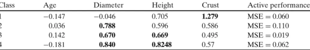
In the second step, the method named as EM has been implemented. Now when the set is divided into four subsets and the weights are observed in each obtained subset or class, it is possible to detect that the most important input variable is changing in each class, by the weights in each neural network. The crust appears as the most important variable followed by height in the first class, in the class two the most important input variable has changed and now the principal variable is the diameter and in the third class the same importance for diameter and height and in the fourth class is the diameter the most important variable again. Weights are studied when they are stable and do not change.
Table4shows the possible domain of antecedents of the rules. In the third step the solution is a set of rules. Using sections 3.2 and 3.3, the following rules have been obtained from the nets. To apply the rules extracted above to the studied case about volume of wood. The rules show that the network has learned, and then it is possible get a good set of rules if there was a good learning ratio in the training network. For each output interval a set of rules is obtained with one or more variables as antecedents, so the rules are obtained:
if crust∈ [4,13.6] ∩height∈ [9.5,14.2] →volume∈ [22,64]
Table 3 The most important input variables: weights associated over each output interval volume (or class) with the mean square error (MSE) obtained by ENN
Class Age Diameter Height Crust Active performance
1 −0.147 −0.046 0.705 1.279 MSE=0.060
2 0.036 0.788 0.596 0.586 MSE=0.110
3 0.142 0.670 0.669 0.495 MSE=0.019
Table 4 Values of the variables in each ENNi
Class Volume Diameter Crust Height Age
Average 1 43.39 9.55 8.84 11.9 12.9
Deviation 1 20.7 2.06 4.76 2.32 4.54
Average 2 95.13 13.13 17.4 16.41 12.9
Deviation 2 12.55 1.16 5.16 1.62 4.44
Average 3 161.33 15.61 26.087 19.48 1.4
Deviation 3 25.24 1.27 5.66 2.03 3.38
Average 4 476.87 22.89 69.3 25.88 15.43
Deviation 4 226.21 4.19 30.1 4.33 2.53
Domain antecedents of rules
if diameter∈ [12,14.3] ∩height∈ [12.4,22.5] →volume∈ [82,107]
if diameter∈ [14.3,16.9] ∩height∈ [20.4,31.7] →volume∈ [136,186]
if diameter∈ [18.2,27] ∩height∈ [39,99] →volume∈ [250,703]
if diameter≥14.3∩height≥20.4→volume≥136
if diameter≥14.3∩crust≥40→volume≥136
The problem under study is prediction of volume of wood, and the rules obtained are useful in order to estimate the amount of wood using typical tree variables and the Knowledge obtained is compared with other methods such as repository and with the tree volume tables for a given tree species and for prediction methods as regression. The results are similar in each case.
6 Conclusions and Final Remarks
A new method to extract rules from a neural net has been elaborated. In this way the rules obtained will allow completing the knowledge that could be extracted from an expert when building the knowledge base for an ES. In the proposed method, a model of ENN has been used. The implemented method is effective when the importance or characteristics of forecasting variables could change depending on the range of forecast variable.
can be updated and improved the database, more easily and can go to expand the database of rules obtained.
References
1. Andrews, R., Geva, S.: Rule extraction from local cluster neural nets. Neural Comput. 47, 1–20 (2002)
2. Boger, Z., Guterman, H.: Knowledge extraction from artificial neural networks models. In: Proc. IEEE Int. Conf. Systems, Man and Cybernetics, pp. 3030–3035. IEEE Press, Orlando (1997) 3. Castellanos, A., Castellanos, J., Manrique, D., Martinez, A.: A new approach for extracting rules
from a trained neural network. Lect. Notes Comput. Sci. 1323, 297–302 (1997)
4. Heh, J., Chen, J.C.: Designing a decompositional rule extraction algorithm for neural networks with bound decomposition tree. Neural Comput. Appl. 17(3), 297–309 (2008)
5.http://acer.forestales.upm.es/basicas/udmatematicas/matematicas1/datos/Eucaliptos.pdf (2011). Accessed 15 Aug 2012
6. Kamruzzaman, S.M., Jehad Sarkar, A.M.: A new data mining scheme using neural networks. Sensors 11, 4622–4647 (1997)
7. Kolman, E., Margaliot, M.: Are artificial neural networks white boxes? IEEE Trans. Neural Netw. 16, 844–852 (2005)
8. Malone, J.A., Mcgarry, K.J., Bowerman, C.: Rule extraction from Kohonen neural networks. Neural Comput. Appl. 15, 9–17 (2008)
9. Martinez, A., Castellanos, A., Hernandez, C., Mingo, F.: Study of weight importance in NN. Lect. Notes Comput. Sci. 1611,101–110 (2004)
10. Mingo, L.F., Martinez, A., Gimenez, V., Castellanos, J.: Parametric bivariate surfaces with neural networks. Mach. Graph. Vis. 9(2), 41–46 (2002)
11. Mingo, L.F., Ablameyko, S., Aslanyan, L., Castellanos, J.: Enhanced Neural Networks with Time-Delay in Trade Sector, Digital Information Processing and Control in Extreme Situations, pp. 202–208. Belarus Academy of Sicence, Minsk (2002)
12. Setiono, R., Kheng, W., Zurada, J.: Extraccion of rules from neural networks for nonlinear regression. IEEE Trans. Neural Netw. 13(3), 564–577 (2002)
13. Sturges, H.A.: The choice of a class interval. J. Am. Stat. Assoc. 21(153), 65–66 (1926)