Transportation Research Procedia 14 ( 2016 ) 2870 – 2879
2352-1465 © 2016 The Authors. Published by Elsevier B.V. This is an open access article under the CC BY-NC-ND license (http://creativecommons.org/licenses/by-nc-nd/4.0/).
Peer-review under responsibility of Road and Bridge Research Institute (IBDiM) doi: 10.1016/j.trpro.2016.05.404
ScienceDirect
6th Transport Research Arena April 18-21, 2016
The impact of the structure of the economy on the evolution of road
freight transport: a macro analysis from an Input-Output approach
Ana Alises
a,*,
José Manuel Vassallo
aaTransport Research Centre (TRANSYT). Universidad Politécnica de Madrid. Avda. Profesor Aranguren s/n. – 28040 Madrid (Spain)
Abstract
Understanding the link between transport and the economy has been of the greatest concern among researchers and practitioners. This research explores the impact of the economic restructuring processes in the aggregate road freight transport demand. We develop a simulation exercise of two alternative economic scenarios over the period 1999–2011 in Spain and the UK by means of an extended Input-Output model. This approach allows us to calculate the elasticity range of vehicles-km to GDP depending upon the types of economic activity developed in these countries and their dematerialization level. The results confirm that the transition to more service-oriented economies implies much lower transport requirements, as has been the case in the UK. Furthermore, the comparison of the two countries has contributed to highlight the importance of other set of non-economic variables, related to technological, logistics and modal factors in the definition of final road freight transport demand.
© 2016The Authors. Published by Elsevier B.V..
Peer-review under responsibility of Road and Bridge Research Institute (IBDiM).
Keywords: GDP structure; dematerialization; road freight traffic; Input-Output
* Corresponding author. Tel.: +34 679 84 54 15. E-mail address: [email protected]
© 2016 The Authors. Published by Elsevier B.V. This is an open access article under the CC BY-NC-ND license (http://creativecommons.org/licenses/by-nc-nd/4.0/).
1.Introduction
For decades researchers and practitioners have taken for granted the link between economic growth and freight transport demand. However, in several countries the historical elasticity values between transport and the economy have been radically changing over the last few years (Gilbert and Nadeau (2002) and Sorrell et al. (2012)). This fact demonstrates that the real cause-effect relationship between these two variables is not yet fully known.
A good understanding of the nature of the relationship between road transport and the economy is crucial for several reasons. First, because this relationship is supposed to help planners estimate the evolution of road freight transport demand over the years. And second, because knowing this relationship will help policy-makers adopt measures to promote sustainable growth since road traffic is responsible for a wide amount of externalities (European Union (2001), OECD (2002), OECD (2006)).
Up to now, the existing methodologies applied to explain road freight transport demand have been based on simulating the behaviour of multiple factors – including economic growth – influencing transport by using different models (e.g. Jong, Gunn. and Walker (2004) and Tavasszy (2006)). However, previous studies highlight the complexity of developing such type of models, partly because of the numerous factors determining the shipping of commodities in each country, and partly because of that lack of available data (Elaurant and Bates (2007)).
In the last few decades, there have been significant changes in the structure of the economy of many developed countries. The contribution of service-oriented sectors – such as financial services – to the national GDP has been growing in importance compared to, for instance, manufacturing activities. This trend has led to the
“dematerialization of the economies”. That means the ‘reduction of material resources required per unit of GDP’
(Schleicher-Tappeser and Steen (1998) and even though it is well known that this process results in decoupling levels between transport and the economy, little research has been conducted about the impact of dematerialization on road freight transport trends.
This research intends to measure the impact that the structure of the economy has on road freight transport demand at the macro level – using a top-down approach – in a certain geographical area. For this purpose, we use an extended Input-Output (IO) model linking both the economic structure – structural relationships of production and consumption over time – and the road transport intensity in a certain country or region.
We have developed a methodology based on the definition of two scenarios that reflect a hypothetical evolution of the structure of the economy – towards a full dematerialization or a full materialization – and applied them to two case studies: Spain and the United Kingdom (UK). This methodology enables us to compare the results of the scenarios with the actual trends in terms of goods transport demand, and obtain conclusions from them.
The paper is structured as follows. In Section 2, right after the introduction, we identify the key variables explaining road freight transport trends from a macroeconomic standpoint. In Section 3 we define the methodological approach – the model and the scenarios. In Section 4 we provide an overview of the economic and transport characteristics of each case study. In Section 5 we show and describe the results obtained from the analysis. Finally, in Section 6, we highlight the main conclusions of this research.
2.Key drivers to explain road freight transport demand
It is well known that there exist a link between transport and the economy, but this relationship is complex because economic growth is not the only factor that determines freight transport trends. Effects such as technological innovations, changes in final demand or logistic improvements may also contribute to modify transport patterns (Alises et al. (2014)).
Road freight volumes are influenced by a wide range of factors that explain different trends across countries. Transport volumes depend on the levels of national economic output and consequently on the need to ship the commodities produced among different regions; and, on the other hand, on the organization of both the supply chains and transport systems.
2.1.Using Input-Output Tables for transport modeling
The necessity of knowing the influence of changes in the production structure and economic patterns that may influence transport demand over time led to a new body of works in transport modelling. This is characterized by the development of transport IO models at urban and regional scale (see Ivanova (2014) for a deeper review).
The main reason for this trend is that several authors have pointed out the advantages of using these models in representing intersectorial interdependencies in production/consumption (Cascetta (2013)). This is crucial to define the interchange of goods – trade flows – and therefore the movement of goods in a region.
As previously said, research within this field has led to a number of operational land use-transportation models by incorporating spatial (or interregional) disaggregation data. Some examples are MEPLAN (Hunt and Echenique (1999)), TRANUS (de la Barra (1995)), PECAS (Hunt and Abraham (2003)) and RUBMIO (Kockelman et al. (2005)). These models combine IO data with additional information for trade and travel choices (travel costs, location of activities and population, mode choice models, etc.). That means that they usually need a big amount of available additional micro data to describe travel flows.
The IO approach has also been used to conduct several analysis at the macro level for planning processes and policy design in sectors such as the energy sector (see e.g. Lenzen and Foran (2001) and Alcántara and Padilla (2003)). It is noted that this type of studies has never been conducted for transportation field.
2.2.The role of road freight transport intensities in explaining transport trends
Freight transport volumes are also strongly influenced by the organization of supply chains. The transport system evolves and adapts progressively to respond to the requirements imposed by the emerging new organization of logistics systems. As Woxenius and Sjöstedt (2003) argued: logistics and transport systems are complementary.
Recent years have seen technological developments, increasing specialization, more sophisticated production processes, new distribution systems, and an ever greater concentration of manufacturing and storage (McKinnon and Woodburn, (1996)). All these factors have prompted changes in production and therefore in transport patterns, as supply chain organization influences aspects such as transport distances or modal split (OECD, (2006)). Therefore it is crucial to consider these factors as drivers of road freight volume. Previous literature found that all of these industrial, logistics and transportation systems changes can be understood through the so-called Road Freight Transport Intensity ratio (RFTI) (see e.g., McKinnon 2007, Kveiborg and Fosgerau (2007) or Piecyk and McKinnon (2010)) as a means of measuring “transport efficiency” in a certain country.
Brunel (2005) defined this ratio as the number of road freight transport units necessary to produce one dollar or one euro of GDP in a country. So, this could be measured in terms of tonne-kms per GDP, or even better veh-km per unit of GDP. However, authors such as Åhman (2004) argue that constructing sectional freight intensities based on sectors’ production – that is sectorial output – instead of GDP allows a deeper and more accurate understanding of transport growth in a certain economy.
RFTI – measured as ᦼ ሾ̈́ሿΤ – can be decomposed into several ratios whose values may change over time in terms of industrial, logistics and transportation systems restructuring (Mckinnon 2007). These ratios help explain the evolution of transport trends over the years. These ratios are:
x Average value density: weight of goods of a certain economic branch divided by the monetary production value of this branch (tonne/$). Changes in this ratio are explained by new product design techniques, manufacturing processes, and the current tendency to use lighter materials;
x Handling factor: referring to the number of times a product is lifted between the origin (production centre) and destination (consumption centre) in the supply chain for each type of commodity;
As Lehtonen pointed out in 2008, there are usually difficulties in accessing quality, reliable and complete data about both handling factors and value densities. In view of that, a new ratio can be defined:
୪୧୲ୣୢΤሺ̈́ሻǡ which is equal to the inverse value density times the handling factor. This ratio is named
“freight intensity”. It is defined as the tonnes lifted divided by the value of the total production.
x Modal split: tonnes hauled by road compared to other modes;
x Average length of haul. This value depends on the location of industrial production, storage and consumption centres, and on the characteristic of the road networks;
x Load factor: the relation between the total tonnes carried and the loaded vehicles. It depends on both the mix of vehicles (with different sizes and capacities) and the lading factor of individual vehicles;
As equation (1) shows, by multiplying these ratios we obtain the RFTI in a certain country for sector in a specific year, that is ୧.
ܴܨܶܫൌݒ݄݁ᦼ݇݉ݏܱݑݐݑݐௗǡ ሺ̈́ሻ
ൌ ݐ݊݊݁ݏ௧ௗǡ ܱݑݐݑݐሺ̈́ሻ
ᇣᇧᇧᇧᇤᇧᇧᇧᇥ
௧௧௦௧௬
ൈݐ݊݊݁ݏ௧ௗǡௗǡ ݐ݊݊݁ݏ௧ௗǡ
ᇣᇧᇧᇧᇧᇧᇤᇧᇧᇧᇧᇧᇥ
ௗ௦
ൈ ݐ݊݊݁ᦼ݇݉ݏௗǡ ݐ݊݊݁ݏ௧ௗǡௗǡ
ᇣᇧᇧᇧᇧᇧᇤᇧᇧᇧᇧᇧᇥ
௩௧௨
ൈ ݒ݄݁ᦼ݇݉ௗௗǡ ݐ݊ᦼ݇݉ௗǡ
ᇣᇧᇧᇧᇤᇧᇧᇧᇥ
௩௦ௗ௧
ൈ ݒ݄݁ᦼ݇݉ ݒ݄݁ᦼ݇݉ௗௗǡ
ᇣᇧᇧᇧᇤᇧᇧᇧᇥ
௧௬௨
(1)
3.Methodological framework
One of the contributions of our paper consists of the definition of a new methodology that uses the information provided by the Input-Output tables to explain transport trends at the country level. This approach does not require as much information as some of the previously mentioned models do. However, by using aggregated information at the country level, it allows us to explain the global road freight transport trends in a certain country.
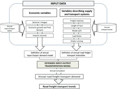
Figure 1 shows the methodological framework we use to connect economic and transportation variables – annual IO and RFTIs data – through an extended IO model. This framework will be used later on in this paper to simulate global road freight transport trends.
Fig. 1. Methodological framework scheme to estimate road freight transport demand.
The availability of IO tables for consecutive years in certain countries allows us to study the evolution of the factors previously mentioned and therefore to analyze how they influence road freight transport trends. On the other hand, countries are characterized by road freight transport intensities (RFTIs), which in their turn can be decomposed into several ratios. Annual RFTIs can be calculated as long as the information about national production and transport volumes is available. RFTIs can be explained in terms of other variables insofar as data such as modal split or length of haul is available at the national level. Below we explain our model in greater detail.
3.1.The extended Input-Output model
basic IO model establishes a balance between total supply and total demand expressed by the equation of Leontief
ൌ ሺ െ ሻିଵ, (Leontief (1936)) where is the production vector – that is, the total output corresponding to the
sectors of the economy, is the final demand vector – including both domestic demand and exports – and ሺ െ ሻିଵ is the Leontief inverse matrix ሾሿ– which reflects the requirements of any industry supplied by the rest of sectors and by itself.
The IO approach can be extended by adding complementary information to the basic IO model to overcome the limitations of the information provided by the IO tables. Our IO model follows this approach by linking a vector of road freight transport intensities to a symmetric IO table sector by sector for the same year. This modification intends to show the structural relationship between economic activities and final road transport demand in a country.
In the following equations the economy is supposed to be structured in economic sectors. Moreover,
diagonalization and transposition will be respectively denoted by ^ and ‘.
is as a vector (n x 1) that contains the road freight transport demand sorted by commodity class. The road freight transport intensity vector ( ) can be defined according to the following equation:
ܴܨܶܫ ൌ ܶԢሺݔොሻିଵ (2)
Thus, we can obtain the road transport volume T in the following way:
ܶ ൌ ܴܨܶܫ ݔ (3)
Taking the value of from the Leontief model, it leads to our extended IO model:
ܶ ൌ ܴܨܶܫ ሺܫ െ ܣሻିଵ݂ (4)
where the vector RFTI integrates transport flow data into the IO traditional analysis.
On the other hand, in an IO table the final demand can be calculated as the summation of the GDP vector – value added by sector – plus the vector containing the volumes of sectorial imports. So, the vector can be expressed by other two vectors (n x 1) that contain these components sorted by economic sector.
ܶ ൌ ܴܨܶܫ ሺܫ െ ܣሻିଵሺܩܦܲ ܫ݉ሻ=ܴܨܶܫ ܮሺܩܦܲ ܫ݉ሻ (5)
The matrix ሾሿ and the vectors used – ǡ and– in this transport model must reflect an identical disaggregation in the activity branches considered. To that end the IO data and the transport data have to be homogenized in the same number of sectors when applying this formulation.
This model has been defined to explain road freight transport volume in terms of its own economic activity and some characteristics of the transport sector. That is to say, the model measures the volume of transport that is observed in each country as a consequence of national production and consumption, imports and exports of that country according to the IO tables. However, it is important to note that this model is not able to explain all transport volumes as it does not capture cross-country traffic – that is road traffic from one neighbouring country to another neighbouring country passing through the country of analysis.
3.2.Structural decomposition analysis
The structural decomposition analysis (SDA) has been widely used in the economic literature to identify the driving factors of changes over time. All variants of SDA are static comparative methods that examine time series of sector-level and/or country-level data. In essence, SDA formulates a variable, in our case road freight traffic, in veh-km, as the sum or product of several explanatory variables. For the purpose of this research, these variables are (1) road freight transport intensities; (2) production linkages depending on the inter-sectorial relationships described by [L]; (3) sectorial GDP values; and (4) import volumes. A pair-wise comparison of changes at two specific periods of time can be undertaken by each of these explanatory variables.
explanatory variable evolves in a different way compared to the actual scenario. The SDA is conducted according to the equation (6) (Dietzenbacher and Los (1997)).
Through it, we can calculate the differences, in terms of aggregate road freight transport demand (ȟିଵ), between the base year – expressed by superscript 0 – and each one of the subsequent years in the study period –
expressed by superscript 1. This way, we can estimate the trend followed by the road freight transport demand in each country for the different hypothetic scenarios.
߂ܶିଵൌ ൬ͳ
ʹ൰ ൫߂ܴܨܶܫ ൯
ିଵ
ሾሺܮሺܩܦܲ ܫ݉ሻሻ ሺܮଵሺܩܦܲଵ ܫ݉ଵሻሻሿ
൬ͳ
ʹ൰ ൣܴܨܶܫሺ߂ܮሻିଵሺܩܦܲଵ ܫ݉ଵሻ ܴܨܶܫଵሺ߂ܮሻିଵሺܩܦܲ ܫ݉ሻ൧ ൬ͳ
ʹ൰ ൣ൫ܴܨܶܫܮ൯ ൫ܴܨܶܫଵܮଵ൯൧ሺ߂ܩܦܲሻିଵ ൬ͳʹ൰ ൣ൫ܴܨܶܫܮ൯ ൫ܴܨܶܫଵܮଵ൯൧ሺ߂ܫ݉ሻିଵ
(6)
3.3.Economic scenarios
To measure the impact of the structure of the national economy on road freight transport we have defined two hypothetical scenarios where the economy evolves in the opposite way.
x Scenario 1 (full materialization). All the GDP growth in a certain country is absorbed by transport intensive sectors: According to this scenario we suppose that service-oriented branches of the GDP no longer grow after the base year. Consequently, intensive sectors experience a higher increase in their GDP compared to the actual scenario. The growth across intensive sectors is allocated according to their weight in the GDP of the base year.
x Scenario 2 (full dematerialization). All the GDP growth in a country is absorbed by service-oriented sectors: In this case we assume that the economic growth of each country results from service-oriented sectors. Consequently transport intensive sectors no longer grow after the base year.
For each of these scenarios we keep unchanged values (throughout all the study period) of the following variables: (1) the actual the global GDP growth, (2) the road freight transport intensity changes, and (3) the sectorial linkages and the volumes of imports values. The only variable we change is the structure of the GDP. Through these scenarios we seek to examine what would have happened to road volumes if GDP structure had evolved in a opposite way.
4.Empirical application: case studies and data
In order to apply the methodology defined in the previous section, we chose two case studies: the UK and Spain. We decided to select these countries for several reasons. First, different transport trends have been observed in the UK and Spain. In Spain road transport growth has closely followed GDP growth whereas in the UK high levels of decoupling have been reported. In the case of Spain we found that one of the main reasons explaining road freight transport trends was the impact of the construction sector, which contributed to curb decoupling by increasing the tonnes lifted across the country (it increased by more than 4% between 1999 and 2007, until the arrival of the economic crisis). In contrast, in the same period, most of the growth of the UK economy was produced by service--oriented sectors – with a share of 75.51% of the GDP in 2007. Therefore, we thought that it could be interesting to study in greater detail how road freight transport would behave in these two countries under similar restructuring processes of their economies. The second reason for selecting these countries is that there is enough homogeneous data available for the two of them – from both the macroeconomic and the transportation side. The third reason is the fact that cross-country transport, which is not captured by our methodology, in the UK and Spain is negligible compared to other type of transport.
As we needed to integrate both transport and economic data in our methodology, we had to homogenize the information from the two databases. To that end, the original IO tables were aggregated into eight sectors representing the main areas of economic activity. This aggregation was made according to the commodity groups of the transport dataset. Transport data series from EUROSTAT changed its classification in 2007, so we have to homogenize the series across all the years of the period of study. Finally, we consider the following groups: (1) food, beverage and tobacco, (2) mining and construction, (3) textile sector, (4) energy: fuel and power products, (5) chemical products, (6) machinery and transport equipment, (7) manufacturing products and (8) services. The first seven sectors include the eighteen transport-intensive industries from the IO tables.
It is noted that the statistical data on transport by commodity class in a country provided by the EUROSTAT database only include transport operations made by domestic hauliers. This means that the foreign hauliers’ activity is left out of the picture of this analysis. Nevertheless, in our two case studies this part of the transport volume only accounts for about 1% of the total road transport demand – between 0.6 and 0.8% in Spain and 0.9 and 1.1% in the UK according to EUROSTAT data series – so the distortion of the results is expected to be negligible.
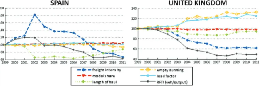
Transport data is used to calculate the RFTIs that are subsequently introduced in our IO model. As the results of our simulation exercise strongly depend on the evolution of the RFTI, this ratio deserved to be analyzed in greater detail along with other ratios. This evolution is shown in Figure 2. Table 1 contains the mean values observed during the period of analysis. All these values are calculated on the basis of the EUROSTAT data series from 1999 to 2011.
Fig. 2. Evolution of global RFTI –ݒ݄݁ᦼ݇݉ ݑݐݑݐΤ – and related ratios from 1999 to 2011 in Spain and the UK. Index 1999=100.
Looking at the graphs, several similarities and divergences between the behaviour of the key ratios in the two countries can be highlighted. The most notable case is the evolution of the amount of tonnes lifted per unit of monetary production. Whereas in the UK this ratio has been steadily decreasing ever since 1999, in Spain it significantly increased in 2002 and no lower values had been recorded after the base year until the arrival of the crisis. The mean value for this ratio is 68% higher in Spain than in the UK.
The growth of the service sector in the UK entailed fewer trips across the country. By contrast, the main reason for the trends observed in Spain was the expansion of the construction activity since mining and construction goods are low value materials and generate numerous as well as short-length trips. This fact may also explain the remarkable reduction of the average length of haul recorded in the country from 2001 and 2002.
The rest of the ratios have not changed substantially in Spain whereas in the UK both the load factor and empty running ratios have increased. Modal share has remained stable in both countries.
Table 1. Mean values of RFTI and related key ratios in Spain and the UK in the period 1999–2011. ܜܗܖܖ܍ܛ
ܗܝܜܘܝܜሾܕܑܔܔܑܗܖܛ܃܁̈́ሿ
ൗ Modal
share
Length of haul
Empty running
Load factor
RFTI
(ܞ܍ܐൗܗܝܜܘܝܜሾܕܑܔܔܑܗܛ܃܁̈́ሿ)
Spain 861.4 94.7 122.5 27.4% 15.8 7011
UK 511.5 88.8 95.0 22.1% 9.2 6013
5.Results from the analysis of Scenarios
Scenarios 1 and 2 imply road freight transport volumes that delimit a traffic band for each country in which its road transport demand could have ranged depending on the type of economic growth experienced. Each scenario is
associated to an elasticity [Δveh-km / veh-km / ΔGDP / GDP] range that will be calculated later in this section. In the case of Spain, after a small reduction of the global GDP from 1999 to 2001, the country experienced a high GDP growth until 2007. From 1999 to 2007 the GDP grew by 162%. Such an economic growth was accompanied by a notable increase of road freight transport demand – veh-kms grew by around 95% in this period. This was largely the result of an increase of 227% in the activity of the construction sector. At this period other sectors such as chemical industry (+123%) and services sectors (+144%) also reported significant growths.
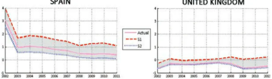
Figure 3 shows the road freight transport trends obtained for the two scenarios simulated (S1 and S2) together with the actual trend, which remains within the grey band delimited by the two scenarios previously mentioned for each country. The growth of intensive-transport sectors in S1 implies a greater road freight transport increase. In the case of Spain, this trend is associated with elasticity values higher than one. On the other hand, for S2, when service GDP share is expanded, road freight transport is progressively detached from GDP, which leads to a clear decoupling trend with elasticity values around 0.1 in this country.
The graph for Spain draws our attention to the fact that road transport volume was above GDP in the three scenarios during the three first years of the study period. The reason explaining the similarity in all the scenarios is that in this period the GDP growth of all the economic sectors was rather small. Along with that fact, in this period road freight transport intensities in Spain grew a lot compared to the base year leading to positive road transport growths when global GDP decreased in all situations (see Fig. 2).
Fig. 3. Real GDP growth and road freight transport trends –∆ veh-kms (%) – under different economic scenarios in Spain (left) and in the United Kingdom (right) from 1999 to 2011.
Looking at the same analysis for the UK, it is seen that road freight growth began to separate from economic growth ever since 2003, accounting for traffic losses of nearly 15% after this year and elasticity values around -0.30. This trend was even more notable after 2007. During the economic crisis traffic reductions greater than 20% were observed compared to the base year. The dematerialization process was almost complete – the actual scenario is close to the S2 scenario. In addition to this fact, the road freight transport intensity in the UK has been declining over the years. These two trends have prompted road transport volume reductions with notable GDP growth ratios.
a higher rate than GDP when considering the hypothesis of the expansion of transport-intensive sectors. In the UK however, this situation for S1 is radically different since the road freight volume remains stable irrespective of the GDP growth.
Figure 4 summarizes the elasticity values obtained for the actual economic evolution, S1 (full materialization) and S2 (full dematerialization). Obviously, the actual elasticities are located within the range defined by the S1 and S2.
Fig. 4. Evolution of the elasticities of veh-km to GDP for the actual evolution of the economy and for scenarios S1 and S2 in the UK and Spain.
Moreover we measure the extent to which the level of dematerialization affects road freight volume for each case study by defining the dematerialization index (ID) through equation (7). This index measures the situation of the
actual scenario compared to Scenarios 1 and 2. Values close to 1 mean that the actual structure of the economy affects road transport volumes as if the economy was almost fully dematerialized.
ܫൌ
ܧௌଵെ ܧ
ܧௌଵെ ܧௌଶ (7)
ES1, ES2 and EA are the averages of the elasticity values during the period of analysis of S1, S2 and the actual
scenarios respectively. The value of the dematerialization index was 0.85 for the UK and 0.68 for Spain.
The comparison of the results obtained for the two countries shows significant differences between them. Firstly, the elasticity values are much lower in the UK than in Spain, and this is related to both a higher dematerialization index in this country and lower RFTI values. This finding allows us to conclude that dematerialization has been one of the key drivers to explain the decoupling trends in this the UK. Nevertheless, this index has also got a value of 0.68 in Spain. This fact confirms that, particularly in the last years of analysis, the loss of material intensity has also contributed to limit road freight transport growth in this country.
Figure 4 also shows that the elasticity range in the UK and Spain for Scenarios 1 and 2 is very different. Looking at the S2 (full dematerialization), this is much lower for the UK than for Spain, even reaching negative values. Figure 4 shows how the UK has attained an almost absolute decoupling level. The different elasticity values in the UK and Spain has been caused by differences in RFTIs between the two countries, as we have already analyzed in section 4 of this paper.
6.Conclusions
This research proves that Input-Output tables combined with transport information at the macro level may be a useful tool for explaining the evolution of road freight transport volume in a certain country. Despite the important progress achieved in the last few years regarding the use of IO tables to model freight transport at the regional and urban scale, IO tables also allow us to obtain interesting conclusions for policy makers by using top-down approaches such as the one we develop in this research, considering each time the validity of the IO data.
restructuring processes lead to the definition of a range where road freight transport could have fluctuated depending on the evolution of the structure of the economy.
In addition, this paper confirms that economic restructuring is not the only driver determining freight transport volume. Other non-economic variables – such as technological, logistic and modal aspects – influencing road freight transport intensities play also an essential role in explaining current and future transport trends.
Finally, for the two country case studies, we can say that the reasons behind the differences in road freight trends during the last few years were two. First, the UK has been a clear example of dematerialization of the economy while Spain was the opposite till the economic recession arrived in 2008. The great dependence of the Spanish economy on construction activities before 2008 entailed high transport volumes within this country. And, secondly, RFTI reductions became a reality in the UK few years earlier than in Spain. This fact helped promote decoupling in the UK while Spain hardly noticed it.
References
Alcántara, V. and Padilla, E. 2003. “Key’ Sectors in Final Energy Consumption: An Input–output Application to the Spanish Case.” Energy
Policy 31 (15): 1673–78. doi:10.1016/S0301-4215(02)00233-1.
Alises, A., Vassallo, J.M. and Guzmán, A.F. 2014. “Road Freight Transport Decoupling: A Comparative Analysis between the United Kingdom and Spain.” Transport Policy 32 (March). Elsevier: 186–93. doi:10.1016/j.tranpol.2014.01.013.
Brunel, J. 2005. “Freight Transport and Economic Growth: An Empirical Explanation of the Coupling in the EU Using Panel Data.”
Cascetta, E., Marzano, V., Papola, A. and Vitillo, R. (2013) A multimodal elastic trade coefficients MRIO model for freight demand in Europe, in: Ben-Akiva, M., H. Meersman and E. Van de Voorde (Eds.) Freight Transport Modelling, Emerald , Bingley.
De la Barra, T. Integrated Land Use and Transport Modeling: Decision Chains and Hierarchies. Cambridge University Press, New York, 1995. Dietzenbacher, E. and Los, B. 1997. “Analyzing Decomposition Analyses.” András Simonovits and Albert E. Steenge (eds.), Prices, Growth and
Cycles. London, Macmillan, 108–31.
Elaurant, S., Ashley, D., Bates, J. 2007. “Future Directions for Freight and Commercial Vehicle Modelling.” In 30th Australasian Transport
Research Forum.
European Union. 2001. WHITE PAPER European Transport Policy for 2010: Time to Decide.
Gerard de J., Gunn, H. and Walker, W. 2004. “National and International Freight Transport Models: Overview for Future Developmemt.”
Transport Reviews 24: 103–24.
Gilbert, R., and Nadeau, K. 2002. “Decoupling Economic Growth and Transport Demand: A Requirement for Sustainability.” In Conference on
Transportation and Economic Development, Transportation Research Board. Portland Oregon.
Hunt, J.D., Abraham, J.E. Design and Application of the PECAS Land Use Modeling System. Presented at the 8th Computers in Urban Planning and Urban Management Conference, Sendai, Japan, 2003.
Hunt, J.D. and Echenique, M.H. Experiences in the Application of the MEPLAN Framework for Land Use and Transportation Interaction Modeling. Proc. 4th National Conference on the Application of Transportation Planning Methods, Daytona Beach, FL, 1993, pp. 723–754. Ivanova, O. (2014) Modelling inter-regional freight demand with input-output, gravity and SCGE methodologies, in: Tavasszy, L. and G. de Jong
(Eds.): Modelling Freight Transport, Elsevier Insights series, Elsevier, London/Waltham.
Kockelman, K.M., Jin, L., Zhao, Y., and Ruiz-Juri, N. Tracking Land Use, Transport, and Industrial Production Using Random-Utility Based Multiregional Input-Output Models: Applications for Texas Trade. Journal of Transport Geography, Vol. 13, No. 3, 2005, pp.
Kveiborg, O., and Fosgerau, M. 2007. “Decomposing the Decoupling of Freight Traffic Growth and Economic Growth 1 Introduction.”
Transport Policy 14: 39–48.
Lehtonen, M. 2008. Energy use in UK road freight : a literature review. Brighton, 1–84.
Lenzen, M., and Foran, B. 2001. “An Input-Output Analysis of Australian Water Usage.” Water Policy 3 (2001): 321–40.
McKinnon, A.C. 2007. “The Decoupling of Road Freight Transport and Economic Growth Trends in the UK : An Exploratory Analysis.”
Transport Reviews 2006
McKinnon, A.C., and Woodburn, A. 1996. “Logistical Restructuring and Road Freight Traffic Growth.” Transportation 23 (2).
doi:10.1007/BF00170033.
OECD. 2002. “Indicators to Measure Decoupling of Environmental Pressure Form Economic Growth”
Schleicher-Tappeser, R., Hey, C. and Steen, P. 1998. “Policy Approaches for Decoupling Freight Transport from.” In 8th World Conference on
Transport Research, 1–20. Antwerp.
Sorrell, S., Lehtonen, M., Stapleton, L., and Pujol, J. 2012. “Decoupling of Road Freight Energy Use from Economic Growth in the United Kingdom.” Energy Policy 41 (February). Elsevier: 84–97. doi:10.1016/j.enpol.2010.07.007.
Tavasszy, L.A. 2006. “Freight Modelling –An Overview of International Experiences.” In TRB Conference on Freight Demand Modelling:
Tools for Public Sector Decision Making, 25–27. Washington DC.
Woxenius, L.J. and Sjöstedt, L. 2003. “Logistics Trends and Their Impact on European Combined Transport - Services , Traffic and Industrial