Modelling and power quality Assessment of an electrolytic cleaning line in the steel making industry

Texto completo

(1)Instituto Tecnológico y de Estudios Superiores de Monterrey Campus Monterrey School of Engineering and Sciences. MODELLING AND POWER QUALITY ASSESSMENT OF AN ELECTROLYTIC CLEANING LINE IN THE STEEL-MAKING INDUSTRY A thesis presented by César Eduardo Suárez Guerrero Submitted to the School of Engineering and Sciences in partial fulfillment of the requirements for the degree of. Master of Science in Energy Engineering. Monterrey, Nuevo León. May 2017.

(2)

(3) Instituto Tecnológico y de Estudios Superiores de Monterrey Campus Monterrey School of Engineering and Sciences The committee members, hereby, certify that have read the thesis presented by César Eduardo Suárez Guerrero and that it is fully adequate in scope and quality as a partial requirement for the degree of Master of Science in Energy Engineering.. ______________________________________ Armando Rafael Llamas Terrés, Ph.D. Tecnológico de Monterrey School of Engineering and Sciences Principal Advisor. ______________________________________ Osvaldo Miguel Micheloud Vernackt, Ph.D. Tecnológico de Monterrey Committee Member. ______________________________________ Raúl Jaime Acosta Cavazos, M.Sc. Ternium México Committee Member. ______________________________________ Rubén Flores O., B.S. Ternium México Committee Member. ______________________________________ Rubén Morales Menéndez, Ph.D. Dean of Graduate Studies School of Engineering and Sciences Monterrey, Nuevo León. May 2017.

(4)

(5) Declaration of Authorship. I, César Eduardo Suárez Guerrero, declare that this thesis titled, “Modelling and Power Quality Assessment of an Electrolytic Cleaning Line in the Steel-Making Industry” and the work presented in it are my own. I confirm that:. •. This work was done wholly or mainly while in candidature for a research degree at this University.. •. Where any part of this thesis has previously been submitted for a degree or any other qualification at this University or any other institution, this has been clearly stated.. •. Where I have consulted the published work of others, this is always clearly attributed.. •. Where I have quoted from the work of others, the source is always given. With the exception of such quotations, this thesis is entirely my own work.. •. I have acknowledged all main sources of help.. •. Where the thesis is based on work done by myself jointly with others, I have made clear exactly what was done by others and what I have contributed myself.. _____________________________________ César Eduardo Suárez Guerrero Monterrey, Nuevo León, May 2017. @2017 by César Eduardo Suárez Guerrero All rights reserved.

(6)

(7) Dedication. To my mother, Lupita To my sisters, Karen and Sofía To my friends and family.

(8)

(9) Acknowledgements I would like to firstly thank my mother Lupita, who has been a paragon of strength, patience, and tenacity all my life. Her support in all my endeavors and decisions has been key in achieving my goals until this point. I also thank my sisters, Karen and Sofía, and my family for their unyielding support of my life endeavors. Thanks to Ternium México for believing in national talent and its potential to make a difference in the current socioeconomic context, and giving me the opportunity to study in such a renowned institution. Thanks to Tecnológico de Monterrey for having the foresight of having programs to attract talented students and professors, and facilitating them the tools needed in order for their research to have meaningful results. I would also like to thank Dr. Osvaldo Micheloud, who trusted me with a scholarship through the Industrial Consortium, and gained my respect by going beyond his due in his support of his students under the belief that nurturing research is something that must be done for the wellbeing and further growth of this country, even being a foreigner himself. Thanks to Dr. Armando Llamas, my mentor while developing this research project. An excellent guide through this challenge, who was always available when the need arose and provided helpful advice and guidance during my studies at this school. He is, undoubtedly, a big part on why this project came to a satisfactory result. Thanks to Raúl Acosta and Rubén Flores from Ternium for taking some of their time to revise and give their opinions about this document. Thanks to all the personnel I had the privilege to interact with at Pesquería Plant, with a special mention to José Luis Bosques for his disposition and commitment to this project while dealing with his daily occupations. A special mention to the people at Ahorro y Calidad de Energía Eléctrica for their helpful advice and support concerning the devices used while developing this thesis. Thanks to my friends at the Consortium for having my back through this journey..

(10)

(11) MODELLING AND POWER QUALITY ASSESSMENT OF AN ELECTROLYTIC CLEANING LINE IN THE STEEL-MAKING INDUSTRY by César Eduardo Suárez Guerrero Abstract This thesis deals with the analysis of the electrical operating conditions in an Electrolytic Cleaning line located inside a relatively new steel-making factory property of Ternium México, and the process to obtain a functional model of the main loads’ circuit using the commercial software MATLAB/Simulink. The motivation for this project was the appearance of several problems in components – whose severity and frequency were not contemplated during the initial design – that were initially believed to stem from Power Quality issues, and a desire to understand the impact that some planned modifications might have in the entire subsystem. In order to validate the data obtained through the simulated model, several pieces of equipment were used to either continuously capture and verify data during normal operation for a period of four weeks or to obtain data at several different occasions during a six-month timeframe. Meanwhile, the aforementioned computer model was being improved by including real-life parameters and characteristics in order to prepare for the eventual simulation. When that was done, the model was fed with data concerning the behavior that devices like an AFE or FOC-based drives would have during normal processing of a roll going through the line. The obtained results were thus contrasted against the actual data obtained by the different measurement devices, producing a discussion centered on the Power Quality attributed of both datasets oriented specifically towards harmonic distortion and its reduction. Finally, several recommendations are given to reduce the effects that were found during the simulation and the various field inspections done during the execution of the project while emphasizing possible avenues of improvement for prospective future work.. VII.

(12) VIII.

(13) List of Figures Figure 1.1. Percent distribution of industrial energy consumption [32] ...................................... 1 Figure 1.2. Steel production schema [31].......................................................................................... 2 Figure 2.1. Graphic representation of both kinds of transient phenomena [11] ......................... 9 Figure 2.2. A momentary fault-induced interruption [11] ........................................................... 10 Figure 2.3. A sag produced by a Single Line to Ground (SLG) fault [11] .................................. 11 Figure 2.4. An instantaneous voltage swell [11]............................................................................ 11 Figure 2.5. Waveform and spectrum content of a full-wave diode rectifier ............................. 12 Figure 2.6. Notching due to electronic device operation [11]...................................................... 13 Figure 2.7. Overcharge/Bonification incentives curve given by CFE formulae [15] ................ 15 Figure 2.8. Skin effect in conductors ............................................................................................... 18 Figure 2.9. PCC distribution example [27] ..................................................................................... 20 Figure 2.10. Space vector .................................................................................................................. 23 Figure 2.11. Sine-triangle modulation ............................................................................................ 26 Figure 2.12. Regular-sampled PWM ............................................................................................... 27 Figure 2.13. SVM sextant with all possible combinations, with an initial reference vector .... 28 Figure 2.14. Three-phase active rectifier with leading LCL filter [14]........................................ 29 Figure 2.15. Basic control scheme in an AFE device [30] ............................................................. 30 Figure 2.16. Basic circuit representation of AFE system, seen from rectifier side .................... 30 Figure 2.17. Main PI controllers involved in AFE operation [25] ............................................... 31 Figure 2.18. Current loop with I/O linearization........................................................................... 33 Figure 2.19. AFE behavior in presence of a voltage notch ........................................................... 34 Figure 2.20. Phase-to-Ground voltage with a 6-pulse rectifier and an AFE.............................. 34 Figure 2.21. DC overvoltage produced by common-mode current [8] ...................................... 35 Figure 2.22. FOC scheme for a three-phase machine ................................................................... 36 Figure 3.1. Main activities of the project ........................................................................................ 37 Figure 3.2. Cold Rolling processes present in Pesquería Plant ................................................... 38 Figure 3.3. Electrolytic Cleaning Line in Steelmaking.................................................................. 39 Figure 3.4. One-line representation of the electrical substation .................................................. 40 Figure 3.5. Shared bus by the mentioned lines .............................................................................. 40 Figure 3.6. Operating values of the transformer ........................................................................... 41 Figure 3.7. AFE Power Circuit [25] ................................................................................................. 42. IX.

(14) Figure 3.8. One-line diagram, AC side ........................................................................................... 43 Figure 3.9. One-line diagram, Tension Reel load ......................................................................... 44 Figure 3.10. Voltage and current waveforms, 100 ms sample .................................................... 45 Figure 3.11. DC bus voltage during a minute sample ................................................................. 45 Figure 3.12. Voltage and current spectrum, 100 ms sample ....................................................... 46 Figure 3.13. Current and voltage probes during measurements................................................ 47 Figure 3.14. Data comparison between PQ sources ..................................................................... 48 Figure 3.15. Harmonic content in both ECL AFE input currents ............................................... 49 Figure 3.16. Comparison between both systems’ Phases A, B, and C, respectively ................ 50 Figure 3.17. Waveform from the main and auxiliary loads, respectively ................................. 51 Figure 3.18. Spectrum from both circuits, with cursor over the 19th harmonic ........................ 51 Figure 3.19. HMI and dedicated device showing PF (a - No load b - Full speed) ................... 52 Figure 3.20. ION measurement devices for the 13.8 kV bus ....................................................... 52 Figure 3.21. Pickling One-Line Diagram (Fragment) ................................................................... 53 Figure 3.22. Waveform and spectrum of Phase A in Pickling .................................................... 53 Figure 3.23. Data stickers placed on the LCL filter....................................................................... 56 Figure 3.24. Electric diagram of current LCL Filter in EC line ................................................... 57 Figure 3.25. Common-mode capacitor condition in EC line ....................................................... 58 Figure 3.26. Common-mode capacitor condition in Pickling line .............................................. 58 Figure 3.27. Data mask for Tension Reel load ............................................................................... 59 Figure 3.28. Inverter portion of the modelled system in Simulink ............................................ 60 Figure 3.29. Internal schematic of modelled motor drive ........................................................... 61 Figure 3.30. DC Bus Conditioner plate data .................................................................................. 62 Figure 3.31. Tension Reel Data during roll processing in ibaAnalyzer ..................................... 63 Figure 3.32. File types accepted as reference ................................................................................. 64 Figure 3.33. Rectifier portion of the modelled system in Simulink............................................ 66 Figure 3.34. Modelled Active Front End control structure ......................................................... 67 Figure 3.35. Interface mask for the LCL filter and the Active Front End .................................. 68 Figure 3.36. DC and Current Controller, and timing compensation in modelled AFE .......... 70 Figure 4.1. Voltage pattern during simulation.............................................................................. 71 Figure 4.2. Current pattern during simulation period ................................................................. 72 Figure 4.3. RMS current during operation .................................................................................... 72. X.

(15) Figure 4.4. Full simulation model ................................................................................................... 73 Figure 4.5. Power Distribution during simulation........................................................................ 74 Figure 4.6. Active and reactive power during roll processing .................................................... 75 Figure 4.7. Simulation Power Factor ............................................................................................... 76 Figure 4.8. Average power factor, per phase ................................................................................. 76 Figure 4.9. LPF operation, 100 ms sample...................................................................................... 77 Figure 4.10. Harmonic spectrum for 100 ms sample during LPF operation ............................. 77 Figure 4.11. HPF operation, 100 ms sample ................................................................................... 78 Figure 4.12. Harmonic spectrum for 100 ms during HPF operation ......................................... 78 Figure 4.13. Simulation results during full speed processing, 100 ms sample ......................... 79 Figure 4.14. Harmonic content during simulation, 100 ms sample during full speed ............ 80 Figure 4.15. DC Voltage and Current ............................................................................................. 80 Figure 4.16. Stator current and Torque, Tension Reel .................................................................. 81 Figure 4.17. Rotor and roll speed, Tension Reel ............................................................................ 81 Figure 4.18. Single phase equivalent of the harmonic circuit ...................................................... 82 Figure 4.19. Voltage amplification according to Equation 4.4 .................................................... 85 Figure 4.20. Frequency response simulation ................................................................................. 85 Figure 4.21. Frequency response results in Simulink ................................................................... 85 Figure 4.22. Wire organization at transformer output ................................................................. 86 Figure 4.23. Damped frequency response ...................................................................................... 87 Figure 4.24. LCL damping switching circuit ................................................................................. 88 Figure 4.25. Currents and harmonic spectrum with no damping resistor ................................ 89 Figure 4.26. Currents and harmonic spectrum with 0.1 Ω damping resistor ........................... 89 Figure 4.27. Currents and harmonic spectrum with a 0.3 Ω damping resistor ........................ 89 Figure 4.28. Three-phase power consumption, 0.1 Ω and 0.3 Ω respectively........................... 90. XI.

(16) XII.

(17) List of Tables Table 2.1. Characteristics of Power Quality phenomena, IEEE 1159-2009 [11]........................... 8 Table 2.2. Characteristic harmonics of rectifier constructions..................................................... 17 Table 2.3. Change in resistance due to skin effect [15]. ................................................................ 19 Table 2.4. Harmonic rotation pattern [15] ...................................................................................... 19 Table 2.5. Voltage distortion limits (IEEE Std 519-2014) [10] ...................................................... 21 Table 2.6. Current distortion levels (120 V – 69 kV) [10] .............................................................. 21 Table 2.7. Current distortion levels (69 kV – 161 kV) [10]............................................................ 22 Table 2.8. Current distortion levels (> 161 kV) [10]....................................................................... 22 Table 3.1. AFE modelling parameters............................................................................................. 54 Table 3.2. Drive parameters ............................................................................................................. 55 Table 3.3. Physical Characteristics of line motors ......................................................................... 56 Table 3.4. LCL Filter electrical data (per-phase)............................................................................ 57 Table 3.5. Transformer impedance data ......................................................................................... 68. XIII.

(18) XIV.

(19) Contents Abstract............................................................................................................................................. VII List of Figures .................................................................................................................................... IX List of Tables .................................................................................................................................. XIII I.. Introduction ................................................................................................................................ 1 1.1.. Description and Objectives for the Work ......................................................................... 3. 1.2.. Structure of the Work.......................................................................................................... 4. II.. Theoretical Framework ............................................................................................................. 7 2.1.. Power Quality ...................................................................................................................... 7. 2.1.1.. Transients...................................................................................................................... 9. 2.1.2.. Voltage Variations ..................................................................................................... 10. 2.1.3.. Imbalance .................................................................................................................... 11. 2.1.4.. Waveform distortion ................................................................................................. 12. 2.2.. Power Factor and Harmonics .......................................................................................... 14. 2.3.. Rectifier and Inverter Configurations............................................................................. 23. 2.3.1.. Space Vectors.............................................................................................................. 23. 2.3.2.. Gate Logic Generation .............................................................................................. 25. 2.3.3.. Active Front End ........................................................................................................ 28. 2.3.4.. Field-Oriented Control Drives ................................................................................. 35. III.. Methodology ......................................................................................................................... 37. 3.1.. Field Data Recollection ..................................................................................................... 38. 3.2.. Data Verification ................................................................................................................ 47. 3.3.. Device Characterization.................................................................................................... 54. 3.4.. Load Modelling.................................................................................................................. 59. 3.5.. Rectifier Modelling ............................................................................................................ 65. XV.

(20) IV.. Results and Discussion ....................................................................................................... 71. 4.1. V. VI.. LCL Filter Resonance ........................................................................................................ 82. Conclusions and Recommendations ................................................................................... 91 Future Work .......................................................................................................................... 93. Annex I ............................................................................................................................................... 95 Annex II ............................................................................................................................................. 97 Annex III ............................................................................................................................................ 99 References........................................................................................................................................ 105 Curriculum Vitae ........................................................................................................................... 109. XVI.

(21) I.. Introduction Energy consumption has been one of the most relevant topics in the last decade. The. increasing focus it has in political and economic circles has put the heat on dedicated research as the general populace shows their preference towards a greener and leaner generation/distribution grid – a tendency that is going to have drastic effects in how the industry manages their own processes to fulfill their own energy and environmental goals, either by law or by self-motivation. Its relevancy comes from the fact that the industrial sector has the biggest share in consumption of end-use energy than any other one, being equivalent to around 54% of the world’s total delivered energy while having a projected growth of 1.2% per year according to data of the U.S. Department of Energy [32]. The biggest part of this surge is expected in the developing world as their industrialization marches on and their integration to the world economy keeps increasing. Of the increasingly complex industrial matrix, several branches are considered as energyintensive: food, pulp and paper, basic chemicals, refining, iron and steel, nonferrous metals, and nonmetallic minerals [32]. As Figure 1.1 shows, together they consolidate half of energy consumption in their category for OECD countries while keeping similar growth patterns for the rest of the world.. Figure 1.1. Percent distribution of industrial energy consumption [32]. 1.

(22) From inspection of the previous graphs, it can be surmised that one of the biggest players when dealing with the use of energy is the iron and steel sector, which captures an average global demand of around 10%. This can be explained when considering the diverse processes involved in this industry to produce each step of the value chain, marking the production of a single roll or slab of steel with a predictably substantial amount of invested energy – either in the form of thermal or electric energy. A glance of how big the steel production grid may become in a company can be seen in Figure 1.2.. Figure 1.2. Steel production schema [31]. But even if the processes are as diversified as shown, there is a constant within this sector and the whole industrial apparatus: electric motors dominate by a large margin the total consumption of electricity. It is estimated that they account between 43% and 46% of all global use of this form of energy, simultaneously leading to an annual amount of emissions around 6,040 Mt of CO2 [34]. When limiting to their uses and applications inside the steelmaking industry, a DOE-commissioned report indicates that they totaled a share of 7% of the total sector energy demand [35]. And as automation marches on, their use will only go up. It is predicted that by 2030 the yearly global consumption will reach 13,360 TWh per year – an increase that is going to be reflected by a ballooning expenditure upwards USD 900 billion just in electricity charges by end-users [34]. And considering that energy represents around 20% of the total steel manufacturing costs, an important increase in energy costs coming from both the introduction. 2.

(23) of specialized equipment and the expected increase in the cost of fuels is boon to eventually make a serious impact in the industry composition and the market [35]. Understanding that, it is not surprising that many of the internal efforts inside companies rely on energy efficiency programs to alleviate this upcoming scenario. It is typical to find them centered around activities such as motor management and maintenance planning, proper sizing of loads (with a preference towards energy-efficient constructions), or power factor correction. Such activities need a deep understanding of the systems involved to recognize how certain modifications and/or configurations can modify its performance, either in a positive or negative way. It is in this context where the focus of the present document clears, which is centered around the analysis of an Electrolytic Cleaning line property of Ternium México, specifically located in Pesquería Plant. As it is a recent operation, it is of interest of the company to understand the reasons behind the situation that has appeared since its initial commissioning. For this work, a Power Quality analysis was done to clarify the conditions in which the line was working at the time, which also doubles as a reference framework to compare against the results of a simulation made in the block-based software Simulink, an element of the MATLAB environment.. 1.1.. Description and Objectives for the Work. Ternium México has codified in its corporate policy the continuous improvement of their production processes, including in those goals an ever-increasing energy efficient workload and the proper management of the involved machinery. Nevertheless, the Electrolytic Cleaning line in its newest industrial complex has shown certain problems that the Electrical Maintenance personnel attribute to a suboptimal design that entails Power Quality events. Although certain modifications have been suggested by the manufacturer of the equipment, it is of their interest to understand and have substantiated evidence of their impact that such changes would have in the general performance of the line. The main objective of this project was to produce a model using the MATLAB/Simulink environment able to reproduce the operational conditions of the main loads corresponding to. 3.

(24) the Electrolytic Cleaning line active in the Pesquería complex, in order to judge how the parameters of the mentioned system interact between them and be able to offer palliatives to undesired developments. To reach that goal, a subset of objectives was defined: •. Define in a clear manner the current situation experienced in the system.. •. Obtain both system parameters and working data during normal operation.. •. Produce an acceptable working model of the system.. •. Compare data from both sources and give recommendations.. 1.2.. Structure of the Work. In this section, a small description of the sections that compose this document is presented to the reader. Chapter 1, the Introduction, mainly deals with the motivations and the scope that encapsulate the current work. How energy has become a bigger issue for the industry and the context that leads to the rise and focus of efficiency programs, specifically in the Iron & Steel sector. The limits of what is going to be touched with the results presented by this document are given to the reader to temper expectations, so the main structure may be rationalized and understood. The Theoretical Framework is explained through Chapter 2, starting with concepts related to Power Quality and the standards related to them, touching upon the characteristics of the events surrounding this concept and how it interacts with the equipment located in the area. Meanwhile, the second part of this section deals with how the electrical power fed to the system passes through different control schemas to be produce the work carrying the production process. More precisely, the fundamentals of both the active rectifier and the inverters feeding the loads are explained to familiarize the reader with the elements composing the simulation.. 4.

(25) The Methodology expanded upon in Chapter 3 encapsulates both the actions taken on site with the physical measurement devices and the development of the model in Simulink in order to successfully characterize the system in question. Also, the reasoning for any differences or conceptions taken during the creation of the model are taken into account through the entire chapter. Chapter 4 is composed of the Results and Discussion part of the document. After obtaining data from real operation and contrasting it with the set obtained through the simulation of a whole process cycle with the model, a discussion of the meaning of what was obtained, the contrasts between reality and the model, and the possibilities concerning the potential improvement of operation are all touched upon. Finally, Conclusions and Future Work are contemplated in Chapter 5 and 6 of the present document, explaining how the objectives were achieved and the recommendations that were reached after the analysis of all recovered data. Failings and prospective work threads are also given for further consideration.. 5.

(26) 6.

(27) II.. Theoretical Framework 2.1.. Power Quality. The concept of Power Quality encapsulates the capacity of an electrical distribution system to feed power to a system without producing undesirable effects while doing so. This becomes important when characterizing the types of loads that are dependent on a power source, with two categories being relevant: •. A load is considered critical when it cannot be disconnected from a voltage source without risking technical and/or economic loses, and potentially endangering human lives [16].. •. A sensitive load can be defined as one with specific needs of a constant supply of voltage and current, with defined characteristics in order for it to work properly [16].. A grid with elements corresponding to either type of load is more sensitive to problems in the voltage or the current circling through the system, making Power Quality events a concern when dealing with the expected performance of a system. Its relevancy only becomes greater when considering the changes in the grids. In the last couple of decades the composition of the interconnected distribution networks has progressively changed, as more nonlinear loads enter (such as computers or drive systems) and affect equipment that was not designed for an erratic grid or needs specific characteristics that may not be found in current operation, resulting from neglected data during the initial analysis or modifications during the timeframe between concept and commissioning. It is desirable to understand how the increasing use of electronics capable of producing electromagnetic disturbances affects sensitive equipment, although segments of both the Electronics and the Power Quality community have used different terms to define the same phenomena [11]. This document uses the widely extended recommended practice published by the Institute of Electrical and Electronics Engineers (IEEE), the Standard 1159, which uses the electromagnetic compatibility concept to describe such phenomena. In said document, a classification for the different Power Quality events was developed, shown in Table 2.1.. 7.

(28) Table 2.1. Characteristics of Power Quality phenomena, IEEE 1159-2009 [11] Categories 1.0. Transients 1.1 Impulsive 1.1.1 Nanosecond 1.1.2 Microsecond 1.1.3 Millisecond 1.2 Oscillatory 1.2.1 Low frequency 1.2.2 Medium frequency 1.2.3 High frequency. Typical spectral content. Typical duration. 5 ns rise 1 μs rise 0.1 ms rise. < 50 ns 50 ns – 1 ms > 1 ms. < 5 kHz 5-500 kHz 0.5-5 MHz. 0.3–50 ms 20 μs 5 μs. 0-4 pu 0-8 pu 0-4 pu. 0.5–30 cycles 0.5–30 cycles. 0.1–0.9 pu 1.1–1.8 pu. 0.5 cycles – 3 s 30 cycles – 3 s 30 cycles – 3 s. < 0.1 pu 0.1–0.9 pu 1.1–1.4 pu. >3 s – 1 min >3 s – 1 min >3 s – 1 min. < 0.1 pu 0.1–0.9 pu 1.1–1.2 pu. > 1 min > 1 min > 1 min > 1 min. 0.0 pu 0.8–0.9 pu 1.1–1.2 pu. steady state steady state. 0.5–2% 1.0–30% 0–0.1% 0–20% 0–2%. broadband. steady state steady state steady state steady state steady state. < 25 Hz. intermittent. 2.0 Short-duration root-mean-square (rms) variations 2.1 Instantaneous 2.1.1 Sag 2.1.2 Swell 2.2 Momentary 2.2.1 Interruption 2.2.2 Sag 2.2.3 Swell 2.3 Temporary 2.3.1 Interruption 2.3.2 Sag 2.3.3 Swell 3.0 Long duration rms variations 3.1 Interruption, sustained 3.2 Undervoltages 3.3 Overvoltages 3.4 Current overload 4.0 Imbalance 4.1 Voltage 4.2 Current 5.0 Waveform distortion 5.1 DC offset 5.2 Harmonics 5.3 Interharmonics 5.4 Notching 5.5 Noise 6.0 Voltage fluctuations. 0–9 kHz 0–9 kHz. 7.0 Power frequency variations. < 10 s. 8. Typical voltage magnitude. 0–1% 0.1–7% 0.2–2 Pst ± 0.10 Hz.

(29) 2.1.1.. Transients. A term used in the analysis of variations in power systems, it implies the notion of a momentary, undesirable event in the power supply. Although there is not a clearly defined limit in what exactly classifies as a transient or not, the most accepted view is that a phenomenon is treated like a transient when its duration is less than a cycle compared to the natural frequency of the studied system [11]. For the phenomena that classifies as such, transients are commonly subdivided according to the waveform of the current or voltage event: •. Impulsive transients are sudden, nonpower frequency changes from the nominal values of voltage, current, or both with unidirectional polarity, characterized by their rise and decay times [11]. Lightning commonly produces this kind of transients, like the one present in Figure 2.1a.. •. Oscillatory transients, on the other hand, are sudden nonpower frequency changes in the steady-state condition of an electrical signal, including positive and negative values [11]. As such, it is described by magnitude, duration, and its spectral content. Capacitor bank maneuvers are often guilty of this type of transients, as seen in Figure 2.1b.. a). b). Figure 2.1. Graphic representation of both kinds of transient phenomena [11]. 9.

(30) 2.1.2.. Voltage Variations. As its name suggests, this category encompasses any variation in the RMS value of voltage in an electrical system. They are almost always caused by faults at some point in the distribution grid, the connection of large loads, or by faulty wiring [11]. Depending on the location of such incidents, the system may experience a dip or a rise compared to the nominal voltage value – sags and swells – or a complete loss of energy – an interruption. An interruption is differentiated from a sag or a swell because it corresponds to a decrease in system voltage equivalent to less than 10% of the nominal [11]. To be considered as momentary or temporary, it cannot endure beyond a minute – otherwise it is treated as permanent (so common protective devices cannot get rid of it) and manual intervention is needed to restore the power supply. Figure 2.2 exemplifies a typical interruption.. Figure 2.2. A momentary fault-induced interruption [11]. Meanwhile, a voltage sag is a decrease in RMS value between 0.1 and 0.9 pu, with durations starting from half a cycle to 1 minute. As the sag category encompasses multiple origin and effect possibilities, terminology can be quite varied; it is preferred to describe them in terms of remaining voltage compared to the nominal value [11]. Usually related to faults, they can also arise from the connection of large loads with high starting currents (See Figure 2.3). If the reduction lasts beyond 1 minute the event is considered an undervoltage, whose typical values hover around 0.8-0.9 pu.. 10.

(31) Figure 2.3. A sag produced by a Single Line to Ground (SLG) fault [11]. In counterpart, a voltage swell is an increase of the RMS value, typically between 1.1-1.2 pu (see Figure 2.4). It is described by the ratio between actual and nominal voltage of the system [11]. If it lingers for more than a minute, it is considered an overvoltage.. Figure 2.4. An instantaneous voltage swell [11]. 2.1.3.. Imbalance. Defined as the ratio of the magnitude of the negative sequence component to the magnitude of the positive sequence component of either voltage or current [11]. It is common to encounter voltage imbalance of around 3%, and it is not strange to find a 30% imbalance between three-phase currents. Its mathematical expression is as follows, shown by Equation 2.1: % 𝐼𝑚𝑏𝑎𝑙𝑎𝑛𝑐𝑒 = |. 𝑉𝑛𝑒𝑔 | ×100 𝑉𝑝𝑜𝑠. (2.1). The standard prefers this definition instead of the one commonly used in measurement devices, which compare the deviation of a voltage against the average phase-to-phase value – exemplified by Equation 2.2. This is because it represents more closely the phenomena of interest, instead of relying in approximations and the error within those operations. (𝑉𝑚 − 𝑉𝑝𝑝 ) % 𝐼𝑚𝑏𝑎𝑙𝑎𝑛𝑐𝑒 = | | ×100 𝑉𝑝𝑝. 11. (2.2).

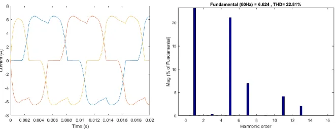
(32) 2.1.4.. Waveform distortion. Like the previous category, it is a steady-state deviation from the ideal, sinusoidal power supply, but in this case the electric variable is mainly characterized by its spectral content [11]. There are 5 primary types of distortion touched upon the IEEE standard. The first case deals with the presence of an injected DC voltage or current in an alternating current system, called DC offset. It can be detrimental due to increases in component saturation, and the heating associated to such development. A second form of distortion is the one produced by the presence of sinusoidal harmonics in either voltage or current, whose frequencies are integer multiples of the system fundamental one (commonly 50 or 60 Hz) [11]. They appear because of the nonlinear nature of loads in the distribution grid, such as any electronically controlled device. The typical distortion of current shown in Figure 2.5 of a diode-based, non-controlled rectifier is one of the simplest examples of the appearance of harmonic content in a network.. Figure 2.5. Waveform and spectrum content of a full-wave diode rectifier. As it is also shown in Figure 2.5, distortion levels produced by harmonics can be characterized by a quantity known as Total Harmonic Distortion (THD). This concept and its implications on system performance will be touched in more detail in the next section.. 12.

(33) Of course, not only integer values of the fundamental frequency produce distortion in the waveform, as other voltages or currents may appear with discrete frequencies or as a spectrum. That kind of distortion is known as interharmonics, and can be found in a variety of networks [11]. Although their effects are not as studied as the ones from harmonics, it is common for their presence to be affecting carrier signaling and be involved in the appearance of flicker events. Continuing with the pattern of power electronics-induced distortion appears the concept of notching, a periodic disturbance that occurs because of the commutation of devices such as diodes, thyristors or IGBTs. This kind of components work in two logic states, and switch their status – in the case they are controlled – at a fast rate. But even at their operation speed they are not completely instantaneous, so there are small periods where there is a short circuit between phases and thus, notching occurs (as seen in Figure 2.6). Their intensity is determined by the source inductance and the insolating inductance between converter, the magnitude of the current and the monitored point.. Figure 2.6. Notching due to electronic device operation [11]. 13.

(34) 2.2.. Power Factor and Harmonics. One relevant quantity for industrial-level machinery is the power factor, which is defined in Equation 2.3 as the ratio between the real and apparent power in a system [15]: 𝑃𝐹 =. 𝑃 𝑆. (2.3). In the case of an ideal sinusoidal power supply – or when dealing with the fundamental frequency – the previous equation can be simplified: 𝑃𝐹 =. 𝑃 𝑉𝐼 cos 𝜃 = 𝑆 𝑉𝐼. 𝑃𝐹 = cos 𝜃. (2.4). Looking to Equations 2.3 and 2.4 it can be surmised that an ideal power factor is unitary, so no reactive power is produced by the source as apparent and real power have the same magnitude. But in the case of inductive and capacitive loads such as motors and transformers the appearance of reactive currents is unavoidable to create the flux that those components need to work – which will inevitably lead to a fall in the power factor for those types of cases. Nevertheless, it is important to maintain a reasonably high (90% or higher) value for the power factor so the system may be optimized while avoiding the penalties carried with the use of energy for unproductive purposes. Such goals are commonly tackled by energy efficiency programs inside the industry, as previously mentioned in the Introduction of the current document. It is common to see actions based on the correction of the power factor in distribution system, comprising but not limited to steps like [15]: •. The detection and replacement of overdimensioned motors.. •. Installing capacitor banks.. •. Installing overexcited synchronous machines.. •. Installing filters, either passive or active.. •. Installing reactive power compensators.. 14.

(35) The reason for such focus in power factor improvement are the benefits obtained when correcting its value. Of those, one of the biggest economic incentives comes in the form of penalizations or bonifications from the power company in the electricity invoice. In Mexico, the biggest player after the aperture of the Electrical Market, Comisión Federal de Electricidad (CFE), applies this measure to their industrial-level loads to promote an efficient and rational use of energy. Using a pair of internal formulas, the company can determine the level of either bonification or overcharge that an individual user will have reflected in their monthly billing, just like Figure 2.7 illustrates.. Figure 2.7. Overcharge/Bonification incentives curve given by CFE formulae [15]. Other of the benefits that comes with the correction of the power factor is the release of capacity used for reactive power, which allows the possibility of using the same equipment with an increase in loading. Also, as less current goes through the conductive elements in the system the I2R losses will inevitably fall. This can be understood by reflecting the changes in the usual loss formula: 𝐼1 =. 𝑃 √3𝑉𝑝𝑝 𝑃𝐹1. ∆𝑃𝑙𝑜𝑠𝑠 = 3(𝐼1 2 − 𝐼2 2 )𝑅 = 3. 𝐼2 = 𝑃. √3𝑉𝑝𝑝 𝑃𝐹2. 2. 3𝑉𝑝𝑝. 15. 𝑃. 2(. 1 𝑃𝐹1. 2. −. 1 𝑃𝐹1 2. )𝑅.

(36) The loss reduction after the improvement of the power factor is:. ∆𝑃𝑙𝑜𝑠𝑠 = 𝑃𝑙𝑜𝑠𝑠1. 𝑃2 1 1 − ( )𝑅 𝑉𝑝𝑝 2 𝑃𝐹1 2 𝑃𝐹1 2 𝑃2 1 ( )𝑅 𝑉𝑝𝑝 2 𝑃𝐹1 2. ∆𝑃𝑙𝑜𝑠𝑠 𝑃𝐹1 2 =1−( ) 𝑃𝑙𝑜𝑠𝑠1 𝑃𝐹2. (2.5). A consideration must be made about the assumptions already done: The displacement angle between real and apparent power is not the only thing that affects the value of the power factor of a system. Harmonic distortion also plays a role in how much energy is used for useful purposes. As it was already mentioned in the previous section, the ever-increasing number of nonlinear loads connected to power systems change the intrinsic sinusoidal shape of the AC current and voltage. This is the direct result of the injection of harmonic currents (and the possibility of voltage distortion) into the system, which may cause malfunctioning in elements sensitive to their presence [10]. This kind of electrical noise can be traced to equipment such as electronic converters, arc furnaces, static VAR systems, cycloconverters, rectifiers, and inverters. Those devices are the most common sources of harmonics found in modern industrial environments – each one of them with their own characteristic spectral behaviors and sensibilities. For the specific case under study, the motor system employs both controlled rectifier and inverter circuits (explained with more detail at the next section). Specifically, as the rectifier is the element that directly interacts with the alternating current power supply, it is of interest to understand its interactions with the AC source. And regardless of its control specifications or the carrier frequency of its gate signal, all rectifiers follow a simple function by which its harmonic generation may be derived [1] [29], shown in Equation 2.6: ℎ = 𝑘𝑝 ± 1. (2.6). Substituting k by any integer number, and replacing p by the number of pulses of the rectifier under study, a specific pattern of harmonics for each kind of energy converter. 16.

(37) appears. Table 2.2 shows the first ten characteristic harmonics of three different AC/DC converter architectures, based on their gate pulses. Table 2.2. Characteristic harmonics of rectifier constructions. Pulses 2 6. 3 5. 5 7. 7 11. 9 13. 12. 11. 13. 23. 25. Harmonics 11 13 17 19 35. 37. 15 23. 17 25. 19 29. 21 31. 47. 49. 59. 61. Of course, there is the possibility to find non-characteristic harmonic values when the system contains undesirable conditions, such as high imbalance in the network, high voltage distortion, or damaged semiconductor components. The presence of even harmonics is not expected in a properly working rectifier when only considering the structure of the device, so an important presence of them (higher than 3% of the fundamental value) may indicate a problem with the converter device [15]. One point to consider when dealing with harmonic content is how much of the demanded current (and voltage) corresponds to the fundamental frequency and is useful, and how much is being wasted in harmonic generation. This may be measured by THD data, mathematically defined in Equation 2.7, and exemplified by currents. √𝐼2 2 + 𝐼3 2 + 𝐼4 2 + ⋯ + 𝐼ℎ 2 𝐷𝑖𝑠𝑡𝑜𝑟𝑡𝑖𝑜𝑛 𝑅𝑀𝑆 %𝑇𝐻𝐷 = = ×100 𝐹𝑢𝑛𝑑𝑎𝑚𝑒𝑛𝑡𝑎𝑙 𝑅𝑀𝑆 𝐼1. (2.7). THD calculation seems to include as many harmonic values as the user desires, but usually they are capped around the 50th order [29]. If higher harmonics are needed for a complete overview the limit may be changed to suit individual cases. Another important concept to consider is the total effect of distortion at the Point of Common Coupling (PCC), known as Total Demand Distortion (TDD). Understood as a percentage of the maximum demand current, it is a ratio of the RMS value of the harmonic content to the RMS of the maximum demand load current, expressed as a percentage of the last value [29]. Its expression is shown in Equation 2.8.. 17.

(38) 2 √∑∞ ℎ=2 𝐼ℎ. %𝑇𝐷𝐷 =. 𝐼𝐿. ×100. (2.8). A large amount of harmonic distortion may not be a problem by itself, but depending of the configuration of a system it may bring havoc to its operation. Even if it is difficult to quantify their effects in a specific manner, they commonly show themselves in several ways: Cables and conductors. When current goes through a conductive element, part of the energy it carries is lost because of the Joule effect (I2R losses), where the current is a function of the current density and the transversal area of the cable. As the frequency of the transmitted signal increases, the effective area of the conductor starts to decrease as the majority of the current tends to be in the outer layer, increasing the heating losses. This phenomenon is called skin effect (see Figure 2.8), and it is only relevant in higher frequencies as those are not really considered by manufacturing [15]. An example in circular conductors is shown in Table 2.3.. Figure 2.8. Skin effect in conductors. Transformers. The majority of transformers are designed to work at fundamental frequency (either 50 Hz or 60 Hz). They have losses by design that are augmented when harmonics enter a system. In the case of the core, these are either due to the mentioned skin effect or by Eddy currents, which are proportional the square of the load current and of the operating frequency.. 18.

(39) Special attention must be put into Δ/Y transformers, as harmonics that correspond to multiples of 3 will only stay in the wye-connection side risking overheating of both windings and the core [15]. Table 2.3. Change in resistance due to skin effect [15].. Conductor size. 60 Hz resistance. 300 Hz resistance. 300 MCM. 1.01. 1.21. 450 MCM. 1.02. 1.35. 600 MCM. 1.03. 1.50. 750 MCM. 1.04. 1.60. Neutral bars. Zero sequence currents, contrary to the case of positive and negative sequence ones, are not cancelled when entering the neutral bars but instead are tripled in a balanced load state – so there is a possibility of overloading them when dealing with nonlinear systems. This may become a problem when the predominant harmonics are in the zero sequence, as a pattern appears when increasing the value of the frequency (see Table 2.4). Table 2.4. Harmonic rotation pattern [15] h. 1. 2. 3. 4. 5. 6. 7. 8. 9. 10. 11. 12. 13. 14. 15. 16. 17. 18. 19. 20. 21. Sequence. +. -. 0. +. -. 0. +. -. 0. +. -. 0. +. -. 0. +. -. 0. +. -. 0. System reactance. The appearance of a harmonic that excites the resonant frequency of the system, either parallel or series, is a problem that may introduce undesired amplification of currents and voltages, as the equivalent admittance steers close to zero. The mentioned heating problems are exacerbated with such phenomenon alongside the needless operation of protective devices or the diminishing lifetime of devices. Knowing the effects of electrical harmonics in equipment and in the overall stability of the distribution system is key to making efforts to diminish their negative impacts. As the management of harmonic distortion is responsibility of both end-users and the controller of the power supply, a middle ground must be reached as the variety of loads keeps increasing. So, considering the impact of their presence in a variety of loads, the IEEE established a recommended practice in their limits as the Standard 519.. 19.

(40) As general goals, the IEEE recommends the levels of distortion shown in Table 2.5 for voltage, while offering the data in Table 2.6, 2.7, and 2.8 for currents at the Point of Common Coupling. The PCC is the point where the customer meets the utility, and it usually corresponds to the point between the utility transformer and the customer’s facility transformer [27]. The standard defines the limits here for several reasons, one being the fact that the Power Company pays and is responsible for all infrastructure behind the PCC, while user bears the costs of their own distribution system. A helpful diagram can be found at Figure 2.9.. Figure 2.9. PCC distribution example [27]. Another reasoning is that going further downstream implies the consideration of local variations that may or may not apply to different systems. As such, the interested parties are encouraged to take such actions as its premise is the reduction of voltage distortion, but if keeping harmonic levels controlled is not enough to favorably modify the situation both players in power delivery should make the necessary changes to have an acceptable power supply [10]. On top of that, another consideration that must be done is that current distortion is based on the ratio between short-circuit current and load current. The short circuit value determines the stiffness of the supply – the higher value of it compared to the nominal current, the higher. 20.

(41) allowed harmonic content [27]. Its value is easily obtained knowing the supply side impedance value and Equation 2.9. 𝐼𝑠𝑐 ≈. 𝑘𝑉𝐴𝑛𝑜𝑚. (2.9). 𝑍𝑠𝑠 , 𝑝𝑢×𝑉𝑠𝑒𝑐𝑜𝑛𝑑𝑎𝑟𝑦 ×√3. As a note to all current related tables, the values shown there only apply to oddnumbered harmonics. For even-numbered ones the standard indicates that a 25% factor must be considered. Table 2.5. Voltage distortion limits (IEEE Std 519-2014) [10]. Bus voltage at PCC. Individual harmonic (%). THD (%). 𝑽 ≤ 𝟏. 𝟎 𝒌𝑽. 5.0. 8.0. 𝟏 𝒌𝑽 < 𝑽 ≤ 𝟔𝟗 𝒌𝑽. 3.0. 5.0. 𝟔𝟗 𝒌𝑽 < 𝑽 ≤ 𝟏𝟔𝟏 𝒌𝑽. 1.5. 2.5. 𝟏𝟔𝟏 𝒌𝑽 < 𝑽. 1.0. 1.5. Table 2.6. Current distortion levels (120 V – 69 kV) [10] 𝑰𝑺𝑪 ⁄𝑰 𝑳. 𝟑 ≤ 𝒉 < 𝟏𝟏. 𝟏𝟏 ≤ 𝒉 < 𝟏𝟕. 𝟏𝟕 ≤ 𝒉 < 𝟐𝟑. 𝟐𝟑 ≤ 𝒉 < 𝟑𝟓. 𝟑𝟓 ≤ 𝒉 < 𝟓𝟎. TDD. < 𝟐𝟎. 4.0. 2.0. 1.5. 0.6. 0.3. 5.0. 𝟐𝟎 < 𝟓𝟎. 7.0. 3.5. 2.5. 1.0. 0.5. 8.0. 𝟓𝟎 < 𝟏𝟎𝟎. 10.0. 4.5. 4.0. 1.5. 0.7. 12.0. 𝟏𝟎𝟎 < 𝟏𝟎𝟎𝟎. 12.0. 5.5. 5.0. 2.0. 1.0. 15.0. > 𝟏𝟎𝟎𝟎. 15.0. 7.0. 6.0. 2.5. 1.4. 20.0. 21.

(42) Table 2.7. Current distortion levels (69 kV – 161 kV) [10] 𝑰𝑺𝑪 ⁄𝑰 𝑳. 𝟑 ≤ 𝒉 < 𝟏𝟏. 𝟏𝟏 ≤ 𝒉 < 𝟏𝟕. 𝟏𝟕 ≤ 𝒉 < 𝟐𝟑. 𝟐𝟑 ≤ 𝒉 < 𝟑𝟓. 𝟑𝟓 ≤ 𝒉 < 𝟓𝟎. TDD. < 𝟐𝟎. 2.0. 1.0. 0.75. 0.3. 0.15. 2.5. 𝟐𝟎 < 𝟓𝟎. 3.5. 1.75. 1.25. 0.5. 0.25. 4.0. 𝟓𝟎 < 𝟏𝟎𝟎. 5.0. 2.25. 2.0. 0.75. 0.35. 6.0. 𝟏𝟎𝟎 < 𝟏𝟎𝟎𝟎. 6.0. 2.75. 2.5. 1.0. 0.5. 7.5. > 𝟏𝟎𝟎𝟎. 7.5. 3.5. 3.0. 1.25. 0.7. 10.0. Table 2.8. Current distortion levels (> 161 kV) [10] 𝑰𝑺𝑪 ⁄𝑰 𝑳. 𝟑 ≤ 𝒉 < 𝟏𝟏. 𝟏𝟏 ≤ 𝒉 < 𝟏𝟕. 𝟏𝟕 ≤ 𝒉 < 𝟐𝟑. 𝟐𝟑 ≤ 𝒉 < 𝟑𝟓. 𝟑𝟓 ≤ 𝒉 < 𝟓𝟎. TDD. < 𝟐𝟎. 1.0. 0.5. 0.38. 0.15. 0.1. 1.5. 𝟐𝟎 < 𝟓𝟎. 2.0. 1.0. 0.75. 0.3. 0.15. 2.5. 𝟓𝟎 < 𝟏𝟎𝟎. 3.0. 1.5. 1.15. 0.45. 0.22. 3.75. 22.

(43) 2.3.. Rectifier and Inverter Configurations. 2.3.1.. Space Vectors. Inverter loads such as induction and synchronous machines, as a consequence of their highly-coupled nature, have led to the creation and adoption of artificial variables rather than using the actual system variables for the sake of simulation and visualization of data [9]. As Figure 2.10 shows, the phase variables can be understood as components of a single vector existing in a three-dimensional orthogonal space which, when projected, give place to the instantaneous values of those same variables.. Figure 2.10. Space vector. Of course, in a balanced three-phase system the sum of those variables is commonly zero as three-phase loads usually lack a neutral return path, making the space limited to a plane referred as the d-q plane. In it, the aforementioned vector is made up of two components, while an axis normal to it – the zero component – exists when the system is imbalanced [9]. Conventionally, the projection of the phase A variable on the plane forms the reference q axis when the axes are not rotating. Equation 2.10 shows the transformation of the three phase variables to the dq0 space.. 23.

(44) 1 𝑓𝑞𝑠 2 [𝑓𝑑𝑠 ] = √ 0 3 𝑓0 1 [√2. 1 2 √3 − 2 1 −. √2. 1 2 𝑓 √3 𝑎 [𝑓𝑏 ] 2 𝑓 𝑐 1 √2 ]. −. (2.10). In the case that the system is balanced, the previous equation is simplified: 3 √ 𝑓𝑞𝑠 2 [𝑓𝑑𝑠 ] = 𝑓0 0 [0. 0. 0. 𝑓𝑎 [𝑓𝑏 ] 1 1 𝑓𝑐 − √2 √2 0 0]. (2.11). So, considering the equations defining a balanced three-phase voltage system: 𝑣𝑎 = 𝑉 sin(𝜔0 𝑡) 2𝜋 𝑣𝑏 = 𝑉 sin (𝜔0 𝑡 − ) 3 2𝜋 𝑣𝑐 = 𝑉 sin (𝜔0 𝑡 + ) 3. (2.12). When analyzing Equation 2.11 with the group of equations shown in Equation 2.12, the transformations can be simplified even further: 3 𝑠 𝑣𝑞𝑠 = √ 𝑉 sin 𝜔0 𝑡 2 𝑠 𝑣𝑑𝑠. 3 = −√ 𝑉 cos 𝜔0 𝑡 2. (2.13). 𝑠 𝑣0𝑠 =0. It can be easily understood that the vector rotates with an angular velocity equal to the angular frequency of the source voltage [9]. The current and flux vector will also describe such trajectory, while having an offset angle to the voltage vector. For the sake of a simplified control of induction motors, more akin to the control of a DC motor, a synchronous voltage reference frame is commonly applied in modern control applications where the defined axes are rotating with the stator voltage. Thus, the. 24.

(45) transformations may be defined as shown in Equation 2.14, divided in two different matrixes for the sake of computational advantage: 𝑓𝑞𝑑0 = 𝑅(𝜃)𝑇𝑞𝑑0 (0)𝑓𝑎𝑏𝑐. (2.14). Where, 2 3 𝑇𝑞𝑑0 (0) = 0. − −. 1 3 1. 1 3 1. −. √3 √3 √2 √2 √2 [3 3 3 ] cos 𝜃 − sin 𝜃 0 𝑅(𝜃) = [ sin 𝜃 cos 𝜃 0] 0 0 1. 2.3.2.. (2.15). (2.16). Gate Logic Generation. Power electronic converters are a family of electrical circuits which convert electrical energy from one level of voltage to another using semiconductor-based electronic switches [9]. Changing the state of said switches in a process called modulation has spawned a number of different control strategies for the better part of 3 decades. One of the most used strategies for controlling the output of power electronic converters is the Pulse Width Modulation technique (PWM), which varies the duty cycle of the switches at a high switching frequency to achieve a lower frequency output. By principle, all modulation schemes aim to create trains of switched pulses with the same fundamental volt-second average as a target reference waveform at any instant [9]. The problem with said trains is the number of harmonics inherent to them. Which makes the main purposes of any modulation scheme the following: 1. Calculate the ON timing which creates the desired output 2. Determine the most effective way of producing the switching process to minimize harmonic distortion.. 25.

(46) For the specific case of PWM, three different alternatives have been proposed for the sake of fixed-frequency modulation [9]: 1. Switching at the intersection of a target reference waveform and a high-frequency carrier, naturally-sampled PWM. 2. Switching at the intersection between a regularly sampled reference waveform and a high-frequency carrier, regular-sampled PWM. 3. Switching so the integrated area of the target reference waveform over the carrier interval is the same as the integrated area of the converted switched input, direct PWM. As for naturally sampled methods, the most common form employed is the one using a triangular carrier in place of a sawtooth one to compare against the reference waveform, as shown in Figure 2.11. This type of carrier modulates both sides of the switched output from the phase leg, improving the harmonic content of the pulse train.. Figure 2.11. Sine-triangle modulation. But a disadvantage of this type of PWM implementation is the difficulty to employ it in a digital modulation system because of the complexity involved in the calculation of the transcendental equation defining the intersection between the reference waveform and the carrier [9]. The regular-sampled PWM method overcomes this limitation by sampling and holding the low-frequency reference during each carrier interval, which is then compared against the triangular carrier to control the switching of each phase leg (see Figure 2.12). The sampled reference must change value at the peak of the reference waveform, in order to avoid the change at the ramping period – a possible cause of multiple switch transitions [9].. 26.

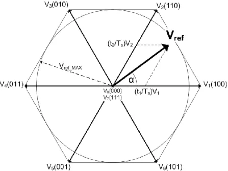
(47) Figure 2.12. Regular-sampled PWM. As for the third method, the determining of the width of the switched pulses is done by switching the inverter to create an active pulse interval for each carrier interval that exactly achieves the same volt-second average of the original target [9]. As the explanation implies, this method requires an integration through the carrier interval, and is usually not practical to implement. An additional alternative for a modulation control technique comes in the form of Space Vector Modulation (SVM), which yields a high voltage gain and less harmonic distortion compared to the earlier mentioned techniques [17]. For the specific case of SVM, the three-phase input currents and output voltages are represented as space vectors, with the algorithm being simultaneously applied to both transformed variables – with the transformation detailed in the previous section, while its magnitude is as shown in Equation 2.17. 2 𝑉0 = [𝑣𝑎𝑏 + 𝑣𝑏𝑐 𝑒𝑗120° + 𝑣𝑐𝑎 𝑒−𝑗120° ] 3. (2.17). The possible switching combinations determine the position of the resulting output voltage space vector (in the case of an inverter) while each combination creates six state space vectors that are used for the synthesis of the output [17], creating the six-sextant hexagon shown in Figure 2.13. The modulation per se involves the selection of the vectors and their on-time computation: During each sampling period, the algorithm selects four active vectors in addition to a zero vector to construct a desired reference voltage – with the specific selection strategy affecting both the harmonic content of the output and switching losses. Then, the amplitude and phase. 27.

(48) angle of the reference are calculated while the desired phase angle of the input current is determined in advance. As for the ON periods of the chosen vectors, they are combined into two sets that lead into two new vectors adjacent to the reference vector in the sextant and having the same direction as the reference [17], while timings are calculated to obtain the component values shown in Figure 2.13.. Figure 2.13. SVM sextant with all possible combinations, with an initial reference vector. 2.3.3.. Active Front End. The dispositive commonly referred as an Active Front End (AFE) in industrial settings can be understood as a power converter structure – which utilizes IGBT modules as switching devices – that usually works as an active rectifier, but may also work as an inverter when feeding power back to the grid [21]. Aside from its regenerative capabilities, when operating as a rectifier this topology basically works as a boost converter [17]. This permits the most desirable characteristics of an AFE device – a boosted DC-link voltage and unity power factor operation. A common structure found in commissioning is displayed in Figure 2.14.. 28.

(49) Figure 2.14. Three-phase active rectifier with leading LCL filter [14]. Initially proposed by Blaabjerg in [4], this kind of topology allows for an achievable sinusoidal input current with THD below 5% [13] [14], but its typical switching frequencies (ranging between 2 and 15 kHz) may cause disturbances that can negatively affect other equipment in the system [5]. To reduce these harmonic currents a high inductance was used in the initial proposal, but at higher power applications it becomes an expensive endeavor while the dynamic response suffers. Because of this, manufacturers tend to include a LCL filter as an alternative [25] [33]. Such filter should be properly designed in order for the circuit to correctly attenuate high-order harmonics while avoiding oscillation effects [14]. So, special attention must be taken with regards to the switching frequency and the resonance point of the circuit – the switching frequency must be high enough to benefit from damping, but also low enough to avoid a bulky and lossy topology [13]. As for the control of this kind of rectifier, space vector transformations are made to the voltage and current signals [24], which are then introduced into a control scheme similar to the one found in Figure 2.15.. 29.

(50) Figure 2.15. Basic control scheme in an AFE device [30]. But before fully delving into the control construct, the basic representation of an AFE should be heeded [21] – the one shown in Figure 2.16. In a rudimentary level, the circuit leading to an AFE may be represented by an AC power source, a series impedance, and a PWM voltage source representing the rectifier. In that case, the dynamic set of equations for the system takes the following form: 𝐸𝑎 𝑖𝑎 𝑉𝑎 𝑑 𝑖𝑎 [𝐸𝑏 ] = 𝐿 [𝑖𝑏 ] + 𝑅 [𝑖𝑏 ] + [𝑉𝑏 ] 𝑑𝑡 𝑖 𝑖𝑐 𝐸𝑐 𝑉𝑐 𝑐. (2.18). Figure 2.16. Basic circuit representation of AFE system, seen from rectifier side. Transforming the previous system of equations into a stationary reference frame: [. 𝑑 𝑖𝑞𝑠 𝐸𝑞𝑠 𝑖𝑞𝑠 𝑉𝑞𝑠 ] = 𝐿 [ ]+𝑅[ ]+[ ] 𝑖 𝑖 𝐸𝑑𝑠 𝑉 𝑑𝑡 𝑑𝑠 𝑑𝑠 𝑑𝑠. 30. (2.19).

(51) Then, taking into consideration the dynamic transformation matrix in Equation 2.16, the system may be transitioned into a reference system rotating at the same angular speed as the electric frequency (With 𝑅(𝜃) becoming 𝐴 for clarity sake): 𝑑 𝐸𝑞𝑠 𝑖𝑞𝑒 𝑖𝑞𝑠 𝑉𝑞𝑠 𝐴 [ ] = 𝐿𝐴 (𝐶 −1 [ ]) + 𝑅𝐴 [ ] + 𝐴 [ ] 𝑖𝑑𝑒 𝑖𝑑𝑠 𝐸𝑑𝑠 𝑉𝑑𝑠 𝑑𝑡 𝑑 𝑑 𝑖𝑞𝑠 𝐸𝑞𝑒 𝑖𝑞𝑒 𝑖𝑞𝑒 𝑉𝑞𝑒 [ ] = 𝐿𝐴 { (𝐴−1 )} [ ] + 𝐿𝐴𝐴−1 {[ ]} + 𝑅 [ ] + [ ] 𝑖 𝑖 𝑖 𝐸𝑑𝑒 𝑉 𝑑𝑡 𝑑𝑡 𝑑𝑠 𝑑𝑒 𝑑𝑒 𝑑𝑒 𝑑 𝑑 𝐸𝑞𝑒 𝑖 𝑖 𝑖𝑞𝑒 𝑉𝑞𝑒 cos 𝜃 − sin 𝜃 cos 𝜃 sin 𝜃 𝑞𝑒 𝑞𝑠 [ ] = 𝐿[ ]{ [ ]} [ ] + 𝐿 {[ ]} + 𝑅 [ ] + [ ] 𝑖𝑑𝑒 𝐸𝑑𝑒 𝑉𝑑𝑒 sin 𝜃 cos 𝜃 𝑑𝑡 − sin 𝜃 cos 𝜃 𝑖𝑑𝑒 𝑑𝑡 𝑖𝑑𝑠 𝑑 𝑖𝑞𝑒 𝐸𝑞𝑒 𝑖𝑞𝑒 𝑉𝑞𝑒 cos 𝜃 − sin 𝜃 −𝜔 sin 𝜃 𝜔 cos 𝜃 𝑖𝑞𝑒 [ ] = 𝐿[ ][ ][ ] + 𝐿 [ ] + 𝑅[ ] + [ ] 𝑖𝑑𝑒 𝐸𝑑𝑒 𝑉𝑑𝑒 sin 𝜃 cos 𝜃 −𝜔 cos 𝜃 −𝜔 sin 𝜃 𝑖𝑑𝑒 𝑑𝑡 𝑖𝑑𝑒 𝑑 𝑖𝑞𝑒 𝐸𝑞𝑒 𝑖𝑞𝑒 𝑉𝑞𝑒 0 1 𝑖𝑞𝑒 [ ] = 𝜔𝐿 [ ][ ] + 𝐿 [ ] + 𝑅[ ] + [ ] 𝑖𝑑𝑒 𝐸𝑑𝑒 𝑉𝑑𝑒 −1 0 𝑖𝑑𝑒 𝑑𝑡 𝑖𝑑𝑒. (2.20). Where Equation 2.20 represents the dynamic model of the system in the d-q plane. Returning to the control discussion, as the AFE intends to work while controlling the power factor, the natural conclusion is that the main control variables will be the current components 𝑖𝑞𝑒 and 𝑖𝑑𝑒 [21] [30]. The q-axis component represents reactive current, and is considered a compensation factor to keep the PF in the desired state; the d-axis component represents the real portion of the current, needed to keep a constant voltage across the DC capacitance and to drive the loads [21]. For the sake of having an optimal control over the system, the current components must be uncoupled from each other, making a feedback loop needed. And for that to occur, both active and reactive current references must be generated; the reactive reference is commonly specified by the user, while the active reference comes from a DC-link controller, as Figure 2.17 illustrates.. Figure 2.17. Main PI controllers involved in AFE operation [25]. 31.

(52) The parameters obtained through the output of the current controller indicate the voltage references that go to the PWM-generation controller, producing the switching logic by any of the previously mentioned methods. Frequency synchronization. An important detail that is common in this kind of control strategies is the need of synchronization with the actual working frequency of the power source – as dq-plane transformations are involved in the generation of the control signals, a slight offset may potentially cause undesirable behavior and flawed feedback, ultimately impacting performance. This kind of control loop is called a phase-locked loop (PLL), and is implemented with the reactive current signal, just as Figure 2.17 shows. Linearization. Another point to consider is the fact that the unbundling of the dynamic equations made by the feedback control loop no longer applies when there are large variations of DC voltage. A large acceleration or deceleration in the loads is a common cause of this kind of behavior [21]. To solve this, new variables referenced to the dynamic description of the system are introduced: ′ 𝑉𝑞𝑒 = 𝑉𝑞𝑒 − 𝐸𝑞𝑒 + 𝜔𝐿𝑖𝑑𝑒 + 𝑖𝑞𝑒 𝑅 ′ 𝑉𝑑𝑒 = 𝑉𝑑𝑒 − 𝐸𝑑𝑒 − 𝜔𝐿𝑖𝑞𝑒 + 𝑖𝑑𝑒 𝑅. (2.21). Substituting them in the dynamic model equations for the rectifier, 𝑑𝑖𝑞𝑒 ′ = −𝑉𝑞𝑒 𝑑𝑡 𝑑𝑖𝑑𝑒 ′ 𝐿 = −𝑉𝑑𝑒 𝑑𝑡 𝐿. (2.22). But even if the current dynamics are now uncoupled, the voltage commands for the PWM controller must consider this change: ∗ ′∗ 𝑉𝑞𝑒 = 𝑉𝑞𝑒 + 𝐸𝑞𝑒 − 𝜔𝐿𝑖𝑑𝑒 − 𝑖𝑞𝑒 𝑅 ∗ ′∗ 𝑉𝑑𝑒 = 𝑉𝑑𝑒 + 𝐸𝑑𝑒 + 𝜔𝐿𝑖𝑞𝑒 − 𝑖𝑑𝑒 𝑅. 32. (2.23).

(53) The current control loop including input linearization is shown in a graphic manner in Figure 2.18.. Figure 2.18. Current loop with I/O linearization. The control that characterizes an Active Front End not only gives them the previously mentioned abilities of working under UPF while boosting the DC voltage, but it also makes them resistant to common Power Quality events. In Figure 2.19 it can be observed the behavior of a common AFE topology in presence of a voltage notch. From the picture, it can be detected that the DC voltage level falls slightly at the same time the current in the faulted phase increases significantly. However, nominal levels of voltage and current recover in less than a cycle [6] [20].. 33.

(54) Figure 2.19. AFE behavior in presence of a voltage notch. Nevertheless, even this kind of device has its own share of problems. As noted in [19], while operating as an active rectifier the phase to ground voltage distortion increases significantly (see Figure 2.20), creating problems with Electromagnetic Compatibility for other loads in the same system in which such characteristics may be critical, such as medical equipment or uninterruptible power supply (UPS) devices [3].. Figure 2.20. Phase-to-Ground voltage with a 6-pulse rectifier and an AFE. Another detail that jumps is the fact that the circulation of line current through the input reactor also generates a large current through neutral to ground, which is filled by high-order frequency content when the AFE is working as an active rectifier. Several topologies have. 34.

(55) been proposed to deal with this fact, usually grounding capacitance in the DC side of the AFE [3] [12]. One more situation that may arise when both uncontrolled rectifiers and AFE share a power supply is the possibility that the common ground current generated by the active system may return through the capacitors in the inverter side of a diode-based rectifier system. This pump-up effect may rise the DC voltage level in the last circuit over design parameters and directly impact the lifetime of the elements connected to it, as seen in Figure 2.21 [8].. Figure 2.21. DC overvoltage produced by common-mode current [8]. 2.3.4.. Field-Oriented Control Drives. Squirrel-cage induction motors (and AC machines in general) historically lacked a control scheme as simple as the one used with a DC machine; doing so would need a decoupling of magnetic flux and produced torque to maintain linearity between inputs and outputs [2]. This problem was overcame with the advent of space vector representations of those machines’ variables, with flux-oriented control strategies allowing their representation in a similar way to the decoupled DC machines. In a DC motor, torque production depends on armature current and machine flux [2], and to produce maximum torque the magnetic field should be maintained at an optimal value (rated flux) while avoiding saturation in the magnetic circuit. That way, the constant flux will. 35.

(56) allow for a linear relationship torque and current. In contrast, when using scalar control in squirrel-cage motors only the stator current is available with no direct way to manipulate the rotor current, making linear control while maintaining maximum torque a difficult proposition to achieve. Field-oriented control makes possible to introduce the same kind of decoupled control by using vector representation, so the relationships between motor variables may be described in a dq-plane rotating with motor flux on the d axis. The basic control scheme used in FOC devices is shown in Figure 2.22.. Figure 2.22. FOC scheme for a three-phase machine. It can be observed that two motor phase currents and the DC-link voltage are measured. The currents are transformed to the stationary reference axes and then to synchronous system, ultimately obtaining rotating components (dq). Those vectors are then compared to reference values obtained through flux and speed controllers, which pass through a controller to become voltage commands. Similar to the gate logic generation in AFEs, the voltage commands are transformed to an appropriate reference system to be used in a Space Vector Modulation schema.. 36.