DOI:10.1051/0004-6361/201628663 c
ESO 2016
Astronomy
&
Astrophysics
Stellar mass function of cluster galaxies at
z
∼
1.5: evidence
for reduced quenching efficiency at high redshift
Julie B. Nantais
1, Remco F. J. van der Burg
2, Chris Lidman
3, Ricardo Demarco
4, Allison Noble
5, Gillian Wilson
6,
Adam Muzzin
7, Ryan Foltz
6, Andrew DeGroot
6, and Michael C. Cooper
81 Departamento de Ciencias Físicas, Universidad Andres Bello, Fernandez Concha 700, 7591538 Las Condes, Santiago,
Regin Metropolitana, Chile e-mail:[email protected]
2 Laboratoire AIM-Paris-Saclay, CEA/DSM-CNRS-Université Paris Diderot, Irfu/Service d’Astrophysique, CEA Saclay,
Orme des Merisiers, 91191 Gif-sur-Yvette, France
3 Australian Astronomical Observatory, PO Box 2915, North Ryde NSW 1670, Australia
4 Departamento de Astronomía, Universidad de Concepción, Casilla 160-C, Concepción, Regin del Biobo, Chile 5 Department of Astronomy & Astrophysics, University of Toronto, Toronto, Ontario M5S 3H4, Canada
6 Department of Physics and Astronomy, University of California-Riverside, 900 University Avenue, Riverside, CA 92521, USA 7 Institute of Astronomy, University of Cambridge, Madingley Road, Cambridge CB3 0HA, UK
8 Department of Physics and Astronomy, University of California, Irvine, 4129 Frederick Reines Hall, Irvine, CA 92697, USA
Received 7 April 2016/Accepted 17 June 2016
ABSTRACT
We present the stellar mass functions (SMFs) of passive and star-forming galaxies with a limiting mass of 1010.1 M
in four
spec-troscopically confirmed SpitzerAdaptation of the Red-sequence Cluster Survey (SpARCS) galaxy clusters at 1.37 < z < 1.63. The clusters have 113 spectroscopically confirmed members combined, with 8–45 confirmed members each. We constructK s-band-selected photometric catalogs for each cluster with an average of 11 photometric bands ranging fromuto 8µm. We compare our cluster galaxies to a field sample derived from a similarKs-band-selected catalog in the UltraVISTA/COSMOS field. The SMFs resemble those of the field, but with signs of environmental quenching. We find that 30±20% of galaxies that would normally be forming stars in the field are quenched in the clusters. The environmental quenching efficiency shows little dependence on projected cluster-centric distance out to∼4 Mpc, providing tentative evidence of pre-processing and/or galactic conformity in this redshift range. We also compile the available data on environmental quenching efficiencies from the literature, and find that the quenching efficiency in clusters and in groups appears to decline with increasing redshift in a manner consistent with previous results and expectations based on halo mass growth.
Key words. galaxies: clusters: general – galaxies: evolution
1. Introduction
The study of galaxy clusters in formation at high redshift (z) is essential to our understanding of the relationship between structure formation and galaxy evolution in the Universe. It is particularly important for understanding how the morphology-density relation (Dressler1980) arose from the earlyz>2 pro-toclusters, which were just beginning to form their red sequences (Kodama et al. 2007; Tanaka et al. 2013). Unlike lower red-shift galaxy clusters, these protoclusters are usually rich in mas-sive, star-forming galaxies (e.g., Overzier et al.2008; Galametz et al. 2010; Hatch et al. 2011a, 2011b; Kuiper et al. 2010; Koyama et al.2013a; Cooke et al.2014; Dannerbauer et al. 2014; Shimakawa et al. 2014; Umehata et al. 2015). However, the galaxies in protoclusters are still affected by their environment. The high-redshift protoclusters are known to show biases with respect to the field in terms of enhanced active galactic nucleus (AGN) activity in their central galaxies (Hatch et al.2014), ex-cesses of high-mass and/or dusty star-forming galaxies with re-spect to the field (Hatch et al. 2011b; Cooke et al.2014), and accelerated chemical evolution (Shimakawa et al.2015). When
compared to lower redshift clusters in terms of their halo masses and galaxy evolution, these protocluster environments show the expected differences in galaxy evolution from their cluster coun-terparts consistent with being the progenitors of the clusters (e.g., Shimakawa et al.2014; Cooke et al.2015).
with both stellar mass and environment (Muzzin et al. 2012; Nantais et al.2013a), and the state of galaxy evolution inz∼1 clusters generally appears to be independent of the selection method (X-ray or infrared) of the galaxy clusters as well (Foltz et al. 2015). In addition to z ∼ 1 being an epoch of en-hanced quenching of cluster galaxies, it is also an epoch of rapid brightest-cluster galaxy growth which parallels that of the cluster halos in general (Lidman et al.2012,2013).
In recent years, the expanding area of research on galaxy clusters and protoclusters in between the above two epochs, at 1.3 <z<2, has shown this intermediate epoch to be an essen-tial phase in galaxy cluster growth. In this redshift range, the role of environment appears to be transitioning between pro-tocluster environmental effects (e.g., growth of massive galax-ies via dusty star formation) and cluster effects (e.g., quench-ing of lower-mass galaxies). Galaxy clusters recognized in and around this epoch often still show substantial star formation in their central regions, unlike clusters at lower redshifts (e.g., Brodwin et al.2013; Fassbender et al.2014; Bayliss et al.2014; Webb et al. 2015a,b). However, environmental quenching is starting to be very important, since many are starting to show substantial red sequences and excesses of quenched galaxies compared to the field, even slightly before this epoch (e.g., Kodama et al.2007; Bauer et al.2011; Quadri et al.2012; Gobat et al.2013; Strazzullo et al.2013; Andreon et al.2014; Newman et al.2014; Balogh et al.2016; Cooke et al.2016). Brightest-cluster galaxy growth is also important at these redshifts, with evidence for both gas-rich mergers (Webb et al. 2015a,b) and gas-poor mergers (Lidman et al. 2012, 2013) contributing to this growth. There are also indications that galaxy evolution correlates with local environment within a forming cluster in this redshift range, as is found at z ∼ 1 (Hatch et al.2016). In order to truly complete our understanding of the evolution of environmental effects on galaxies from protoclusters to ma-ture clusters, we need to study large and, to the extent possi-ble, homogeneously-observed samples of growing high-redshift galaxy clusters at various epochs, rather than a few individual systems.
TheSpitzerAdaptation of the Red-Sequence Cluster Survey (SpARCS; Wilson et al. 2009; Muzzin et al. 2009) has been an excellent resource in high-redshift galaxy cluster re-search, with more than a dozen spectroscopically confirmed, infrared-selected galaxy clusters already reported in the litera-ture (Demarco et al.2010; Muzzin et al.2012,2013a; Lidman et al. 2012, 2013; Webb et al. 2015a,b). Recently-processed data from this survey allow us to expand our knowledge of the critical phases of galaxy cluster evolution with severalz > 1.3 galaxy clusters observed and selected in a manner similar to their lower redshift counterparts. In this paper, we analyze the stellar mass functions and environmental quenching effi cien-cies in a sample of four SpARCS galaxy clusters in the range 1.37 ≤ z ≤ 1.63. The clusters have 113 spectroscopic mem-bers between them, and two of the clusters are described for the first time. We compare these clusters with the state-of-the-art UltraVISTA/COSMOS field sample (Muzzin et al.2013b) in order to discern effects attributable to the cluster environment. In Sect. 2 we describe the photometric and spectroscopic data. In Sect. 3 we describe the methods of photometric and spec-troscopic analysis we used to build our catalogs. In Sect. 4 we describe how we obtained our stellar mass functions. In Sect. 5 we provide the results, and in Sects. 6 and 7 we provide a discus-sion and summary. In this paper, we assume aΛCDM cosmol-ogy withH0 =70 km s−1Mpc−1,ΩM =0.3, andΩΛ =0.7. All
magnitudes used in this paper are in the AB system.
2. Data
Our galaxy clusters were identified using the Stellar Bump Sequence (SBS) technique described in detail in Muzzin et al. (2013a). This infrared selection technique uses the 1.6µm stellar bump, a feature prominent in the rest-frame near-infrared spectral energy distribution of virtually any galaxy containing an underlying stellar population of at least intermediate age (≥100 Myr).
Atz∼ 1.5, the 1.6µm stellar bump conveniently spans the SpitzerInfrared Array Camera (IRAC) 3.6 and 4.5 µm bands, such that galaxies red in [3.6]−[4.5] are likely to be at high redshifts (Papovich2008). Since galaxies at 0.2 < z < 0.4 are also quite red in [3.6]−[4.5], a color cut inz0−[3.6] is made to screen out foreground galaxies atz<0.8 (Muzzin et al.2013a). Using this two-color system, several high-redshift cluster candi-dates were identified within SpARCS and later spectroscopically confirmed.
The spectroscopic data used to confirm the southern clusters and the photometric data used to obtain photometric redshifts, stellar masses, and rest-frame colors are described in the follow-ing subsections. A brief summary of the photometric and spec-troscopic data for each system, plus the number of confirmed members, is shown in Table1.
We show gz[3.6] images of these clusters in Fig. 1, in the same style as their lower redshift counterparts in Wilson et al. (2009) and Muzzin et al. (2009). Objects in white boxes are spectroscopically confirmed cluster members, the bulk of which are small and red (or purple) in these images. Some bright red objects near the centers of clusters lack spectroscopic redshifts despite being targeted in our observing runs, since atz>1.3 it is difficult to obtain the signal-to-noise needed for absorption-line redshifts. Photometric redshifts of these bright red objects show that most have a high probability of being passive cluster mem-bers. The two lower redshift clusters in the top panels of Fig.1, SpARCS-J0335 (z = 1.369, 22 spectroscopic members) and SpARCS-J0225 (z=1.598, 8 spectroscopic members), are being described and analyzed for the first time. The highest-redshift cluster, SpARCS-J0224 (z = 1.633, 45 spectroscopic mem-bers), was featured in Muzzin et al. (2013a). SpARCS-J0224 also appeared in Lidman et al. (2012) along with SpARCS-J0330 (z=1.626, 38 spectroscopic members). Here we extend the anal-ysis of these clusters beyond the few bright cluster members and photometric merger candidates identified in those papers.
2.1. Spectroscopy
Spectroscopy of high-redshift cluster member candidates was performed with the Focal Reduction and Imaging Spectrograph 2 (FORS2; Appenzeller & Rupprecht1992) on the European Southern Observatory (ESO) Very Large Telescope (VLT) Unit Telescope 1 (UT1) in Mask Exchange Unit (MXU) mode for all four clusters. The spectroscopy was performed in four separate service-mode programs. Total on-target integra-tion time ranged from 40 min to four hours. Data reducintegra-tion was performed with the customized software described in Nantais et al. (2013b) for FORS2 MXU data.
For SpARCS-J0330, SpARCS-J0224, and SpARCS-J0225, near-infrared multi-object spectroscopy was obtained with the MOSFIRE spectrograph on the Keck Telescopes in Hawaii in several observing runs (PI G. Wilson). Comparison of MOSFIRE vs. FORS2 redshifts for overlapping objects in SpARCS-J0224 and SpARCS-J0330 suggests an uncertainty of
Table 1.SpARCS high-redshift data summary.
Cluster RA (J2000) Dec (J2000) z Spectroscopy Photometry Spec. members
h:m:s d:m:s
SpARCS-J0224 02:24:26.33 –03:23:30.8 1.633 FORS2, MOSFIRE, OzDES ugrizY JK s3.6µm 4.5µm5.8µm 8.0µm 45 SpARCS-J0330 03:30:55.87 –28:42:59.5 1.626 FORS2, MOSFIRE, OzDES ugrizY JK s3.6µm 4.5µm5.8µm 8.0µm 38 SpARCS-J0225 02:25:45.55 –03:55:17.1 1.598 FORS2, MOSFIRE, OzDES ugrizY K s3.6µm 4.5µm5.8µm 8.0µm 8 SpARCS-J0335 03:35:03.58 –29:28:55.6 1.369 FORS2, OzDES grizY K s3.6µm4.5µm 5.8µm 8.0µm 22
N
E N
E
N
E
N
E
Fig. 1.Tri-colorgz[3.6] images of the central regions of the four southernz>1.35 SpARCS clusters, with 40×
40
fields of view. Spectroscopic cluster members are marked with white squares, and the orientation of the image is shown in the lower left corner of each cluster image.
similar to that found in Nantais et al. (2013b) for FORS2 spec-troscopy of az=1.2 galaxy cluster, and lower than the velocity dispersion expected for galaxy clusters at these redshifts.
Additional spectroscopy exists for all fields in the Australian Dark Energy Survey (OzDES; Yuan et al.2015). OzDES targets typically lie at lower redshift than these clusters. However, one redshift is of a cluster member, a bright AGN in the outskirts of SpARCS-J0335. The remainder of the OzDES redshifts, at
z<1, are very useful for checking our photometric redshifts and improving their quality.
2.2. Imaging
The imaging data were collected with ground- and space-based facilities and cover a wavelength range that, for most clusters, extends from the observer-frame u band (0.35 µm) to 24 µm (with Spitzer MIPS). In our analysis, we use the data out to IRAC 8 µm. Three of the four clusters were observed in the optical with the f/2 camera of the Inamori-Magellan Areal Camera & Spectrograph (IMACS; Dressler et al. 2011) on the Magellan Baade telescope during two observing runs, one in September 2011 and the other in December 2012. The fourth cluster, SpARCS J0225, lands within the deep D1 field ob-served by the Canada-France-Hawaii Telescope (CFHT) Legacy Survey1(CFHTLS) and therefore has deep coverage in the opti-cal with MegaCam on CFHT. All four clusters were observed in the near-infrared with the High Acuity Wide-field K band Imager (HAWK-I; Pirard et al.2004; Casali et al.2006) on the ESO VLT in service mode over three ESO periods.
The clusters were also imaged with IRAC on the Spitzer Space Telescope, first as part of theSpitzerWide-area Infrared Extragalactic Survey (SWIRE; Lonsdale et al.2003) in all four IRAC bands, and then later with deeper observations in the IRAC 3.6 and 4.5µm bands as part of theSpitzerExtragalactic Representative Volume Survey (SERVS).
2.2.1. IMACS and CFHTLS data processing
The IMACS data were processed in a standard manner using our own scripts that called IRAF2tasks.
SCAMP (Bertin2006) and SWarp (Bertin et al.2002)3were
used to map the sky-subtractedz-band images onto the astromet-ric reference frame defined by bright stars in the USNO-B1 cat-alog. The internal residuals reported by SCAMP were typically 0.0300 or less. We used thesez-band images as the astrometric reference for all other images taken with IMACS and HAWK-I. The uncertainties in the zero points vary from 1% inito 5% inu. For SpARCS-J0225, we used the CFHTLSi-band image as the astrometric reference due to incomplete areal coverage in the zband.
2.2.2. HAWK-I data processing
The processing of the raw HAWK-I data was also done in a stan-dard manner and largely follows the steps outlined in Lidman et al. (2008,2012). SCAMP and SWarp were used to map the sky-subtracted images onto the astrometric reference frame de-fined by the bright stars in thez-band images that were taken with IMACS. After accounting for irregularities such as gain varia-tions, bad pixels, and satellite trails, the images were then com-bined with the IMCOMBINE task within IRAF. Each image was weighted with the inverse square of the full width at half maxi-mum (FWHM) of the point spread function (PSF) to maximize the image quality of the final combined image.
With the exception of the data taken in theY band, zero-points were set using stars from the Two-Micron All-Sky Survey (2MASS) point source catalog (Skrutskie et al.2006). ForY, the zeropoint was set using standard stars that were observed during 1 We used version 7 of the reduced images, which are available from
http://terapix.iap.fr
2 IRAF is distributed by the National Optical Astronomy
Observatories which are operated by the Association of Universities for Research in Astronomy, Inc., under the cooperative agreement with the National Science Foundation.
Fig. 2.Ks-band detection completeness fraction as a function of total
Ks magnitude for the four southern cluster fields. The red circles rep-resent SpARCS-J0224; the orange triangles reprep-resent SpARCS-J0330; the yellow stars represent SpARCS-J0225; and the blue circles repre-sent SpARCS-J0335. The black dash-dot line reprerepre-sents the 90% cutoff for determining the completeness limit.
the same night as the clusters. The uncertainties in the zeropoints are generally less than 2%, and more typically 1%, for bothJand Ks.
Before performing multi-color photometry, all processed op-tical, HAWK-I, and IRAC data were transformed to a common pixel scale using SWARP to facilitate photometry. The final scale of all images was 0.18500pixel−1.
2.2.3. Data quality, including image depth
Over all, the image quality of the ground-based imaging data varies from 0.300 FWHM forKs-band data taken with HAWK-I to 1.100FWHM foru-band IMACS data.
Ks-band detection completeness limits were calculated using a methodology similar to that used for UltraVISTA in Muzzin et al. (2013b). The ten brightest non-saturated PSF stars in each field were used to make a model PSF in the Ks-band images (transformed to the 0.18500 pixel−1 scale, but without adjust-ments of image quality) using the IRAF DAOPHOT package. This PSF was then dimmed to create artificial point sources. Two thousand copies of these point sources were superimposed upon theKs-band detection images in random locations. An ar-tificial point source was considered detected if (a) a detection was made within one pixel (0.18500) of its true location and (b) this detection did not coincide with a preexisting source in the Ks-band detection images. Our method corresponds to the re-alistic scenario of Muzzin et al. (2013b), accounting for losses due to overlap with bright stars and poor-quality regions of the image. With it, we estimate a maximum completeness of 99% at Ks<21 mag AB.
the 90% completeness limits for consistency with van der Burg et al. (2013).
3. Photometric and spectroscopic analysis
3.1. Photometric catalog creation
The photometric catalogs were created following procedures similar to those of Muzzin et al. (2013b) for UltraVISTA. Objects were detected in the sameKs-band images as were used for the completeness using Source Extractor (Bertin & Arnouts 1996) version 2.19.5. Astrometric and pixel-scale matching was performed on all images using SWarp prior to photometry.
To determine colors, PSF matching was performed with con-volution kernels created with the IRAF taskwiener4 on all im-ages. The PSFs of optical and ground-based near-infrared bands were matched to the poorest image quality among these bands.
Photometry for color determination was measured in aper-ture diameters of 2.200 in the u through Ks bands and 3.700 in the IRAC bands using Source Extractor in dual-image mode. Correction factors for Ks-IRAC colors were calculated in a manner similar to Muzzin et al. (2013b) and van der Burg et al. (2013).
All photometry intended for science is corrected for Galactic extinction (reddening) using Schlegel et al. (1998) dust maps and Schlafly & Finkbeiner (2011) extinction corrections. Extinction values were very low in the infrared, less than 0.01 mag in the Ks band and IRAC, and low to moderate in the optical: 0.02– 0.05 mag in theiband and 0.03–0.09 mag in thegband.
We estimated the photometric uncertainties via the fluctua-tions of background levels in up to 5000 empty apertures, similar to the methodology of Labbé et al. (2003), with non-empty aper-tures rejected at the extremes of the flux distribution. Additional uncertainties of 5% of the flux for IRAC and 1% of the flux for optical through Ks were added to account for zeropoint uncer-tainties.
The zeropoints for the multi-wavelength aperture photome-try were tested and, if need be, corrected using the stellar locus (High et al.2009) as compared to Covey et al. (2007) and stars in the GCLASS catalogs. The adjustments (1–10%) roughly matched the uncertainties (up to a few percent) in most bands, but were sometimes larger inJandKs. These larger offsets were still comparable to those of Muzzin et al. (2013b), in which Ks-band corrections were about 8%. Integrated photometry in Ks-band was determined using Source Extractor’s MAG_AUTO parameter, with an aperture correction (typically around 4%) de-termined using artificial stars of known flux.
3.2. Photometric redshift and rest-frame color estimation
Photometric redshifts and rest-frame UV J colors were calcu-lated using the EAZY code (Brammer et al. 2008). Stellar masses were estimated using the FAST code (Kriek et al.2009). Parameters for EAZY and FAST were based on those used in van der Burg et al. (2013), and the EAZY parameters in particu-lar were chosen to minimize the scatter in photometric redshifts. FAST stellar mass outputs were based on Bruzual & Charlot (2003) [BC03] models.
4 The taskwienerapplies a non-iterative Fourier deconvolution filter
chosen from one of four varieties: inverse, Wiener, geometric mean, or parametric. The default fitting parameters with a Wiener filter, recom-mended by the authors of the task for restoring stellar images, were used to calculate the convolution kernels from our stars.
0.0 0.2 0.4 0.6 0.8 1.0 1.2 1.4 1.6 1.8
z_phot vs. z_spec, 1 Mpc Radius
Fig. 3.Photometric vs. spectroscopic redshift for the inner 1 Mpc sam-ple of galaxies in the four cluster fields. The normalized median abso-lute deviation (NMAD) and outlier rates are included in the figure.
Figure 3shows the photometric vs. spectroscopic redshifts for galaxies up to 1 Mpc from the cluster center in all four clus-ter fields. Redshifts significantly beyond those of the highest-redshift clusters are virtually absent, given that the spectral fea-tures needed to confirm redshifts fall outside our FORS2 and MOSFIRE windows at z ∼ 1.7. The scatter (normalized me-dian absolute deviation or NMAD) of (zphot−zspec)/(1+zspec)
(excluding outliers) is σ = 0.04, comparable to van der Burg et al. (2013). Our outlier rate within this region, defined as per-centage of objects with (zphot−zspec)/(1+zspec)≥0.15 as in van
der Burg et al. (2013), is 5.4%, slightly higher than in van der Burg et al. (2013). Outlier rates without cluster-centric distance constraints increase by about a factor of 3 due to inclusion of more faint objects, but this has little effect on typical photomet-ric redshift quality. Redshifts above those of the highest-redshift clusters are nearly absent since the spectral features needed to confirm redshift fall out of the optical and near-IR windows of our spectroscopic data.
The stellar masses derived from FAST allowed us to de-termine stellar-mass completeness limits corresponding to our Ks-band completeness limits. Following the example of van der Burg et al. (2013), we determine these stellar-mass limits as be-ing the highest stellar mass of any UltraVISTA galaxy at ourK s-band completeness limit near the cluster redshift. In Table2we show the stellar mass limits determined for each cluster, featured in Col. 4.
3.3. Photometric members and comparison samples
We define photometric membership for our clusters as (zphot−
zcl)/(1+zcl) ≤ 0.05, following van der Burg et al. (2013),
af-ter adjusting the photometric redshifts by (zphot−zcl)/(1+zcl)=
+0.02 to account for a slight systematic offset. Our photometric membership cut-offclosely matches the scatter of our photomet-ric redshifts (σ ∼ 0.04). We exclude objects near bright stars from our photometric member sample.
Table 2.Stellar mass completeness limits.
Cluster Redshift Ks limit Log mass limit Mass function limit
mag log(M/M) log(M/M)
Fig. 4. Rest-frame UV J colors for photometric and spectroscopic cluster members (red dots), shown with the color distribution for UltraVISTA field galaxies of the same stellar mass and photometric redshift as the clusters (gray scale in units of arbitrarily normalized UltraVISTA galaxy counts). Solar-metallicity Bruzual & Charlot (2003) complex stellar population evolutionary tracks are displayed with vari-able age steps (15 000 yr to 0.25 Gyr) out to 4.5 Gyr (which corresponds to the age of Universe atz=1.37). The red model represents a single burst and the blue, green, and black models represent exponentially de-clining star formation with increasing levels of internal reddening.
The rest-frame UV J color–color diagram for photometric and spectroscopic cluster members and UltraVISTA field galax-ies, which indicates the passive vs. star-forming distinction (Wuyts et al. 2007; Williams et al. 2009; Patel et al.2012), is shown in Fig. 4. The cluster galaxies (confirmed and uncon-firmed) are shown as red dots, while the arbitrarily normal-ized, stellar-mass-matched UltraVISTA field galaxy counts are shown in gray scale. The rest-frame UV J colors of the cluster galaxies appear to be generally well-matched to the UltraVISTA field galaxy distribution, suggesting similar accuracy in the color determination. The passive fractions are also similar, though slightly higher in the cluster sample: 45% of the spectroscopic and photometric cluster members are passive vs. 39% of the field galaxies.
4. Determination of stellar mass functions
To determine stellar mass functions, we followed a methodol-ogy based on van der Burg et al. (2013). We defined seven stel-lar mass bins starting at 1010.1 M separated by 0.2 dex, and estimated the total number counts (spectroscopic members plus photometric members minus field counts) in each bin within 1 Mpc of the cluster center. In each cluster, the cluster center is defined as the position of the brightest (inKs) galaxy located
in the region with the highest surface density of photometric and spectroscopic members. Spectroscopic member counts are given a Poisson uncertainty, while photometric member counts are given an uncertainty based on 100 Monte Carlo simulations of photometry varied within its error margins. In the two lowest stellar mass bins, the total counts are corrected for the fraction of clusters complete in these bins.
Because of the bias in our spectroscopic selection, in which false positives for photometric membership outweigh false neg-atives due to easy confirmation of bright red star-forming fore-ground galaxies, the spectroscopy-based field contamination correction factors of van der Burg et al. (2013) are inappropri-ate for our data. We therefore corrected the photometric clus-ter members for field contamination by estimating field galaxy counts within (zphot−zcl)/(1+zcl) ≤ 0.05 of the cluster
cen-ter and subtracting these counts, yielding a correction indepen-dent of the quality of spectroscopy. We use the full UltraVISTA data to correct for the estimated field galaxy counts in each clus-ter, scaling the total counts to match the survey volume for each cluster.
We correct for field counts separately for passive and star-forming galaxies by subtracting the passive galaxy field counts from the passive stellar mass function and the star-forming field counts from the star-forming stellar mass function. Passive and star-forming galaxies are each divided into three V − J color bins and added together in order to make the total passive and star-forming stellar mass functions, and all color bins for both passive and star-forming galaxies are added together to make the total stellar mass functions. With our methodology, we obtain the same total stellar mass functions regardless of whether or not we treat the passive and star-forming galaxies separately. Similarly, the division of passive and star-forming galaxies into multiple color bins gives the same overall passive and star-forming stellar mass functions as would treating all passive and all star-forming galaxies as a single entity.
Uncertainties in field counts are estimated by resampling the UltraVISTA field in the areas and redshift ranges of all four clus-ters (equivalent to 4πMpc2in projected area) in 1000 random lo-cations, and taking the standard deviation of the total field counts (for all four clusters) in these 1000 samplings as the sampling un-certainty in the field corrections. Again, this is done separately for passive and star-forming galaxies as well as for the full sam-ple combined. The uncertainties from field sampling are similar in value to the field counts themselves, and are added in quadra-ture to the cluster galaxy count errors. The field sampling uncer-tainty contributes moderately to the error margins in the stellar mass functions and the passive and star-forming fractions, and strongly to the uncertainty in the environmental quenching effi -ciency (discussed in Sect. 5.2).
clusters. In fact, in all four clusters, theKs-band BCG is either not the most massive galaxy or is tied for the most massive with a fainter galaxy. In contrast, only 3 of the 10 similarly analyzed z<1.35 GCLASS clusters have a BCG that is not also the most massive cluster galaxy according to our team’s unpublished data. Therefore, the evolutionary processes that would create extraor-dinary BCGs that deviate from the Schechter function have not yet occurred in our high-redshift clusters.
The seven stellar mass bins with total photometric and spec-troscopic cluster member counts and uncertainties are fitted with a Schechter function using a maximum-likelihood method. Since we do not account for asymmetrical error bars in the num-ber counts, this fit is basically equivalent to least-squares fit-ting. However, in determining uncertainties in the stellar mass function itself, we do choose to take into account the asymme-tries in the error bars. We use emcee (Foreman-Mackey et al. 2013) to perform Monte Carlo simulations of various fluctua-tions around the maximum-likelihood parameters φ∗ (normal-ization), log (M∗) (characteristic mass), andα(faint-end slope). We take the 1σuncertainties to be the difference between the best-fit values and the lower and upper limits (marginalizing over other parameters) of each parameter for all simulated re-sults with (ln(Lmax)−ln(L)) < 0.5, following van der Burg
et al. (2013), where Lis the likelihood function for the given set of fit parameters.
The UltraVISTA stellar mass functions are estimated as in van der Burg et al. (2013) as the number of galaxies per stellar mass bin per co-moving cubic megaparsec, with Poisson uncer-tainties. The survey volume was estimated to be 1.09×10⁷Mpc3
in the redshift range 1.251 <z < 1.765, which corresponds to |(zphot−zcl)/(1+zcl)| ≤0.05 of the lowest- and highest-redshift
clusters. In the lowest stellar mass bin, only the SpARCS-J0335 redshift range was considered, and the counts in this bin were corrected for the fraction of survey volume coverage.
5. Results
Below we discuss the stellar mass functions and their uncertain-ties for the clusters and the field, and estimate the environmental quenching efficiency of the clusters.
5.1. Stellar mass functions
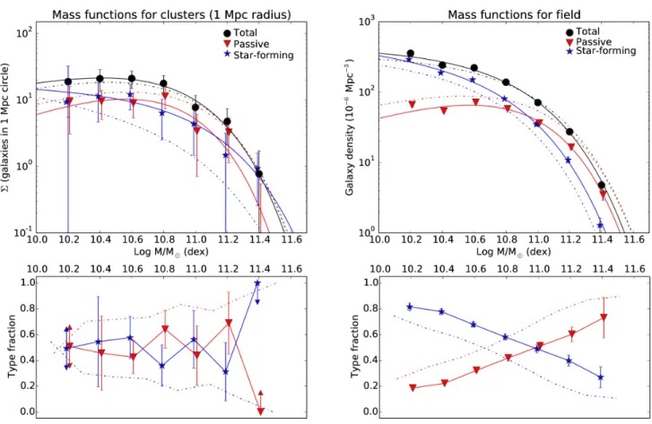
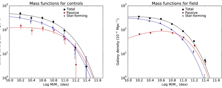
The stellar mass functions for the total, passive, and star-forming galaxy populations are shown in Fig.5, with the cluster stellar mass functions on the left and the field stellar mass functions on the right. The van der Burg et al. (2013) stellar mass function fits and type fractions, normalized to match our data, are shown as dash-dot lines. Type fractions (passive in red, star-forming in blue) based on rest-frameUV Jcolors are shown below the stel-lar mass functions in Fig.5, with uncertainties in type fractions for the clusters derived from the same Monte Carlo simulations as were used to estimate the uncertainties in galaxy counts.
The shape of the total stellar mass function is virtually iden-tical between the cluster and field, within 1.1σ. In the field, the passive component is dominant at high stellar masses, while the star-forming component clearly dominates at low masses. In the clusters, however, passive galaxies make up roughly 50% of the total even at low masses, as opposed to only 20% at low masses in the field (29% in total), indicating the importance of environmental quenching. Throughout most of the range, the passive and star-forming fractions remain within 1σof one an-other in the clusters. In the highest-mass bin there is only a single
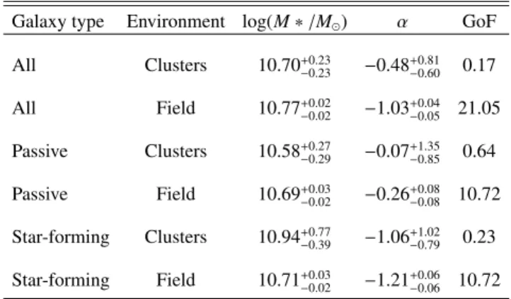
Table 3.Stellar mass function parameters.
Galaxy type Environment log(M∗/M) α GoF
star-forming galaxy, an unconfirmed photometric member, and therefore its presence does not allow us to draw any definitive conclusions about the high-mass end of the stellar mass func-tion. In the Schechter function fit, its main effect is to increase the uncertainty inM∗.
When comparing to the van der Burg et al. (2013) curves (dash-dot lines), both the cluster and the field show quenching betweenz∼1 andz∼1.5. The quenching is much more drastic in the clusters, where passive galaxies become heavily dominant at nearly all stellar masses at the lower redshifts. The total mass functions, however, change very little betweenz∼1.5 andz∼1, apart from a modest increase in high-mass galaxies seen in the field.
Table3summarizes the results of the parameter fits for log M∗ and α and gives a reduced χ2 goodness-of-fit (GoF)
esti-mate5. All uncertainties in Table3 are based on the lower and upper limits from Monte Carlo simulations of parameter sets in which (ln(Lmax)−ln(L)) <= 0.5. The M∗ andαvalues agree
within 1σbetween the clusters and the field. Both the clusters and the field have shallowαfor the passive galaxies and similar, steeperαfor star-forming galaxies. The values in the table, like the figures, generally support the notion of similar stellar mass functions for both the cluster and the field, for star-forming and passive galaxies alike.
5.2. Cluster quenching efficiency
We estimate the total corrected passive and star-forming counts from the binned data and use these in the environmental quench-ing efficiency formula6 employed by various other researchers
(van den Bosch et al. 2008; Peng et al.2012; Wheeler et al. (2014); Kawinwanichakij et al.2016; Balogh et al.2016). The environmental quenching efficiency, also called conversion frac-tion or environmentally-quenched fracfrac-tion, is tradifrac-tionally de-fined as follows:
feq=(fpassive,dense−fpassive,field)/(1−fpassive,field). (1)
5 The large GoF values in the field are driven by the small fractional
uncertainties in galaxy counts (Poisson or scaled Poisson) as compared to their deviations from the Schechter function, such that the Schechter function appears to under-fit the data. The small GoF values in the clus-ters are driven by large fractional uncertainties in galaxy counts due to small number counts and large uncertainties from photometry, such that the Schechter function appears to over-fit the data.
6 We do not employ the van der Burg et al. (2013) method of fitting
Fig. 5.Stellar mass functions for cluster (left) and field (right) galaxies, showing both the data and the best Schechter function fits (top) and the type fractions in each mass bin (bottom) with red representing passive galaxies and blue representing star-forming galaxies. The dash-dot lines represent stellar mass functions and type fractions from van der Burg et al. (2013) normalized to match our data. Arrows for error bars represent unconstrained type fractions in a stellar mass bin. Passive and star-forming stellar mass data are offset horizontally by±0.01 dex for clarity.
In this equation, feq is the environmentally-quenched fraction,
fpassive,denseis the passive fraction in the dense environment
(clus-ter, protoclus(clus-ter, group, or filament), and fpassive,fieldis the
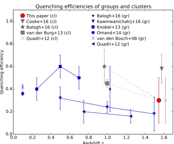
pas-sive fraction in the field. In our data, we obtain an environmental quenching efficiency of 30±20%, similar to Quadri et al. (2012) for theirz∼1.6 cluster.
Our result for the environmental quenching efficiency is higher than (but consistent with) the typical 20% environmental quenching efficiencies around passive central galaxies atz∼1.5 in Kawinwanichakij et al. (2016), but lower than (yet still con-sistent with) the environmental quenching efficiency of 45% ob-tained atz ∼1 in van der Burg et al. (2013) and the quenching efficiencies of 40% and 60% found by Balogh et al. (2016) for groups and clusters atz ∼ 1 respectively. Our results therefore suggest environmental quenching effects intermediate between rich clusters atz ∼ 1 and groups at z ∼ 1.5, although the un-certainties (driven largely by the field subtraction) do not allow statistical confirmation of this possibility.
Cooke et al. (2016) do not calculate an environmental quenching efficiency directly for their z ∼ 1.6 high-redshift cluster, but among all galaxies above 1010 M, 70±13% were
deemed to be quenched in their high-redshift cluster, vs. only 28% in the UDS control field. This would suggest an environ-mental quenching efficiency of 58%, higher than the van der Burg et al. (2013) value and comparable to the rich cluster value in Balogh et al. (2016). However, this is based on only 29±6 excess galaxies, with very few spectroscopic members. Given the quoted uncertainty in the original quenched fraction, the
uncertainty of the Cooke et al. (2016) environmental quenching efficiency would make it consistent with the results of van der Burg et al. (2013).
6. Discussion
6.1. Robustness of results
In order to test the robustness of our results, we considered three important aspects of our sampling that might affect our stellar mass functions: (1) the areal extent of the cluster sample; (2) the redshift range of confirmed members; and (3) the correction for estimated field galaxy counts.
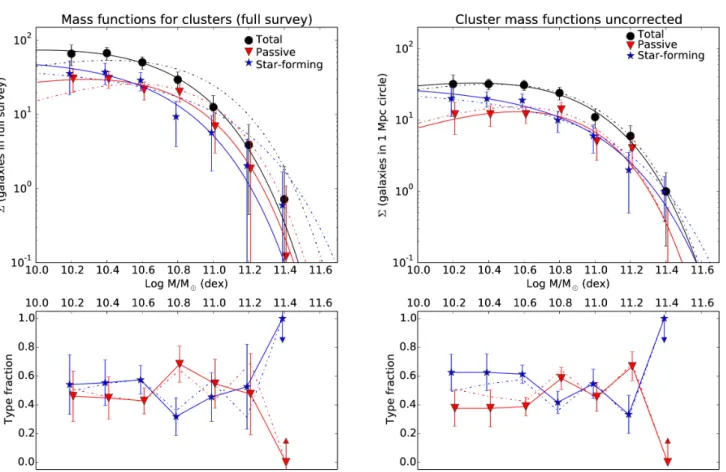
Although we consider only the inner megaparsec for consis-tency with van der Burg et al. (2013), we may be excluding a large number of infalling galaxies which may be undergoing en-vironmental pre-processing. According to Muldrew et al. (2015), a network of galaxies spanning 50 co-moving megaparsecs in di-ameter atz∼2 may be destined to become part of az=0 clus-ter. Atz =1.6, the upper limit would correspond to a radius of about 9 (proper) Mpc for a massive cluster, which is larger than the area we probe. We therefore check whether the inclusion of more distant infalling cluster members (both photometric and spectroscopic) would change our results.
Fig. 6.Similar to Fig. 5, but with theleft panelsshowing the cluster stellar mass functions removing cluster-centric distance constraints and the
right panelsshowing the cluster stellar mass functions in the inner 1 Mpc without field correction. The dash-dot lines represent our original results normalized to match the reanalysis.
higher within 1 Mpc than in the full survey, indicating that galax-ies in the cluster outskirts are predominantly faint. The passive and star-forming fractions, however, are essentially unchanged. The full survey yields an environmental quenching efficiency of 27%±10%, almost identical to our previous result (with smaller percent error due to much higher low-mass galaxy counts and a lower percent uncertainty from field subtraction).
To double-check the quenching efficiency results at large projected distances, we estimated the environmental quenching efficiency for all galaxies farther than 1 Mpc from the clus-ter cenclus-ters. We still found a value of 25±16% for the clus-ter outskirts when correcting for field galaxies (though only 10±4% without such corrections). We rule out the possibility that the SpARCS-J0225 foreground sheet alone is mimicking pre-processing in the cluster outskirts, since excluding this clus-ter actually increases the environmental quenching efficiency of the cluster outskirts.
The above result has several possible explanations: (a) pre-processing of the low-mass galaxies in the cluster out-skirts; (b) general galactic conformity (Weinmann et al. 2006; Kauffmann et al.2013; Kauffmann 2015; Hearin et al.2015); (c) rapid quenching after having crossed the cluster even once (Wetzel et al.2013); or (d) difficulty distinguishing photometri-cally between passive and star-forming galaxies at the faint mag-nitudes typical of the cluster outskirts. We note the representative error bar inU−Vcolor in Fig.4for galaxies within 1 Mpc, which includes nearly all the bright galaxies. Regardless of the reason for this, however, including galaxies at larger cluster-centric dis-tances does not affect our result, and thus we have no reason
to discount our results on the basis of excluding distant, star-forming cluster members.
We also tested our results with a smaller sample of galax-ies within the central 0.5 Mpc, in case the original 1 Mpc limit included too many non-members and recent infalls to show the full extent of environmental effects. We obtained nearly the same environmental quenching efficiency (31%±26%) as within a 1 Mpc radius.
Our next test addressed our spectroscopic member redshift cutoff. The original redshift cutoffs correspond to 3σof a rich cluster’s velocity dispersion, which could be considered overly generous for a low-mass, non-virialized cluster (discounting complex superstructure along the line-of-sight). We re-analyze the data with redshift cutoffs of±0.0075 from the cluster center atz∼1.6 and±0.008 atz=1.37, half the previous values. These cutoffs still contain 50–87% of the original spectroscopic mem-bers of each cluster, but span a maximum line-of-sight diameter of 18–19 Mpc. The narrower redshift cutoffhas no significant effect on mass function shapes or environmental quenching effi -ciency, raising the latter insignificantly to 31±22%.
0.0
0.2
0.4
0.6
0.8
1.0
1.2
1.4
1.6
Redshift z
0.0
0.2
0.4
0.6
0.8
1.0
Quenching efficiency
This paper (cl)
Cooke+16 (cl)
Balogh+16 (cl)
van der Burg+13 (cl)
Quadri+12 (cl)
Balogh+16 (gr)
Kawinwanichakij+16 (gr)
Knobel+13 (gr)
Omand+14 (gr)
van den Bosch+08 (gr)
Quadri+12 (gr)
Quenching efficiencies of groups and clusters
Fig. 7.Environmental quenching efficiencies as a function of redshift for our high-redshift cluster sample (large red circle) and various other group and cluster samples in the literature. Dash-dot lines connect related studies and solid lines connect results from the same study. Slight offsets between studies at the same redshift with overlapping error bars have been added for clarity.
The right panels of Fig. 6 show the 1 Mpc cluster sam-ple with no corrections for field contamination, with our orig-inal result shown as dash-dot lines. The result is similar to the original but with less similarity in type fraction between pas-sive and star-forming cluster galaxies at low masses. The en-vironmental quenching efficiency in the uncorrected sample is 20%±6%, matching the Kawinwanichakij et al. (2016) value for groups around passive galaxies atz ∼1.5. If we repeat this no-field-correction analysis in the central 0.5 Mpc, the environ-mental quenching efficiency for the uncorrected sample rises to 26%±8%, approaching the value of∼30% consistently found after correcting for field galaxy counts. The quenching efficiency values without field subtraction have much higher confidence (3σas opposed to 1.5σ) due to not including the large uncer-tainties from field counts. Therefore, we have high confidence in our main conclusions that (a) the cluster stellar mass functions are generally similar to the field, but with evidence of increased quenching relative to the field at low masses and (b) the environ-mental quenching efficiency of our clusters is lower than what is found in clusters atz∼1 but comparable to or higher than that of groups atz∼1.5.
We leave for Appendix A a final check on the robustness of our results: the comparison of field galaxies in UltraVISTA with the most pristine field galaxies of our own survey.
6.2. Environmental quenching efficiencies and evolution of dense environments
The intuitive picture of galaxy evolution that we would expect is that galaxies in clusters, protoclusters, and groups are quenched
more efficiently over time, so that environmental quenching effi -ciencies at low redshifts would exceed those at high redshifts in a given category of local density or halo mass. Gerke et al. (2007) found some evidence of this when comparing the blue fractions of group galaxies at 0.75 < z < 1.3. The blue fractions in the groups were lower than in the field atz ≤ 1, but byz ∼ 1.3 they were identical to field values. Butcher & Oemler (1984) and more recent studies such as Haines et al. (2013) have found sim-ilar effects in rich galaxy clusters at low-intermediate redshifts.
In Fig.7we compare the environmental quenching efficiency of our high-redshift cluster sample with various environmental quenching efficiencies estimated from other studies of groups and clusters at various redshifts, with their references given in the legend. The group samples are represented by blue symbols and the cluster samples are represented by gray symbols. Our sample is represented by the large red circle.
The quenching efficiencies appear to vary mostly by halo mass category (groups vs. clusters), but within each halo mass category, there are signs of a decrease in environmental quench-ing efficiency with increasing redshift, with groups and clusters atz ∼1.5 having quenching efficiencies about 10% lower than their similarly-selected counterparts at z . 1. Such a trend is consistent with the earlier findings of Gerke et al. (2007) and Haines et al. (2013).
independent of the stellar mass of the galaxy (Wetzel et al.2013; De Lucia et al. 2014; Hirschmann et al.2014; Phillips et al.2014; Fillingham et al.2015; Wheeler et al. 2014). Furthermore, in-terstellar medium research suggests that higher redshift galax-ies use up their gas very quickly (e.g., PHIBSS: Tacconi et al. 2013; Genzel et al. 2012,2015; Saintonge et al.2013), an effect that may enhance quenching efficiency at high redshift if the gas supply is suddenly shut off. Therefore, some other factor, such as the average amount of time spent in the cluster environment per galaxy, may lead to reduced environmental quenching effi -ciencies at high redshift.
When interpreting Fig. 7 we note that the environmental quenching efficiency does not take into account the estimated epoch of infall of the galaxies in a cluster, and the evolution of the quenched fraction in the field – its lower value at higher red-shift – since that epoch. Therefore, environmental quenching ef-ficiencies at lower redshifts may be underestimates of the true impact of the environment, if the galaxies in groups and clusters at low redshifts were accreted at higher redshifts and thus more likely to be star-forming before entering the cluster. However, it is also possible that the galaxies that were accreted into clusters were pre-processed in groups beforehand, and thus were more quenched than typical field galaxies at their infall time, balanc-ing this effect (McGee et al.2009).
7. Summary
We analyzed the stellar mass functions of passive and star-forming galaxies down to 1010.1Min a set of four
spectroscopi-cally confirmed, infrared-selected galaxy clusters from SpARCS at 1.37 <z <1.63, with a total of 113 spectroscopic members and an extensive catalog of photometric redshifts, stellar masses, and rest-frame colors from an average of 11 optical to infrared bands. Our major results were as follows:
The shape of the total stellar mass function of the galaxy clusters resembles that of the field. The shapes of the passive and star-forming stellar mass functions also resemble those of the field, although there is less difference between their rela-tive dominance at both high and low masses in the galaxy clus-ters. That is, in the galaxy clusters the passive and star-forming fractions are close to 50% at all stellar masses, whereas in the field passive galaxies are dominant at the highest stellar masses and star-forming galaxies are highly dominant at low stellar masses. This difference between clusters and field is more sig-nificant at low stellar masses. The environmental quenching effi -ciency, or conversion fraction, of our clusters was estimated to be 30±20%, intermediate between high-redshift groups atz∼1.5 and galaxy clusters atz∼1.
The above results were found to be robust with respect to cluster-centric distance, spectroscopic redshift cuts for cluster membership, and corrections for field contamination. The ro-bustness of type fractions and conversion fraction with respect to cluster-centric distance may be a signature of galactic con-formity or group and filament pre-processing. Not correcting for field contamination led to a modest decrease in the environmen-tal quenching efficiency, but it differed significantly from zero and had a value comparable to high-redshift groups, which in-creased our confidence in our results.
A compilation of environmental quenching efficiency data from the literature indicates a decrease in environmental quench-ing efficiency in groups and clusters with increasing redshift, with a drop of about 10% between z . 1 and z ∼ 1.5. This finding is consistent with previous research at intermediate red-shifts finding less difference between groups and clusters and the
field at higher redshifts than at lower ones. Since related research suggests that galaxies should quench faster at higher redshifts (Balogh et al.2016) and quenching is not strongly related to halo mass within a given redshift range, this result may be due to the galaxies in higher redshift groups and clusters, having spent, on average, significantly less time in the cluster environment than in lower redshift clusters.
Acknowledgements. Based in part on observations obtained with MegaPrime/MegaCam, a joint project of CFHT and CEA/DAPNIA, at the Canada-France-Hawaii Telescope (CFHT), which is operated by the National Research Council (NRC) of Canada, the Institut National des Sciences de l’Univers of the Centre National de la Recherche Scientifique (CNRS) of France, and the University of Hawaii. This work is based in part on data products produced at TERAPIX and the Canadian Astronomy Data Centre as part of the Canada-France-Hawaii Telescope Legacy Survey, a collaborative project of NRC and CNRS. Based in part on observations taken at the ESO Paranal Observatory (ESO programs 085.A-0166, 085.A-0613, 086.A-0398, 087.A-0145, 087.A-0483, 088.A-0639, 089.A-0125, and 091.A-0478). Based in part on observations taken at the Las Campinas Observatory in Chile. Based in part on observations taken at the Keck Telescopes in Hawaii. Based in part on observations made with the Spitzer Space Telescope, which is operated by the Jet Propulsion Laboratory, California Institute of Technology under a contract with NASA. During the course of this project, JN received funding from FONDECYT postdoctoral research grant no. 3120233 and Universidad Andres Bello internal research project DI-651-15/R. This research has made use of the VizieR catalog access tool, CDS, Strasbourg, France. R.D. gratefully acknowledges the support provided by the BASAL Center for Astrophysics and Associated Technologies (CATA), and by FONDECYT grant No. 1130528. R.F.J.v.dB. acknowledges support from the European Research Council under FP7 grant number 340519. M.C.C. acknowledges support from NSF grant AST-1518257. G.W. acknowledges financial support for this work from NSF grant AST-1517863 and from NASA through programs GO-13306, GO-13677, GO-13747 & GO-13845/14327 from the Space Telescope Science Institute, which is operated by AURA, Inc., under NASA contract NAS 5-26555.
References
Andreon, S., Newman, A., Trinchieri, G., et al. 2014,A&A, 565, A120
Appenzeller, I., & Rupprecht, G. 1992,The Messenger, 67, 18
Balogh, M., McGee, S., Mok, A., et al. 2016,MNRAS, 456, 4364
Bauer, A., Grtzbauch, R., Jorgensen, I., Varela, J., & Burgmann, M. 2011,
MNRAS, 411, 2009
Bayliss, M., Ashby, M., Ruel, J., et al. 2014,ApJ, 794, 12
Bertin, E., & Arnouts, S. 1996,A&AS, 117, 393
Bertin, E., Mellier, Y., Radovich, M., et al. 2002, ASP Conf. Ser. 281, eds. D. A. Bohlender, D. Durand, & T. H. Handley, 228
Bertin, E. 2006, in ASP Conf. Ser. 351, eds. C. Gabriel, C. Arviset, D. Ponz, & E. Solano, 112
Brammer, G., van Dokkum, P. G., & Coppi, P. 2008,ApJ, 686, 1503
Brodwin, M., Stanford, S. A., Gonzalez, A. H., et al., 2013,ApJ, 779, 138
Bruzual, G., & Charlot, S. 2003,MNRAS, 344, 1000
Butcher, H., & Oemler, A. 1984,ApJ, 284, 426
Casali, M., Pirard, J., Kissler-Patig, M., et al. 2006,Proc. SPIE, 6269, 29
Cooke, E., Hatch, N., Muldrew, S., Rigby, E., & Kurk, J. 2014,MNRAS, 440, 3262.
Cooke, E., Hatch, N., Rettura, A., et al. 2015,MNRAS, 452, 2318
Cooke, E., Hatch, N., Stern, D., et al. 2016,ApJ 816, 83
Covey, K., Ivezi´c, Z., Schlegel, D., et al. 2007,AJ, 134, 2398
Dannerbauer, H., Kurk, J., De Breuck, C., et al. 2014,A&A, 570, A55
De Lucia, G., Weinmann, S., Poggianti, B., Aragón-Salamanca, A., & Zaritsky, D. 2012,MNRAS, 423, 1277
Demarco, R., Wilson, G., Muzzin, A., et al. 2010,ApJ, 711, 1185
Dressler, A. 1980,ApJ, 236, 251
Dressler, A., Bigelow, B., Hare, T., et al. 2011,PASP, 123, 288
Fassbender, R., Nastasi, A., Santos, J., et al. 2014,A&A, 568, A5
Fillingham, S., Cooper, M., Wheeler, C., et al. 2015,MNRAS, 454, 2039
Foltz, R., Rettura, A., Wilson, G., et al. 2015,ApJ, 812, 138
Foreman-Mackey, D., Hogg, D., Lang, D., & Goodman, J. 2013,PASP, 125, 306
Galametz, A., Vernet, J., De Breuck, C., et al. 2010,A&A, 522, A58
Genzel, R., Tacconi, L., Combes, F., et al. 2012,ApJ, 746, 69
Genzel, R., Tacconi, L., Lutz, D., et al. 2015,ApJ, 800, 20
Gerke, B., Newman, J., Faber, S., et al. 2007,MNRAS, 376, 1425
Gobat, R., Strazzullo, V., Daddi, E., et al. 2013,ApJ, 776, 9
Hatch, N., De Breuck, C., Galametz, A., et al. 2011a,MNRAS, 410, 1537
Hatch, N., Kurk, J., Pentericci, L. et al. 2011b,MNRAS, 415, 2993
Hatch, N., Wylezalek, D., Kurk, J., et al. 2014,MNRAS, 445, 280
Hatch, N., Muldrew, S., Cooke, E., et al. 2016,MNRAS, 459, 387
Hearin, A., Watson, D., & van den Bosch, F. 2015,MNRAS, 452, 1958
High, F. W., Stubbs, C. W., Rest, A., Stalder, B., & Challis, P. 2009,AJ, 138, 110
Hirschmann, M., De Lucia, G., Wilman, D., et al. 2014,MNRAS, 444, 2938
Kauffmann, G. 2015,MNRAS, 454, 1840
Kauffmann, G., Li, C., Zhang, W., & Weinmann, S. 2013,MNRAS, 430, 1447
Kawinwanichakij, L., Quadri, R., Papovich, C., et al. 2016,ApJ, 817, 9
Knobel C., Lilly, S., Kovac, K., et al. 2013,ApJ, 769, 24
Kodama, T., Tanaka, I., Kajisawa, M., et al. 2007,MNRAS, 377, 1717
Koyama, Y., Kodama, T., Tadaki, K., et al. 2013a,MNRAS, 428, 1551
Koyama, Y., Smail, I., Kurk, J., et al. 2013b,MNRAS, 434, 423
Kriek, M., van Dokkum, P., Labbé, I., et al. 2009,ApJ, 700, 221
Kuiper, E., Hatch, N., Röttgering, H., et al. 2010,MNRAS, 405, 969
Labbé, I., Franx, M., Rudnick, G., et al. 2003,AJ, 125, 1107
Lidman, C., Rosati, P., Tanaka, M., et al. 2008,A&A, 489, 981
Lidman, C., Suherli, J., Muzzin, A., et al. 2012,MNRAS, 427, 550
Lidman, C., Iacobuta, G., Bauer, A., et al. 2013,MNRAS, 433, 825
Lonsdale, C. J., Smith, H. E., Rowan-Robinson, M., et al. 2003,PASP, 115, 897
McGee, S., Balogh, M., Bower, R., Font, A., & McCarthy, I. 2009,MNRAS, 400, 937
Muldrew, S., Hatch, N., & Cooke, E. 2015,MNRAS, 452, 2528
Muzzin, A., Wilson, G., Yee, et al. 2009,ApJ, 698, 1934
Muzzin, A., Wilson, G., Yee, H. K. C., et al. 2012,ApJ, 746, A188
Muzzin, A., Wilson, G., Demarco, R., et al. 2013a,ApJ, 767, A39
Muzzin, A., Marchesini, D., Stefanon, M., et al. 2013b,ApJS, 206, A8
Muzzin, A., van der Burg, R., McGee, S., et al. 2014,ApJ, 796, A65
Nantais, J., Flores, H., Demarco, R., et al. 2013a,A&A, 555, A5
Nantais, J., Rettura, A., Demarco, R., et al. 2013b,A&A, 556, A112
Newman, A., Ellis, R., Andreon, S., et al. 2014,ApJ, 788, 51
Noble, A., Webb, T., Muzzin, A. et al. 2013,ApJ, 768, 118
Noble, A., Webb, T., Yee, H., et al. 2016,ApJ, 816, 48
Omand C. M. B., Balogh M. L., & Poggianti B. M. 2014,MNRAS, 440, 843
Overzier, R., Bouwens, R., Cross, N., et al. 2008,ApJ, 673, 143
Papovich, C. 2008,ApJ, 676, 206
Patel, S. G., Holden, B. P., Kelson, D. D., et al. 2012,ApJ, 748, L27
Peng, Y., Lilli, S., Renzini, A., & Carollo, M. 2008,MNRAS, 387, 79
Pirard J.-F., Kissler-Patig, M., Moorwood, A, et al. 2004,Proc. SPIE, 5492, 1763
Phillips, J., Wheeler, C., Cooper, M., et al. 2014,MNRAS, 442, 1396
Quadri, R., Williams, R., Franx, M., & Hildebrandt, H.2012, ApJ, 744, 88
Saintonge, A., Lutz, D., Genzel, R., et al. 2013,ApJ, 778, 2
Schechter, P. 1976,ApJ, 203, 297
Schlafly, E. and Finkbeiner, D. 2011,ApJ, 737, A103
Schlegel, D., Finkbeiner, D., & Davis, M. 1998,ApJ, 500, 525
Shimakawa, R., Kodama, T., Tadaki, K., et al. 2014,MNRAS, 441, 1L
Shimakawa, R., Kodama, T., Tadaki, K., et al. 2015,MNRAS, 448, 666
Skrutskie M. F., Cutri, R. M., Stiening, R., et al., 2006,AJ, 131, 1163
Strazzullo, V., Gobat, R., Daddi, E., et al., 2013,ApJ, 772, 118
Tacconi, L., Neri, R., Genzel, R., et al. 2013,ApJ, 768, 74
Tanaka, M., Toft, S., Marchesini, D., et al. 2013,ApJ, 772, 113
Umehata, H., Tamura, Y., Kohno, K., et al. 2015,ApJ, 815, 8
van den Bosch, F., Aquino, D., Yang, X., et al. 2008,MNRAS, 387, 79
van der Burg, R. F. J., Muzzin, A., Hoekstra, H., et al. 2013,A&A, 557, A15
Webb, T., Noble, A., DeGroot, A., et al. 2015a,ApJ, 809, 173
Webb, T., Muzzin, A., Noble, A. et al. 2015b,ApJ, 814, 96
Weinmann, S., van den Bosch, F., Yang, X., & Mo, H. 2006,MNRAS, 366, 2
Wetzel, A. R., Tinker, J. L., Conroy, C., & van den Bosch, F. C. 2013,MNRAS, 432, 336
Wheeler, C., Phillips, J., Cooper, M., et al. 2014,MNRAS, 442, 1396
Williams, R. J., Quadri, R. F., Franx, M., van Dokkum, P., & Labbé, I. 2009,
ApJ, 691, 1879
Wilson, G., Muzzin, A., Yee, H., et al. 2009, ApJ, 698, 1943
Wuyts, S., Labbé, I., Franx, M., et al. 2007,ApJ, 655, 51
Appendix A: SpARCS vs. UltraVISTA field galaxies
As a final check on the robustness of our results, we com-pare the stellar mass functions of SpARCS and UltraVISTA field galaxies to look for any important systematic differences. For the SpARCS data, we define field galaxies as objects with 1.251 < z < 1.487 (SpARCS-J0335 photometric redshifts) in the SpARCS-J0330 and SpARCS-J0224 fields. This avoids cluster-outskirts members within J0330 and SpARCS-J0224. We exclude SpARCS-J0225 from the field galaxy anal-ysis because any foreground sample may include members of thez =1.43 sheet which might differ from pristine field mem-bers. We also exclude SpARCS-J0335 due to the shallow optical photometry for this cluster making it impossible to distinguish between passive and star-forming z ∼ 1.6 background galax-ies. In the UltraVISTA field, we also consider only objects with 1.251 < z < 1.487 to compare to our SpARCS field galaxies, to ensure that the co-moving line-of-sight distance and state of galaxy evolution in the field are equivalent in both samples.
To construct the stellar mass function for SpARCS field galaxies, we take the average counts in each stellar mass bin in our 100 Monte Carlo simulations with photometric redshift and stellar mass results varied according to uncertainties in the photometry. Averaging the simulated results, as opposed to using
Fig. A.1.Stellar mass functions for SpARCS foreground control galaxies (left) and UltraVISTA (right) field galaxies at 1.251<z<1.487. Passive and star-forming stellar mass data are offset by±0.01 dex in stellar mass for clarity.
the original counts only, helps reduce variations due to small-number statistics, except in the two highest mass bins in which the SpARCS foreground field samples are most deficient. These highest mass bins would be expected to be occupied largely by brightest group and cluster galaxies, whereas the SpARCS field subsample was selected to be free of known groups and clusters. Stellar mass functions were fit the same way as for the clusters and for the field in the main analysis.
![Fig. 1. Tri-color gz[3.6] images of the central regions of the four southern z > 1.35 SpARCS clusters, with 4 0 × 4 0 fields of view](https://thumb-us.123doks.com/thumbv2/123dok_es/3779009.646874/3.892.100.794.293.970/color-images-central-regions-southern-sparcs-clusters-fields.webp)