DOI:
10.1051
/
0004-6361
/
201527511
Mapping the outer bulge with RRab stars from the VVV Survey
F. Gran
1,2, D. Minniti
3,2,4, R. K. Saito
5, M. Zoccali
1,2, O. A. Gonzalez
6,7, C. Navarrete
1,2, M. Catelan
1,2,
R. Contreras Ramos
2,1, F. Elorrieta
8,2, S. Eyheramendy
8,2, and A. Jordán
1,21 Instituto de Astrofísica, Pontificia Universidad Católica de Chile, Av. Vicuña Mackenna 4860, 782-0436 Macul, Santiago, Chile
e-mail:[email protected]
2 Millennium Institute of Astrophysics, Santiago, Chile
3 Departamento de Ciencias Fisicas, Universidad Andres Bello, Republica 220, Santiago, Chile 4 Vatican Observatory, 00120 Vatican City State, Italy
5 Universidade Federal de Sergipe, Departamento de Física, Av. Marechal Rondon s/n, 49100-000 São Cristóvão, SE, Brazil 6 European Southern Observatory, 3107 Alonso de Cordova, Vitacura, Santiago, Chile
7 Institute for Astronomy, University of Edinburgh, Royal Observatory, Blackford Hill, Edinburgh, EH9 3HJ, UK
8 Departmento de Estadística, Facultad de Matemáticas, Pontificia Universidad Católica de Chile, Av. Vicuña Mackenna 4860,
7820436 Macul, Santiago, Chile
Received 6 October 2015/Accepted 4 April 2016
ABSTRACT
Context.The VISTA Variables in the Vía Láctea (VVV) is a near-IR time-domain survey of the Galactic bulge and southern plane. One of the main goals of this survey is to reveal the 3D structure of the Milky Way through their variable stars. In particular, enormous numbers of RR Lyrae stars have been discovered in the inner regions of the bulge (−8◦
.b.−1◦
) by optical surveys such as OGLE and MACHO, but leaving an unexplored window of more than∼47 sq deg (−10.0◦
Aims.Our goal is to characterize the RR Lyrae stars in the outer bulge in terms of their periods, amplitudes, Fourier coefficients, and distances in order to evaluate the 3D structure of the bulge in this area. The distance distribution of RR Lyrae stars will be compared to that of red clump stars, which is known to trace a X-shaped structure, in order to determine whether these two different stellar populations share the same Galactic distribution.
Methods.A search for RR Lyrae stars was performed in more than∼47 sq deg at low Galactic latitudes (−10.3◦
.b.−8.0◦). In the
procedure theχ2value and analysis of variance (AoV) statistic methods were used to determine the variability and periodic features
of the light curves, respectively. To prevent misclassifications, the analysis was performed only on the fundamental mode RR Lyrae stars (RRab) owing to similarities found in the near-IR light curve shapes of contact eclipsing binaries (W UMa) and first overtone RR Lyrae stars (RRc). On the other hand, the red clump stars of the same analyzed tiles were selected, and cuts in the color-magnitude diagram were applied and the maximum distance restricted to∼20 kpc in order to construct a similar catalog in terms of distances and covered area compared to the RR Lyrae stars.
Results.We report the detection of more than 1000 RR Lyrae ab-type stars in the VVV Survey located in the outskirts of the Galactic bulge. A few of them are possibly associated with the Sagittarius Dwarf Spheroidal Galaxy. We calculated colours, reddening, extinc-tion, and distances of the detected RR Lyrae stars in order to determine the outer bulge 3D structure. Our main result is that, at the low galactic latitudes mapped here, the RR Lyrae stars trace a centrally concentrated spheroidal distribution. This is a noticeably different spatial distribution to the one traced by red clump stars known to follow a bar and X-shaped structure. We estimate the completeness of our sample at 80% forKs≤15 mag.
Key words. Galaxy: bulge – Galaxy: stellar content – Galaxy: structure – infrared: stars – surveys – stars: variables: RR Lyrae
1. Introduction
Big astronomical surveys are changing the way we understand
the formation, structure and evolution of our Galaxy. Among
these surveys, only a few have been able to access the inner
re-gions of the Milky Way because of the e
ff
ects of severe
crowd-ing and high interstellar extinction of these dense Galactic
re-gions. Near- and mid-IR surveys such as 2MASS, GLIMPSE,
and UKIDSS-GPS (
Skrutskie et al. 2006
;
Benjamin et al. 2005
;
Lucas et al. 2008
) have helped to overcome the extinction
prob-lem covering the innermost regions of the Galaxy, but the lack
of multiple-epoch observations within those surveys prevents
us from using them to study and characterize the large
num-ber of variable sources in the bulge. Optical time-domain
sur-veys such as OGLE, MACHO, and EROS (
Udalski et al. 2015
;
Alcock et al. 1996
;
Aubourg et al. 1993
) have partially solved
the bulge line of sight restricts them from accurately mapping the
innermost regions.
In response to these limitations, the VISTA Variables in the
Vía Láctea (VVV) ESO public survey (
Minniti et al. 2010
)
pro-vides near-IR, multi-epoch photometric coverage of the inner
Galaxy (−10
◦.
`
.
10
◦,
−10
◦.
b
.
5
◦). The large near-IR
cov-erage of the VVV survey, high spatial resolution, and depth of
the survey enables comprehensive studies across the entire inner
Galaxy, reaching larger distances than has ever been possible.
The first stage of the VVV Survey provided full-coverage,
mul-ticolour photometry of the inner 520 sq deg of the Galaxy. These
data were used for the construction of 2D and 3D extinction
maps (
Gonzalez et al. 2011
,
2013
;
Schultheis et al. 2014
), and
metallicity gradient maps (
Gonzalez et al. 2013
) of the Galactic
bulge.
well-known primary distance indicators. In this context, the
first epoch of VVV observations has been used to investigate
the shape of the bulge using the observed magnitude of red
clump giant stars as distance indicators. Bulge studies using red
clump (RC) stars have helped to unveil the overall shape of the
stellar bar, confirming that the Milky Way hosts a peanut- or
X-shape bulge (
Wegg & Gerhard 2013
;
Saito et al. 2012b
).
On the other hand, the ongoing variability campaign of the
VVV survey now allows us to investigate the shape of the
in-ner Galaxy using variable stars as distance estimators. Variable
star searches are expected to yield many more candidates in
the near future (
Catelan et al. 2013a
,
b
), allowing us to measure
the extinctions and distances along the line of sight, providing
another 3D view of the inner Milky Way (
Dékány et al. 2013
,
2015
). RR Lyrae stars are particularly interesting in this
con-text as they allow us to unequivocally trace the oldest stellar
component of the Galaxy (
Dékány et al. 2013
;
Catelan & Smith
2015
). Interestingly, the distance distribution of RR Lyrae stars
found by
Dékány et al.
(
2013
) follows a di
ff
erent shape than that
traced by red clump stars. While the distances obtained from
red clump stars trace closely the position angle of the bar and
also the distance split along the minor axis due to the far and
near arms of the X-shaped bulge, distances and radial
veloci-ties to the RR Lyrae population from
Dékány et al.
(
2013
) and
Kunder et al.
(
2016
), respectively, appear to follow a spheroidal
distribution instead of the stellar bar traced by red clump stars.
In the present study we perform the search of RR Lyrae stars
using VVV data and continue the analysis started by
Gran et al.
(
2015
), extending the work to 28 more VVV tiles (
b201
-
b228
).
These regions have been not been covered by the OGLE survey
yet; therefore, the RR Lyrae stars presented here are particularly
important in this context. This is where the X-shaped bulge
be-comes most prominent, making it the ideal location to investigate
how di
ff
erent the structures traced by these two populations are.
We calculated their distances and compared their spatial
distri-bution with respect to those derived from red clump stars.
2. Observations
The VVV Survey is a public ESO near-IR survey that is
map-ping the inner Milky Way, including the inner halo, the bulge
and an adjacent section of the disk with the VISTA 4 m
tele-scope at the ESO Paranal Observatory (
Minniti et al. 2010
). The
survey covers a total area of 562 sq deg; and the VVV database
now contains
ZY JHK
sphotometry of about one billion sources
on the VISTA system for which 2MASS coordinates have been
used to construct the coordinate system, and a variability
cam-paign in the
K
s-band (
Saito et al. 2012a
;
Hempel et al. 2014
).
See
Gran et al.
(
2015
) for more details on the instrument and
their spatial configuration of the Galactic bulge and disk.
In this analysis we used data covering more than
∼
47 sq deg
in the outer bulge (−10
.
0
◦.
`
.
+
10
.
7
◦and
−10
.
3
◦.
b
.
−
8
.
0
◦). This area corresponds to the VVV tiles
b201
through
b228
, obtained between April 2010 and August 2014
with 60–62 epochs in all the selected tiles. We use aperture
pho-tometry applied to the stacked images known as tiles, provided
by the Cambridge Astronomical Survey Unit (CASU)
1and
set-ting the minimum number of epochs per star analyzed to 30 in
order to achieve a better frequency analysis and avoid gaps in the
light curves.
VVV J2762905.51-320926.8 (
N
epochs= 124
)
Fig. 1.RR Lyrae star in the overlap of two adjacent tiles (b208and
b222). The light curve has the maximum number of epochs in our sam-ple (62×2=124).
2.1. Detection and classification of RR Lyrae stars
We selected variable candidates by analyzing the
χ
2value for all
the available time series, considering the mean error-weighted
magnitude as the model (e.g. a non-variable star will have values
close to 0). A similar analysis was presented in
Carpenter et al.
(
2001
) to detect variable candidates. If this value exceeds the
imposed cuto
ff
of
χ
2=
2 (see
Gran et al. 2015
), the time-series
periodicities are tested by the analysis of variance (AoV)
statis-tic (
Schwarzenberg-Czerny 1989
) in the RR Lyrae stars period
range (0
.
2
≤
P
(days)
≤
1
.
2). After this process the light curves
were visually classified.
We repeated the classification process over the 28 analyzed
tiles (
b201
-
b228
) and checked whether there were duplicates in
our catalogs. RR Lyrae stars in the intersection areas are also
important in order to check the parameters derived from two
in-dependent light curves. The tiling pattern produces overlapping
areas of about 7% between the tiles;
Saito et al.
(
2012b
) thus
took advantage of the duplicated RR Lyrae stars in the
overlap-ping regions by combining their data. Figure
1
shows a RRab
star with the maximum number of epochs found in the
inter-section between the VVV tiles
b208
and
b222
. For the
overlap-ping RR Lyrae light curves, the derived periods, amplitudes, and
mean magnitudes were compared, and resulted in a distribution
of the parameters that was close to zero within the errors.
In this process we assign a label to the RRab stars
accord-ing to their narrow period range (∼0
.
4
≤
P
(days)
≤
1
.
2),
near-IR amplitude (0
.
2
.
A
Ks(mag)
.
0
.
5), and
character-istic asymmetric light curve shape (see Fig.
1
). As reported
by
Alonso-García et al.
(
2015
), in the near-IR bands there are
fewer features that can be used to classify di
ff
erent variable
types than in the optical regime. Therefore, because the light
curves of the RRc stars in the near-IR mimic the behaviour of
other variable classes such as W UMa contact binaries and
long-period SX Phe pulsating variables, likely RRc stars (
P
(days)
.
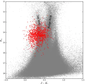
Fig. 2. Ksvs. (J−Ks) CMD of the complete catalog of RR Lyrae stars
(red stars) compared with the sources in tileb201as background. The CMD shows two prominent features, the disk main sequence (MS) and the bulge red giant branch (RGB), which are identified in the figure.
(Elorrieta et al., in prep.). We will use a similar classifier in
the near future to produce a catalog of VVV variable sources
classified using automated procedures (for more details see
Catelan et al. 2013b
;
Angeloni et al. 2014
).
One of the 28 tiles explored is obliterated by the presence of
a very bright star, resulting in fewer RR Lyrae discovered. Tile
b205
contains the star
η
Sgr (HD 167600), which is very bright
in the near-IR with
K
s∼ −1
.
55 mag. Such a bright star not only
saturates the detector, but also causes reflections that a
ff
ect the
flat fields; the resulting mosaic of this tile contains regions that
are not suitable for variability searches. This is the reason why
tile
b205
contains fewer RRab stars (
N
RRab=
31) than the rest
of the tiles (
N
RRab∼
37 on average).
Our RRab light curves have 60–62 data points with a median
magnitude of
K
s=
14
.
2 mag (12
.
1
.
K
s.
16
.
3). At this
mag-nitude level the completeness of the VVV source catalogues is
high, with about 95% detection e
ffi
ciency in less crowded fields
such as the outermost bulge region (
Saito et al. 2012a
). On the
other hand, experiments of signal detection rates based on VVV
data for RRab stars reach about 90% detection when applied to
light curves with 60 epochs (
Catelan et al. 2013b
). Therefore, we
can estimate the completeness of our RRab sample as accurately
as 80% for
K
s.
15 mag, with no expected trends along the two
axes, since crowding and extinction are similar across the
an-alyzed area. At fainter magnitudes the completeness is smaller
and makes it di
ffi
cult to find the most distant RR Lyrae, for
ex-ample the ones that may belong to the Sgr dwarf galaxy.
How-ever, we identify a few Sgr RR Lyrae candidates (see Sect.
3.1
).
We also checked the completeness of our catalogue by
comparing our findings with the RR Lyrae found by OGLE
in a small fraction of our area which overlaps an OGLE IV
field (
Soszy´nski et al. 2014
). There are 22 RR Lyrae stars with
−10
.
3
◦.
b
.
−8
.
0
◦in the OGLE IV catalog, of which we will
only focus on the 13 RRab stars present. In our catalog there
are eight matches within
d
<
1
00in tiles
b220
and
b221
. Three
of the five remaining RRab stars were not analyzed by our
al-gorithm owing to non-stellar photometry flags or fewer epochs
Fig. 3.Top panel: Bailey diagram of the complete RRab catalog. The OoI (solid) and OoII (dashed) lines derived byNavarrete et al.(2015) are shown. Bottom panel: period histogram of the 1019 RRab stars with bins adapted by the Bayesian Block algorithm (Scargle et al. 2013) through theastroMLimplementation (Vanderplas et al. 2012).
the last two RRab stars in the area in our catalog. With these
corrections our completeness with respect to the OGLE survey
is at least 80%. Certainly, not all of the RRab stars in the catalog
are new discoveries. We match our catalog with the General
Cat-alogue of Variable Stars (GCVS;
Samus et al. 2009
) and find a
total of 207 matches. VVV IDs and the respective GCVS names
for matching objects are presented in Appendix A. We note that
none of our classified RRab stars has tagged eclipsing binary
counterparts in the GCVS, even though we do not discard minor
contamination due to eclipsing binaries that can mimic RRab
stars. Finally, 27 of the RRab stars in the tile
b201
have already
een reported y
Gran et al.
(
2015
).
3. Results
After accounting for the duplicates, a total of 1019 RRab stars
remained in our sample. The final catalogue is presented in
Ap-pendix A. In the first step we characterized this sample in terms
of its calculated magnitude-weighted
h
K
si,
h
J
i − h
K
si
colour,
pe-riods, amplitudes, light curve shapes, and, coordinates. Figure
2
shows the
J
−
K
scolour–magnitude diagram (CMD) for the
com-plete RR Lyrae catalog with tile
b201
as a comparison field. The
RR Lyrae stars lie in a wide range of mean-
K
smagnitudes owing
to their distance distribution in the Galaxy, but the
J
−
K
scolour
is limited between
∼0.0 and 0.6, similar values to those reported
by
Gran et al.
(
2015
).
0.3 0.4 0.5 0.6 0.7 0.8 0.9 1.0
series (sine based) using the DFF routine.
diagram we can see that our RR Lyrae stars are predominantly
Oosterho
ff
Type I (OoI) with a minor composition of Oosterho
ff
Type II (OoII). We derived this composition with the Oosterhoof
reference lines traced by
Navarrete et al.
(
2015
).
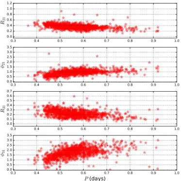
In addition to the period and amplitude, another
character-istic feature of the RRab stars is the light curve shape, which
can be described by a Fourier series. A sine decomposition up to
sixth order was performed with the direct Fourier fitting (DFF)
routine given by
Kovács & Kupi
(
2007
). Figure
4
shows the
R
21,
φ
21,
R
31, and
φ
31coe
ffi
cients as function of the period. All
the Fourier components tend to be clustered in a limited region
in this space (for reference see Fig. 6 of
Deb & Singh 2010
).
There were some outliers in the distributions (e.g.: RRab with
R
21>
0
.
6 or
φ
21>
2), which were visually inspected; some
gaps in the light curve were found that have an e
ff
ect on the final
value.
The spatial distribution in Galactic coordinates of the
cata-log is shown in Fig.
5
. The observations span only 2
◦in
b
, but
more than 20
◦in
`
, resulting in the very elongated shape of the
figure. Although there are no globular clusters in the analyzed
area according to the
Francis & Anderson
(
2014
) catalog, their
presence in nearby regions could bias the number of RR Lyrae
stars found. This possible e
ff
ect on our catalog was investigated
on the three closest globular clusters to our sample of RRab stars.
NGC 6656 is the only cluster that has associated RR Lyrae stars
according to
Clement et al.
(
2001
, 2015 editiononline catalog
2),
but the closest variable is 10
0further from the cluster tidal radius
(
rt
≈
30
0) given by the 2010 version of the
Harris
(
1996
)
cata-log. NGC 6624 and 6637 are considered metal-rich clusters with
[Fe
/
H] values of
−0
.
63 and
−0
.
77, respectively (
Valenti et al.
2004
,
2005
). Both clusters develop a very red horizontal branch,
which is the reason why they are not known to have associated
RR Lyrae stars.
2 http://www.astro.utoronto.ca/~cclement/read.html
3.1. Distances and the 3D view of the outer bulge
One of the main goals of the VVV Survey is to trace the
Galac-tic structure using variable stars in order to make the most
com-plete 3D view of the central regions of our Galaxy (
Minniti et al.
2010
). The primary distance indicators are the RR Lyrae stars
owing to the high number density present in the bulge area
(
Soszy´nski et al. 2014
) and the tight period–luminosity (P-L)
re-lation that they follow in near-IR bands (
Longmore et al. 1990
;
Catelan et al. 2004
). To obtain the distance values, first we must
calculate the reddening and extinction values to the individual
variables. The former can be obtained through the di
ff
erence
be-tween the mean-apparent and absolute magnitudes of our RRab
stars, given by
E
(
J
−
K
s)
=
(
J
−
K
s)
−
(
J
−
K
s)
0=
(
J
−
K
s)
−
(
MJ
−
MK
s)
,
(1)
where (
J
−
K
s)
0is the intrinsic colour of our RRab star and
M
Xthe absolute magnitude in the
X
-band. In our analysis we adopt
the P-L relations derived by
Alonso-García et al.
(
2015
) to
re-cover the absolute magnitudes of the RR Lyrae stars in the
J
- and
K
s-bands with log
Z
=
[Fe
/
H]
−1
.
765, based on a solar
metallic-ity of
Z
=
0
.
017 (
Catelan et al. 2004
). To calculate the
J
-band
mean magnitudes for the stars in our catalog we performed a
lin-ear regression between the
J
- and
K
s-band mean magnitudes of
the RRab stars of
ω
Centauri studied by Navarrete et al. (2016).
This analysis is needed because the VVV Survey only provides
one observation in the
ZY JH
-bands. The resulting fit is given by
h
J
i
=
0
.
93
× h
K
si
+
1
.
26. As expected, the residuals are
cen-tred in 0 with a dispersion of 0.03 mag. This allows us to derive
the reddening on a star-by-star basis, and also the extinction of
each RRab star by adopting an extinction law (e.g.
Cardelli et al.
1989
).
At this point we calculate the distances given by
log
d
=
1
+
0
.
2(
K
s,0−
MK
s)
,
(2)
with
d
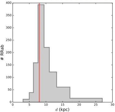
the individual distance in pc to our RRab stars. Figure
6
shows the distribution of distances of the RRab stars in our
cata-log. The vertical line corresponds to the Galactic centre distance
derived in
Dékány et al.
(
2013
) with a value of
R
0≈
8
.
33 kpc.
Our distances have a maximum frequency around
R
0where
the centre of the distribution is, and an asymmetric shape
to-wards the far side of the bulge because the volume observed is
greater owing to the cone e
ff
ect. According to their distances,
some of the RR Lyrae stars may belong to the Sagittarius dwarf
spheroidal (Sgr dSph) galaxy (e.g. distances around 20 kpc).
Kunder & Chaboyer
(
2009
) place the core of the Sgr dSph
galaxy at
∼22–27 kpc from the Sun, but
∼4
◦away from our
an-alyzed region. Even taking into account that Sgr RR Lyrae stars
are mixed with the Milky Way halo variables, some RR Lyrae
stars found towards these coordinates have been associated with
the dwarf galaxy by MACHO (
Alard 1996
;
Alcock et al. 1997
)
and OGLE (
Soszy´nski et al. 2014
).
The elongated shape of the analyzed area allows us to
ap-proximate the observation volume with a circular sector,
pro-jecting the
b
coordinate. Figure
7
shows distances and Galactic
longitude in this line-of-sight circular projection. The RR Lyrae
stars tend to stay near the projected Galactic centre distance
(
d
≈
8 kpc) and the previously mentioned Sgr dSph RR Lyrae
candidates are clearly visible in the 16
≤
d
(kpc)
≤
22 and
`
≥
6
◦zone.
3.2. To trace or not to trace: the X-shaped problem
Fig. 5.Spatial distribution in Galactic coordinates (`,b) of the RRab stars found in this work.
Fig. 6.Distribution of distances of the RR Lyrae stars found. The ver-tical line represents the Galactic centre derived byDékány et al.(2013) with OGLE-III RR Lyrae stars ofR0≈8.33 kpc.
are important distance indicators (e.g. RR Lyrae and Cepheids,
among others), but in addition to this method, the red clump
stars were also used in near-IR single-epoch studies to
de-rive accurate distances to the Milky Way edge (
Minniti et al.
2011
), bulge (
Alves 2000
), or the Large Magellanic Cloud
(
Alves et al. 2002
). This feature of the red clump stars has
been used recently to discover the X-shaped structure of
the Milky Way (
McWilliam & Zoccali 2010
;
Nataf et al. 2010
;
Saito et al. 2011
;
Wegg & Gerhard 2013
) that contains a bar at
its central (
Rattenbury et al. 2007
;
Gonzalez et al. 2011
). This
structure probably vanishes with decreasing metallicity of stars,
and it is not expected in an old stellar population (
Ness et al.
2012
). It is clear and well studied that the red clump stars
follow this barred Galactic feature, but in the RR Lyrae case
there is no clear evidence for the same trend. On the one hand
Pietrukowicz et al.
(
2012
) with OGLE-III RR Lyrae stars claim
the existence of the barred structure rotated about 30
◦with
re-spect to the line of sight between the Sun and the Galactic
cen-tre. On the other hand,
Dékány et al.
(
2013
) completely rule out
this possibility using the same dataset, but included the near-IR
results of the VVV Survey.
We used our catalogue to compare the distribution of
RR Lyrae at low Galactic latitude with the distribution of red
clump stars in the same analyzed tiles. Both catalogues were
di-vided into three longitude bins:
−10
◦< ` <
−3
.
5
◦;
−3
.
5
◦< ` <
3
.
5
◦; and 3
.
5
◦< ` <
10
◦. The red clump stars were selected with
the same technique described in
Minniti et al.
(
2011
) with
mag-at distances closer than
∼
20 kpc. The distributions of the red
clump stars also include the contribution of the underlying RGB.
The RGB does not change the position of the red clump, thus
the distributions are suitable for our comparison purposes.
As-suming an intrinsic red clump absolute magnitude
M
Ks=
−1
.
55
and an intrinsic red clump colour (
J
−
K
s)
0=
0
.
68, as given by
Gonzalez et al.
(
2011
) for Baade’s window red clump stars, the
distance equation yields
µ
=
−5
+
5 log
d
(pc)
=
K
s−
0
.
73(
J
−
K
s)
+
2
.
05
,
(3)
where the
Cardelli et al.
(
1989
) extinction law was assumed.
Figure
8
shows the result of the comparison between the
dis-tance distribution of red clump and RR Lyrae stars. The red
ver-tical line shows the mean distance value of a single-Gaussian
fit to the RR Lyrae in each longitude bin, namely
d
RRL∼
9
.
01,
8
.
63, and 8
.
98 kpc, from positive to negative longitudes,
respec-tively, with associated standard deviations of
σ
RRL∼
1
.
36, 1
.
31,
and 1.35. Clearly, the variation in the mean distance across the
longitude direction is negligible for the RR Lyrae distribution.
Red clump stars, on the contrary, show a single peak at
d
RC∼
6
.
8 kpc at positive longitudes, two peaks at
d
RC∼
6
.
8 and 9.5 kpc
across the minor axis, and a single peak at
d
RC∼
9
.
4 kpc at
neg-ative longitudes. In all three cases, a two-sample
Kolmogorov-Smirnov test reveals that the distributions of red clump and
RR Lyrae stars are indeed di
ff
erent, with higher than 98.9%
probability. This strongly suggests that the red clump stars (but
not the RR Lyrae) follow the main Galactic bar, flaring up into
a peanut shape (or X-shape) far away from the Galactic plane.
The marked di
ff
erence in the distance distribution of RR Lyrae
variables and red clump stars confirms at low latitudes the
con-clusion by
Dékány et al.
(
2013
) that RR Lyrae and RC stars trace
two di
ff
erent components in the bulge.
4. Summary
A search for RR Lyrae stars was performed in more than
∼47 sq deg in the outer parts of the Galactic bulge observed by
the VVV Survey. In total, more than 1000 fundamental mode
RR Lyrae stars were found in this area, with an estimated
com-pleteness level of 80% for
K
s≤
15 mag. We analyzed their
−
12
.
0
◦Fig. 7.Cone-view (d, `) of the analyzed area in the Galactic bulge. The sample is concentrated around the projection of the Galactic centre.
0 5 10 15 20 25
Fig. 8.Histogram of distances of RR Lyrae (filled) and red clump stars (steps) as function of Galactic latitude (`). The distributions of the red clump stars include also the underlying RGB, but since those do not affect the position of the red clump the distributions are suitable for our comparison purposes. The total number of red clump stars in the same areas overwhelms the number of RR Lyrae, thus the histogram showing their distribution in distance was normalized for better visualization. The vertical line represents the RR Lyrae mean distance of each region.
when fully automatic searches in the VVV Survey area is
com-pleted (
Catelan et al. 2013b
;
Angeloni et al. 2014
).
Acknowledgements. We gratefully acknowledge the use of data from the ESO Public Survey program ID 179.B-2002 taken with the VISTA telescope and data products from the Cambridge Astronomical Survey Unit. Support for the au-thors is provided by the BASAL CATA Center for Astrophysics and Associ-ated Technologies through grant PFB-06, and the Ministry for the Economy, De-velopment, and Tourism’s Programa Iniciativa Científica Milenio through grant IC120009, awarded to the Millennium Institute of Astrophysics (MAS). D.M. and M.Z. acknowledge support from FONDECYT Regular grants No. 1130196 and 1150345, respectively. Partial support for this project is provided by CON-ICYT’s PCI program through grant DPI20140066. F.G., C.N., and M.C. ac-knowledge support from FONDECYT regular grant No. 1141141. C.N. and F. G. acknowledge support from CONICYT-PCHA Doctorado and Magíster Na-cional 2015-21151643 and 2014-22141509, respectively. R.K.S. acknowledges support from CNPq/Brazil through projects 310636/2013-2 and 481468/2013-7. We gratefully acknowledge the use of IPython, Astropy, AstroML, Matplotlib, TOPCAT, and ALADIN sky atlas.
References
Alard, C. 1996,ApJ, 458, L17
Alcock, C., Allsman, R. A., Axelrod, T. S., et al. 1996,AJ, 111, 1146
Alcock, C., Allsman, R. A., Alves, D. R., et al. 1997,ApJ, 474, 217
Alonso-García, J., Dékány, I., Catelan, M., et al. 2015,AJ, 149, 99
Alves, D. R. 2000,ApJ, 539, 732
Alves, D. R., Rejkuba, M., Minniti, D., & Cook, K. H. 2002,ApJ, 573, L51
Angeloni, R., Contreras Ramos, R., Catelan, M., et al. 2014,A&A, 567, A100
Aubourg, E., Bareyre, P., Brehin, S., et al. 1993,The Messenger, 72, 20
Bailey, S. I. 1902,Annals of Harvard College Observatory, 38, 1
Benjamin, R. A., Churchwell, E., Babler, B. L., et al. 2005,ApJ, 630, L149
Cardelli, J. A., Clayton, G. C., & Mathis, J. S. 1989,ApJ, 345, 245
Carpenter, J. M., Hillenbrand, L. A., & Skrutskie, M. F. 2001,AJ, 121, 3160
Catelan, M., & Smith, H. A. 2015, Pulsating Stars (Wiley-VCH) Catelan, M., Pritzl, B. J., & Smith, H. A. 2004,ApJS, 154, 633
Catelan, M., Dekany, I., Hempel, M., & Minniti, D. 2013a, Boletin de la Asociacion Argentina de Astronomia La Plata Argentina, 56, 153
Catelan, M., Minniti, D., Lucas, P. W., et al. 2013b, in 40 Years of Variable Stars: A Celebration of Contributions by Horace A. Smith, eds. K. Kinemuchi et al.
[arXiv:1310.1996]
Clement, C. M., Muzzin, A., Dufton, Q., et al. 2001,AJ, 122, 2587
Deb, S., & Singh, H. P. 2010,MNRAS, 402, 691
Debosscher, J., Sarro, L. M., Aerts, C., et al. 2007,A&A, 475, 1159
Dékány, I., Minniti, D., Catelan, M., et al. 2013,ApJ, 776, L19
Dékány, I., Minniti, D., Hajdu, G., et al. 2015,ApJ, 799, L11
Francis, C., & Anderson, E. 2014,MNRAS, 441, 1105
Gonzalez, O. A., Rejkuba, M., Minniti, D., et al. 2011,A&A, 534, L14
Gonzalez, O. A., Rejkuba, M., Zoccali, M., et al. 2013,A&A, 552, A110
Gran, F., Minniti, D., Saito, R. K., et al. 2015,A&A, 575, A114
Harris, W. E. 1996,AJ, 112, 1487
Hempel, M., Minniti, D., Dékány, I., et al. 2014,The Messenger, 155, 29
Kovács, G., & Kupi, G. 2007,A&A, 462, 1007
Kunder, A., & Chaboyer, B. 2009,AJ, 137, 4478
Longmore, A. J., Dixon, R., Skillen, I., Jameson, R. F., & Fernley, J. A. 1990,
MNRAS, 247, 684
Lucas, P. W., Hoare, M. G., Longmore, A., et al. 2008,MNRAS, 391, 136
McWilliam, A., & Zoccali, M. 2010,ApJ, 724, 1491
Minniti, D., Lucas, P. W., Emerson, J. P., et al. 2010,New Astron., 15, 433
Minniti, D., Saito, R. K., Alonso-García, J., Lucas, P. W., & Hempel, M. 2011,
ApJ, 733, L43
Navarrete, C., Contreras Ramos, R., Catelan, M., et al. 2015,A&A, 577, A99
Navarrete, C., Catelan, M., Contreras Ramos, R., Gran, F. & Alonso-Garia, J. 2016,Communication from the Konkoly Observatory, 105, 45
Nataf, D. M., Udalski, A., Gould, A., Fouqué, P., & Stanek, K. Z. 2010,ApJ, 721, L28
Ness, M., Freeman, K., Athanassoula, E., et al. 2012,ApJ, 756, 22
Pietrukowicz, P., Udalski, A., Soszy´nski, I., et al. 2012,ApJ, 750, 169
Rattenbury, N. J., Mao, S., Sumi, T., & Smith, M. C. 2007,MNRAS, 378, 1064
Richards, J. W., Starr, D. L., Butler, N. R., et al. 2011,ApJ, 733, 10
Saito, R. K., Zoccali, M., McWilliam, A., et al. 2011,AJ, 142, 76
Saito, R. K., Hempel, M., Minniti, D., et al. 2012a,A&A, 537, A107
Saito, R. K., Minniti, D., Dias, B., et al. 2012b,A&A, 544, A147
Samus, N. N., & Durlevich, O. V. 2009, VizieR Online Data Catalog: B/gcvs Scargle, J. D., Norris, J. P., Jackson, B., & Chiang, J. 2013,ApJ, 764, 167
Schultheis, M., Chen, B. Q., Jiang, B. W., et al. 2014,A&A, 566, A120
Schwarzenberg-Czerny, A. 1989,MNRAS, 241, 153
Skrutskie, M. F., Cutri, R. M., Stiening, R., et al. 2006,AJ, 131, 1163
Soszy´nski, I., Udalski, A., Szyma´nski, M. K., et al. 2014,Acta Astron., 64, 177
Udalski, A., Szyma´nski, M. K., & Szyma´nski, G. 2015,Acta Astron., 65, 1
Valenti, E., Ferraro, F. R., & Origlia, L. 2004,MNRAS, 351, 1204
Valenti, E., Origlia, L., & Ferraro, F. R. 2005,MNRAS, 361, 272
Vanderplas, J., Connolly, A., Ivezi´c, Ž., & Gray, A. 2012, in Conf. on Intelligent Data Understanding (CIDU), 47
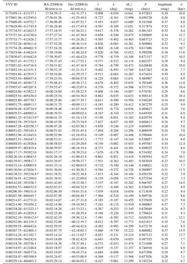
Appendix A: List of VVV RRab variables
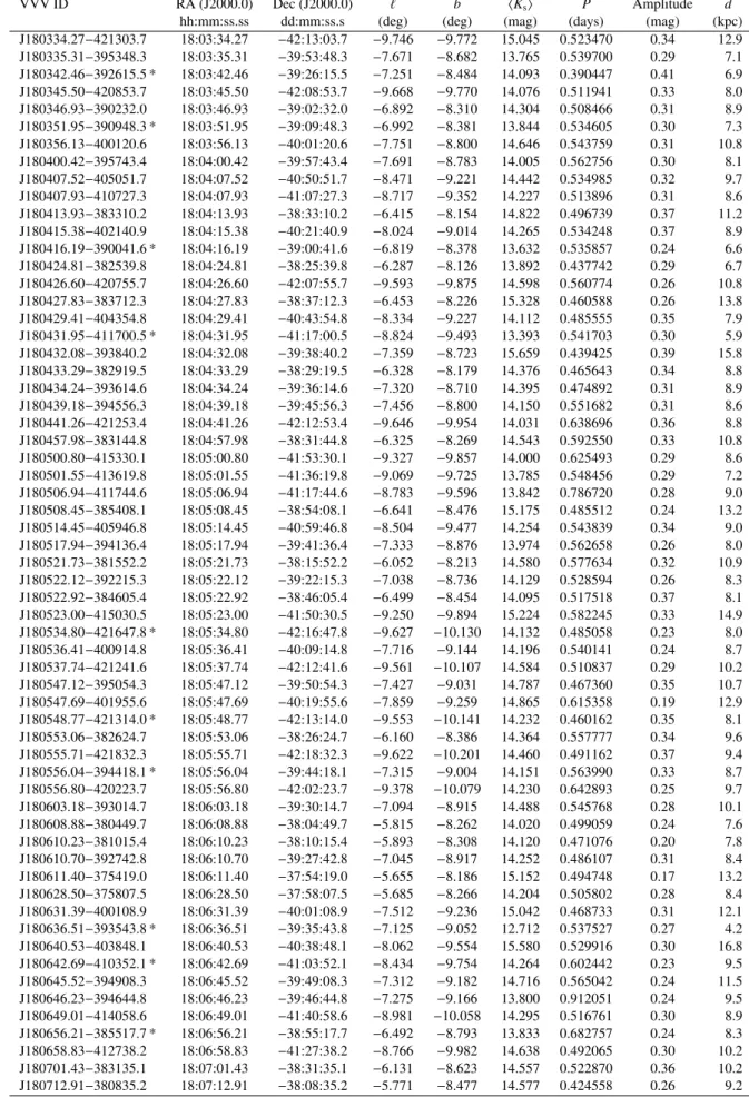
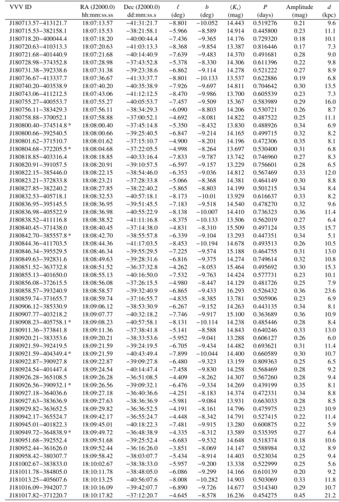
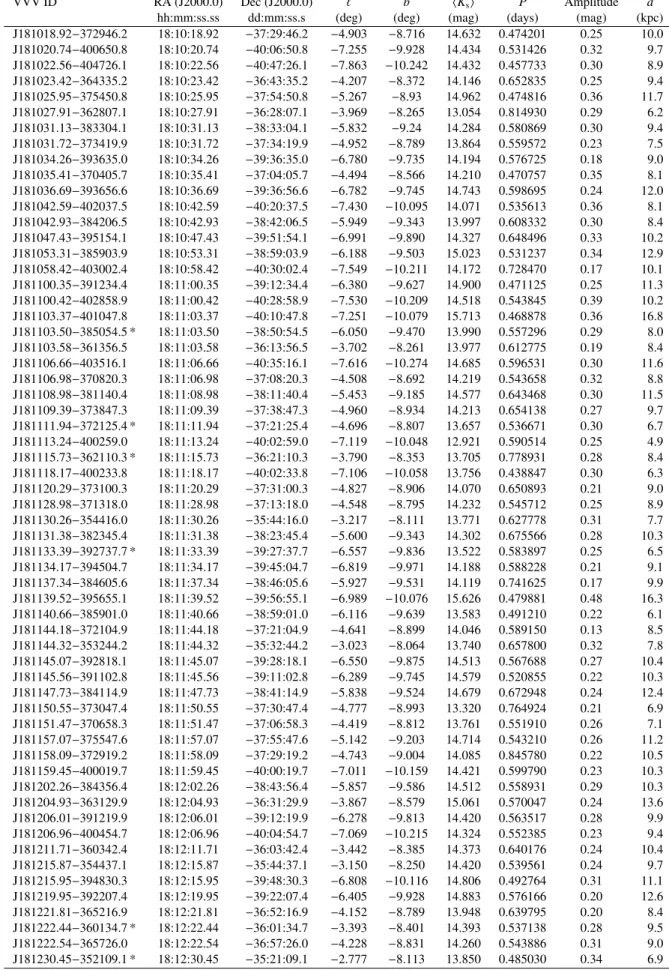
Table A.1 lists the main parameters of the 1019 ab-type RR Lyrae stars discovered in this work. For each object we provide the
VVV name, equatorial and Galactic coordinates, mean
K
s-band weighted-magnitude, period, amplitude, and heliocentric distance.
In Table A.2 we list the VVV RR Lyrae matching variables in the General Catalogue of Variable Stars (GCVS).
Table A.1.VVV RRab variables.
VVV ID RA (J2000.0) Dec (J2000.0) ` b hKsi P Amplitude d
hh:mm:ss.ss dd:mm:ss.s (deg) (deg) (mag) (days) (mag) (kpc)
J175459.11−413137.1 17:54:59.11 −41:31:37.1 −9.908 −8.039 14.641 0.472833 0.30 10.0
J175601.56−412549.0 17:56:01.56 −41:25:49.0 −9.727 −8.161 13.998 0.656728 0.26 8.8
J175609.49−410752.7 17:56:09.49 −41:07:52.7 −9.451 −8.037 14.009 0.541568 0.37 8.0
J175628.40−411745.8 17:56:28.40 −41:17:45.8 −9.567 −8.169 13.651 0.517874 0.32 6.5
J175718.55−412623.3 17:57:18.55 −41:26:23.3 −9.617 −8.376 14.262 0.481343 0.35 8.4
J175727.54−414338.0 17:57:27.54 −41:43:38.0 −9.858 −8.540 14.875 0.589605 0.34 12.7
J175733.77−412426.2 17:57:33.77 −41:24:26.2 −9.565 −8.402 14.465 0.683723 0.23 11.2
J175752.28−403611.6 17:57:52.28 −40:36:11.6 −8.826 −8.063 14.261 0.569084 0.32 9.2
J175754.28−404601.9 17:57:54.28 −40:46:01.9 −8.968 −8.148 14.476 0.617486 0.34 10.7
J175819.66−414624.9 17:58:19.66 −41:46:24.9 −9.820 −8.704 15.012 0.599208 0.38 13.6
J175830.07−414442.0 17:58:30.07 −41:44:42.0 −9.778 −8.719 14.348 0.671317 0.27 10.5
J175837.43−411752.1 17:58:37.43 −41:17:52.1 −9.371 −8.523 14.134 0.662357 0.28 9.4
J175851.82−414716.9 17:58:51.82 −41:47:16.9 −9.784 −8.799 14.473 0.628840 0.26 10.8
J175852.19−412131.5 17:58:52.19 −41:21:31.5 −9.402 −8.593 13.769 0.637263 0.26 7.7
J175854.86−412915.7 17:58:54.86 −41:29:15.7 −9.513 −8.663 14.283 0.474424 0.30 8.5
J175923.54−400457.8 17:59:23.54 −40:04:57.8 −8.224 −8.065 13.831 0.484907 0.32 6.9
J175948.43−403817.5 17:59:48.43 −40:38:17.5 −8.678 −8.402 15.035 0.392449 0.36 11.0
J175955.47−403207.4 17:59:55.47 −40:32:07.4 −8.576 −8.372 14.506 0.571716 0.30 10.4
J180024.80−415822.5 18:00:24.80 −41:58:22.5 −9.808 −9.140 14.087 0.578781 0.29 8.6
J180025.54−405436.0 18:00:25.54 −40:54:36.0 −8.862 −8.635 14.633 0.508143 0.28 10.4
J180025.80−403739.7 18:00:25.80 −40:37:39.7 −8.611 −8.500 14.594 0.548249 0.34 10.6
J180031.75−400913.3 18:00:31.75 −40:09:13.3 −8.181 −8.290 14.412 0.567270 0.25 9.9
J180038.48−410734.9 18:00:38.48 −41:07:34.9 −9.035 −8.774 14.036 0.489627 0.28 7.6
J180039.53−400902.4 18:00:39.53 −40:09:02.4 −8.167 −8.310 13.515 0.649705 0.31 6.9
J180041.35−411613.9 * 18:00:41.35 −41:16:13.9 −9.158 −8.851 14.182 0.629759 0.36 9.4
J180043.58−393334.9 18:00:43.58 −39:33:34.9 −7.637 −8.037 14.305 0.600413 0.34 9.7
J180047.28−420358.3 * 18:00:47.28 −42:03:58.3 −9.858 −9.246 13.219 0.604051 0.28 5.8
J180051.02−395145.4 18:00:51.02 −39:51:45.4 −7.894 −8.204 13.298 0.806959 0.24 7.0
J180052.96−411645.6 18:00:52.96 −41:16:45.6 −9.149 −8.887 14.448 0.598466 0.31 10.4
J180053.51−394347.3 18:00:53.51 −39:43:47.3 −7.772 −8.147 14.244 0.538057 0.34 8.9
J180058.03−412928.6 18:00:58.03 −41:29:28.6 −9.330 −9.002 15.033 0.495587 0.34 12.4
J180059.97−401819.4 18:00:59.97 −40:18:19.4 −8.273 −8.441 14.301 0.498925 0.33 8.8
J180117.17−393923.0 18:01:17.17 −39:39:23.0 −7.670 −8.178 13.988 0.534302 0.34 7.8
J180126.10−410043.4 18:01:26.10 −41:00:43.4 −8.861 −8.851 14.418 0.585954 0.27 10.1
J180129.07−395817.7 18:01:29.07 −39:58:17.7 −7.931 −8.363 14.493 0.583019 0.23 10.5
J180133.14−420003.9 18:01:33.14 −42:00:03.9 −9.732 −9.340 14.146 0.448021 0.32 7.7
J180136.04−415026.5 18:01:36.04 −41:50:26.5 −9.584 −9.272 14.728 0.560897 0.31 11.5
J180138.52−395238.8 * 18:01:38.52 −39:52:38.8 −7.833 −8.344 14.184 0.456159 0.22 7.9
J180138.91−412209.0 18:01:38.91 −41:22:09.0 −9.159 −9.056 13.779 0.572194 0.27 7.3
J180142.05−393258.3 18:01:42.05 −39:32:58.3 −7.537 −8.197 15.202 0.566707 0.27 14.5
J180203.53−400432.9 18:02:03.53 −40:04:32.9 −7.971 −8.509 14.503 0.526078 0.23 9.9
J180206.50−390151.6 18:02:06.50 −39:01:51.6 −7.039 −8.018 14.054 0.713638 0.22 9.4
J180207.98−400449.7 18:02:07.98 −40:04:49.7 −7.968 −8.524 14.109 0.569726 0.25 8.6
J180214.87−412731.0 18:02:14.87 −41:27:31.0 −9.185 −9.197 14.455 0.535828 0.27 9.8
J180214.90−391059.2 18:02:14.90 −39:10:59.2 −7.161 −8.115 13.910 0.500065 0.27 7.3
J180218.28−413322.1 * 18:02:18.28 −41:33:22.1 −9.267 −9.253 13.345 0.678049 0.24 6.5
J180222.40−412829.4 18:02:22.40 −41:28:29.4 −9.188 −9.226 13.970 0.756624 0.31 9.3
J180242.19−393612.4 * 18:02:42.19 −39:36:12.4 −7.491 −8.393 14.712 0.628354 0.31 12.1
J180252.00−401219.3 18:02:52.00 −40:12:19.3 −8.012 −8.707 13.773 0.621813 0.35 7.6
J180259.55−404442.6 18:02:59.55 −40:44:42.6 −8.482 −8.983 14.299 0.472170 0.42 8.5
J180307.75−421805.3 18:03:07.75 −42:18:05.3 −9.860 −9.739 15.222 0.660982 0.37 15.9
J180314.24−411102.7 18:03:14.24 −41:11:02.7 −8.851 −9.231 15.214 0.507123 0.32 13.7
J180318.09−384242.0 18:03:18.09 −38:42:42.0 −6.643 −8.070 14.053 0.487555 0.29 7.7
J180318.38−383758.1 18:03:18.38 −38:37:58.1 −6.573 −8.033 13.474 0.711698 0.27 7.1
J180318.97−412248.6 18:03:18.97 −41:22:48.6 −9.019 −9.337 13.357 0.746910 0.24 6.9
J180319.85−384537.6 18:03:19.85 −38:45:37.6 −6.684 −8.098 13.943 0.671998 0.29 8.7
J180324.07−405300.9 18:03:24.07 −40:53:00.9 −8.568 −9.117 13.568 0.657026 0.28 7.1
J180329.14−404403.2 18:03:29.14 −40:44:03.2 −8.427 −9.061 13.299 0.745234 0.32 6.7
Table A.1.continued.
VVV ID RA (J2000.0) Dec (J2000.0) ` b hKsi P Amplitude d
hh:mm:ss.ss dd:mm:ss.s (deg) (deg) (mag) (days) (mag) (kpc)
Table A.1.continued.
VVV ID RA (J2000.0) Dec (J2000.0) ` b hKsi P Amplitude d
hh:mm:ss.ss dd:mm:ss.s (deg) (deg) (mag) (days) (mag) (kpc)
Table A.1.continued.
VVV ID RA (J2000.0) Dec (J2000.0) ` b hKsi P Amplitude d
hh:mm:ss.ss dd:mm:ss.s (deg) (deg) (mag) (days) (mag) (kpc)
Table A.1.continued.
VVV ID RA (J2000.0) Dec (J2000.0) ` b hKsi P Amplitude d
hh:mm:ss.ss dd:mm:ss.s (deg) (deg) (mag) (days) (mag) (kpc)
Table A.1.continued.
VVV ID RA (J2000.0) Dec (J2000.0) ` b hKsi P Amplitude d
hh:mm:ss.ss dd:mm:ss.s (deg) (deg) (mag) (days) (mag) (kpc)
Table A.1.continued.
VVV ID RA (J2000.0) Dec (J2000.0) ` b hKsi P Amplitude d
hh:mm:ss.ss dd:mm:ss.s (deg) (deg) (mag) (days) (mag) (kpc)
J181713.34−372529.4 18:17:13.34 −37:25:29.4 −4.205 −9.903 14.074 0.611086 0.16 8.8 J181718.08−375812.6 18:17:18.08 −37:58:12.6 −4.693 −10.162 14.277 0.577264 0.33 9.4 J181723.79−371424.2 18:17:23.79 −37:14:24.2 −4.022 −9.851 14.357 0.520143 0.32 9.2 J181724.11−371520.9 18:17:24.11 −37:15:20.9 −4.035 −9.859 14.776 0.556967 0.29 11.7 J181724.66−345352.6 18:17:24.66 −34:53:52.6 −1.903 −8.795 14.332 0.462888 0.29 8.5 J181725.42−334742.4 * 18:17:25.42 −33:47:42.4 −0.909 −8.295 13.950 0.534068 0.20 7.7 J181726.05−361312.1 * 18:17:26.05 −36:13:12.1 −3.094 −9.398 13.709 0.707879 0.30 7.9 J181727.29−335532.1 ** 18:17:27.29 −33:55:32.1 −1.024 −8.360 13.612 0.675320 0.20 7.4 J181727.55−354403.3 * 18:17:27.55 −35:44:03.3 −2.653 −9.183 14.252 0.623970 0.30 9.7 J181733.97−353109.9 * 18:17:33.97 −35:31:09.9 −2.449 −9.105 14.094 0.602439 0.33 8.8 J181742.23−344836.6 * 18:17:42.23 −34:48:36.6 −1.796 −8.809 12.531 0.619138 0.35 4.2 J181745.11−333025.2 ** 18:17:45.11 −33:30:25.2 −0.619 −8.224 14.951 0.505283 0.30 12.1 J181745.70−333214.2 * 18:17:45.70 −33:32:14.2 −0.645 −8.239 14.915 0.440511 0.24 11.0 J181746.66−335654.5 * 18:17:46.66 −33:56:54.5 −1.013 −8.430 13.849 0.567769 0.27 7.5 J181747.66−342504.7 18:17:47.66 −34:25:04.7 −1.434 −8.647 14.181 0.623088 0.31 9.3 J181749.89−335146.2 * 18:17:49.89 −33:51:46.2 −0.931 −8.401 14.726 0.686168 0.31 12.8 J181749.93−344116.0 18:17:49.93 −34:41:16.0 −1.674 −8.776 14.168 0.531098 0.24 8.5 J181750.90−360357.6 * 18:17:50.90 −36:03:57.6 −2.917 −9.403 15.054 0.405131 0.30 11.3 J181752.16−372251.6 * 18:17:52.16 −37:22:51.6 −4.107 −9.998 14.290 0.450187 0.27 8.2 J181752.57−354131.3 18:17:52.57 −35:41:31.3 −2.576 −9.240 15.398 0.452464 0.40 14.1 J181752.60−331543.8 18:17:52.60 −33:15:43.8 −0.387 −8.135 14.912 0.468960 0.24 11.4 J181802.62−374619.9 18:18:02.62 −37:46:19.9 −4.446 −10.204 14.031 0.552614 0.28 8.1 J181805.35−325841.8 18:18:05.35 −32:58:41.8 −0.111 −8.045 14.522 0.593349 0.41 10.7 J181805.66−363810.4 * 18:18:05.66 −36:38:10.4 −3.411 −9.704 14.522 0.574538 0.28 10.5 J181806.34−370306.8 18:18:06.34 −37:03:06.8 −3.787 −9.893 13.694 0.596986 0.26 7.2 J181807.82−361359.6 * 18:18:07.82 −36:13:59.6 −3.042 −9.530 13.803 0.452860 0.38 6.5 J181808.39−341844.2 * 18:18:08.39 −34:18:44.2 −1.306 −8.662 13.006 0.643832 0.33 5.4 J181809.19−352945.0 18:18:09.19 −35:29:45.0 −2.373 −9.201 14.424 0.569671 0.31 10.0 J181810.15−373707.4 18:18:10.15 −37:37:07.4 −4.296 −10.158 14.581 0.571327 0.31 10.8 J181811.59−350633.2 * 18:18:11.59 −35:06:33.2 −2.020 −9.034 14.707 0.473711 0.34 10.4 J181812.84−351121.0 18:18:12.84 −35:11:21.0 −2.090 −9.073 13.648 0.615635 0.20 7.2 J181812.89−372939.2 18:18:12.89 −37:29:39.2 −4.178 −10.110 15.892 0.554961 0.34 20.0 J181814.52−325645.4 * 18:18:14.52 −32:56:45.4 −0.067 −8.059 14.226 0.464313 0.28 8.1 J181817.14−361754.9 * 18:18:17.14 −36:17:54.9 −3.087 −9.587 14.724 0.480716 0.33 10.5 J181819.94−363905.2 18:18:19.94 −36:39:05.2 −3.403 −9.754 13.326 0.656439 0.25 6.3 J181820.31−363721.3 18:18:20.31 −36:37:21.3 −3.376 −9.742 13.853 0.693900 0.25 8.4 J181824.70−363713.1 * 18:18:24.70 −36:37:13.1 −3.367 −9.754 13.962 0.619276 0.34 8.4 J181825.62−374652.8 18:18:25.62 −37:46:52.8 −4.420 −10.276 13.132 0.509510 0.30 5.0 J181826.01−363824.1 18:18:26.01 −36:38:24.1 −3.383 −9.767 13.506 0.607478 0.20 6.6 J181829.96−335611.7 18:18:29.96 −33:56:11.7 −0.934 −8.558 14.001 0.616835 0.27 8.5 J181831.18−341728.6 18:18:31.18 −34:17:28.6 −1.251 −8.723 13.866 0.565563 0.25 7.6 J181832.29−333757.2 18:18:32.29 −33:37:57.2 −0.656 −8.427 14.107 0.599797 0.27 8.8 J181833.18−350456.0 18:18:33.18 −35:04:56.0 −1.962 −9.087 13.805 0.527582 0.22 7.1 J181838.33−351351.3 * 18:18:38.33 −35:13:51.3 −2.088 −9.170 14.339 0.686243 0.32 10.6 J181843.83−335631.3 18:18:43.83 −33:56:31.3 −0.917 −8.603 13.477 0.570402 0.28 6.3
J181845.54−324431.1 18:18:45.54 −32:44:31.1 0.166 −8.062 13.791 0.629378 0.22 7.8
J181851.35−330614.5 18:18:51.35 −33:06:14.5 −0.150 −8.245 13.260 0.516041 0.28 5.4 J181852.52−344107.2 * 18:18:52.52 −34:41:07.2 −1.573 −8.967 13.954 0.576515 0.26 8.0 J181857.42−330033.9 * 18:18:57.42 −33:00:33.9 −0.055 −8.221 14.048 0.528505 0.29 8.0 J181903.62−351425.7 18:19:03.62 −35:14:25.7 −2.058 −9.251 15.040 0.813829 0.19 16.3 J181908.93−335354.1 * 18:19:08.93 −33:53:54.1 −0.837 −8.661 14.543 0.479322 0.32 9.6 J181910.10−331205.4 18:19:10.10 −33:12:05.4 −0.208 −8.348 14.071 0.493905 0.25 7.8 J181910.91−330421.6 * 18:19:10.91 −33:04:21.6 −0.090 −8.292 13.811 0.510326 0.31 7.0 J181913.13−353545.5 18:19:13.13 −35:35:45.5 −2.365 −9.440 13.762 0.572931 0.27 7.3 J181916.58−354855.4 * 18:19:16.58 −35:48:55.4 −2.558 −9.549 14.723 0.553814 0.38 11.4 J181917.03−331351.5 * 18:19:17.03 −33:13:51.5 −0.223 −8.383 14.682 0.468064 0.36 10.2 J181917.76−361647.4 * 18:19:17.76 −36:16:47.4 −2.977 −9.760 13.537 0.607648 0.33 6.7 J181918.16−365404.2 18:19:18.16 −36:54:04.2 −3.541 −10.039 14.325 0.490595 0.30 8.8 J181919.44−363429.4 * 18:19:19.44 −36:34:29.4 −3.243 −9.897 14.314 0.496934 0.34 8.8
Table A.1.continued.
VVV ID RA (J2000.0) Dec (J2000.0) ` b hKsi P Amplitude d
hh:mm:ss.ss dd:mm:ss.s (deg) (deg) (mag) (days) (mag) (kpc)
Table A.1.continued.
VVV ID RA (J2000.0) Dec (J2000.0) ` b hKsi P Amplitude d
hh:mm:ss.ss dd:mm:ss.s (deg) (deg) (mag) (days) (mag) (kpc)
Table A.1.continued
VVV ID RA (J2000.0) Dec (J2000.0) ` b hKsi P Amplitude d
hh:mm:ss.ss dd:mm:ss.s (deg) (deg) (mag) (days) (mag) (kpc)
Table A.1.continued.
VVV ID RA (J2000.0) Dec (J2000.0) ` b hKsi P Amplitude d
hh:mm:ss.ss dd:mm:ss.s (deg) (deg) (mag) (days) (mag) (kpc)
Table A.1.continued.
VVV ID RA (J2000.0) Dec (J2000.0) ` b hKsi P Amplitude d
hh:mm:ss.ss dd:mm:ss.s (deg) (deg) (mag) (days) (mag) (kpc)
Table A.1.continued.
VVV ID RA (J2000.0) Dec (J2000.0) ` b hKsi P Amplitude d
hh:mm:ss.ss dd:mm:ss.s (deg) (deg) (mag) (days) (mag) (kpc)
Table A.1.continued.
VVV ID RA (J2000.0) Dec (J2000.0) ` b hKsi P Amplitude d
hh:mm:ss.ss dd:mm:ss.s (deg) (deg) (mag) (days) (mag) (kpc)
Table A.1.continued.
VVV ID RA (J2000.0) Dec (J2000.0) ` b hKsi P Amplitude d
hh:mm:ss.ss dd:mm:ss.s (deg) (deg) (mag) (days) (mag) (kpc)
Table A.1.continued.
VVV ID RA (J2000.0) Dec (J2000.0) ` b hKsi P Amplitude d
hh:mm:ss.ss dd:mm:ss.s (deg) (deg) (mag) (days) (mag) (kpc)
Table A.1.continued.
VVV ID RA (J2000.0) Dec (J2000.0) ` b hKsi P Amplitude d
hh:mm:ss.ss dd:mm:ss.s (deg) (deg) (mag) (days) (mag) (kpc)
Table A.2.207 VVV RRab matching a variable in the General Cataloge of Variable Stars (GCVS).
| VVV ID GCVS name | VVV ID GCVS name |VVV ID GCVS name
| J2701020.22−411613.9 V0462 CrA | J2741313.37−375727.9 IP CrA |J2755443.71−341148.1 V2539 Sgr
| J2701149.18−420358.3 V0463 CrA | J2741423.44−381809.1 V0536 CrA |J2755521.67−312549.7 V3212 Sgr
| J2702437.84−395238.8 LM CrA | J2741507.38−341727.9 V2874 Sgr |J2755625.55−315420.3 V3216 Sgr
| J2703434.23−413322.1 V0469 CrA | J2741640.08−341613.8 V2878 Sgr |J2755732.00−335639.4 V3213 Sgr
| J2704032.86−393612.4 LT CrA | J2742121.33−334742.4 V2896 Sgr |J2755903.99−320723.9 V2540 Sgr
| J2705536.91−392615.5 MV CrA | J2742130.69−361312.1 V2889 Sgr |J2760118.99−313547.9 V3232 Sgr
| J2705759.29−390948.3 MY CrA | J2742153.30−354403.3 V2890 Sgr |J2760406.80−325426.8 V3242 Sgr
| J2710402.86−390041.6 NR CrA | J2742329.54−353109.9 V2899 Sgr |J2760436.45−343055.4 V3237 Sgr
| J2710759.32−411700.5 V0482 CrA | J2742533.40−344836.6 V0715 Sgr |J2760556.25−323912.0 V3248 Sgr
| J2712342.04−421647.8 V0483 CrA | J2742625.55−333214.2 V2914 Sgr |J2760606.68−341657.6 V3244 Sgr
| J2712711.57−421314.0 V0486 CrA | J2742639.96−335654.5 V2912 Sgr |J2760655.55−315252.5 V3253 Sgr
| J2712900.58−394418.1 OS CrA | J2742728.37−335146.2 V2920 Sgr |J2761027.42−324524.7 V3258 Sgr
| J2713907.68−393543.8 OX CrA | J2742743.43−360357.6 V2910 Sgr |J2761128.83−320258.6 V3243 Sgr
| J2714040.42−410352.1 V0398 CrA | J2742802.34−372251.6 IQ CrA |J2761405.62−344158.5 V2541 Sgr
| J2714403.10−385517.7 V0399 CrA | J2743124.89−363810.4 V2930 Sgr |J2761706.92−310451.3 V3287 Sgr
| J2720006.03−374514.8 GK CrA | J2743157.25−361359.6 V2933 Sgr |J2761732.22−332547.6 V3281 Sgr
| J2720110.20−372205.5 GO CrA | J2743205.87−341844.2 V2514 Sgr |J2762038.45−333047.8 V3292 Sgr
| J2721040.55−385557.8 PY CrA | J2743253.79−350633.2 V2938 Sgr |J2762108.32−305632.3 V3301 Sgr
| J2721703.45−405758.1 V0499 CrA | J2743337.74−325645.4 V2516 Sgr |J2762158.12−333306.2 V3298 Sgr
| J2722023.79−404349.4 QV CrA | J2743417.14−361754.9 V2941 Sgr |J2762248.05−305030.6 V3304 Sgr
| J2722138.38−390932.1 QX CrA | J2743610.45−363713.1 V2950 Sgr |J2762300.12−300107.2 V1606 Sgr
| J2722725.85−364838.9 V0636 Sgr | J2743934.92−351351.3 V2967 Sgr |J2762312.42−305056.7 V3306 Sgr
| J2724552.44−385054.5 V0506 CrA | J2744307.84−344107.2 V2978 Sgr |J2762441.01−310836.5 V3309 Sgr
| J2724759.12−372125.4 HN CrA | J2744421.33−330033.9 V2990 Sgr |J2762515.00−314838.5 V3310 Sgr
| J2724855.95−362110.3 V0650 Sgr | J2744713.95−335354.1 V2995 Sgr |J2762704.57−313947.8 V1607 Sgr
| J2725320.81−392737.7 V0344 CrA | J2744743.71−330421.6 V3010 Sgr |J2762905.51−320926.8 V2545 Sgr
| J2730536.57−360134.7 V2632 Sgr | J2744908.67−354855.4 V3000 Sgr |J2762939.84−333527.9 V3317 Sgr
| J2730736.80−352109.1 V2635 Sgr | J2744915.47−331351.5 V3015 Sgr |J2763120.75−321939.7 V3320 Sgr
| J2730922.26−350757.4 V2639 Sgr | J2744926.42−361647.4 V3001 Sgr |J2763156.71−312211.2 V3323 Sgr
| J2731008.91−364330.2 V2637 Sgr | J2744951.66−363429.4 V3004 Sgr |J2763530.59−342942.5 V3327 Sgr
| J2731133.29−352457.1 V0666 Sgr | J2745055.55−352208.4 V3016 Sgr |J2763657.89−332124.7 V3330 Sgr
| J2731501.17−362149.5 V0667 Sgr | J2745144.30−345327.4 V2519 Sgr |J2763804.58−314222.7 V3336 Sgr
| J2731638.55−354528.3 V2663 Sgr | J2750154.72−344558.4 V3053 Sgr |J2764121.09−314838.8 V3344 Sgr
| J2732239.38−354714.7 V2686 Sgr | J2750300.47−354837.4 V2523 Sgr |J2764232.11−310954.7 V3346 Sgr
| J2732624.49−375455.2 HU CrA | J2750422.74−352722.1 V3060 Sgr |J2764936.45−285937.0 V1302 Sgr
| J2732728.37−392931.4 V0355 CrA | J2750922.26−335458.0 V1186 Sgr |J2765058.13−321408.8 V3357 Sgr
| J2732809.37−361430.8 V0677 Sgr | J2750941.96−341525.6 V3078 Sgr |J2765205.63−334444.1 V3358 Sgr
| J2732945.94−363846.1 V0678 Sgr | J2751318.41−355135.9 V3090 Sgr |J2765316.64−322845.3 V2550 Sgr
| J2733036.67−363624.9 V3906 Sgr | J2751357.07−335539.8 V3093 Sgr |J2765317.11−331057.0 V3364 Sgr
| J2733048.87−380355.7 HX CrA | J2751532.70−334829.5 V1597 Sgr |J2765711.13−333149.7 V3372 Sgr
| J2733347.46−345714.6 V2727 Sgr | J2751657.42−335646.1 V1598 Sgr |J2770024.84−331118.4 V3377 Sgr
| J2733444.42−352242.8 V2728 Sgr | J2751727.49−364205.6 V3096 Sgr |J2770608.32−291328.3 V2555 Sgr
| J2733638.45−351449.5 V2734 Sgr | J2751751.21−314347.1 V3109 Sgr |J2770710.90−330519.7 V2554 Sgr
| J2733824.84−355455.0 V2739 Sgr | J2752229.17−321151.5 V1600 Sgr |J2770759.88−311120.0 V3399 Sgr
| J2733840.20−345906.3 V2744 Sgr | J2752614.30−340940.9 V1859 Sgr |J2770948.40−322348.4 V3402 Sgr
| J2734127.19−352035.6 V2753 Sgr | J2752744.07−313614.3 V1291 Sgr |J2771305.28−323916.3 V3410 Sgr
| J2734129.53−362705.8 V2748 Sgr | J2752752.85−340554.6 V3140 Sgr |J2771320.04−312151.2 V3414 Sgr
| J2734436.09−351324.8 V2758 Sgr | J2752826.49−342410.7 V3141 Sgr |J2771327.30−325251.9 V1611 Sgr
| J2734637.38−345411.4 V2770 Sgr | J2753005.28−322139.1 V3150 Sgr |J2771618.16−312636.2 V3419 Sgr
| J2734659.51−364323.7 V2767 Sgr | J2753217.00−340440.9 V3152 Sgr |J2772302.34−300956.8 V2564 Sgr
| J2734735.04−382330.9 V0364 CrA | J2753226.84−321623.3 V3153 Sgr |J2772755.20−310506.1 V2566 Sgr
| J2734959.70−365402.8 V0694 Sgr | J2753305.16−343822.8 V1292 Sgr |J2772830.47−310517.6 V2567 Sgr
| J2735029.17−344201.2 V2780 Sgr | J2753458.47−321936.8 V3162 Sgr |J2773243.47−323112.6 V3456 Sgr
| J2735217.92−360538.7 V0695 Sgr | J2753615.82−310753.9 V2535 Sgr |J2773409.84−283514.5 V1620 Sgr
| J2735345.71−344202.4 V0696 Sgr | J2753746.29−312237.5 V3169 Sgr |J2773624.61−305556.1 V3468 Sgr
| J2735602.11−372806.6 XX CrA | J2753937.74−333105.5 V3170 Sgr |J2773653.55−300103.9 V1621 Sgr
| J2735942.07−352754.8 V2806 Sgr | J2753946.75−311226.6 V3173 Sgr |J2774119.92−322237.8 V2355 Sgr
| J2740129.76−382259.4 V0533 CrA | J2754046.99−315352.7 V3174 Sgr |J2774210.91−310954.4 V3477 Sgr
| J2740343.90−364712.9 V2821 Sgr | J2754118.51−360331.8 V3168 Sgr |J2774605.04−321729.7 V3484 Sgr
| J2740423.85−365626.5 V0700 Sgr | J2754257.08−313412.0 V3178 Sgr |J2774758.36−314114.2 V3489 Sgr
Table A.2.continued.
| VVV ID GCVS name | VVV ID GCVS name |VVV ID GCVS name
| J2740455.20−353803.8 V0702 Sgr | J2754533.05−335723.9 V3180 Sgr |J2774809.03−314441.3 V3490 Sgr
| J2740715.58−351629.9 V0706 Sgr | J2754558.25−320110.0 V3188 Sgr |J2775727.88−311535.4 V2574 Sgr
| J2740722.74−352507.5 V0707 Sgr | J2754619.69−343303.0 V3183 Sgr |J2780805.50−310924.2 V1625 Sgr
| J2740748.40−351726.8 V0708 Sgr | J2754708.67−341138.0 V3186 Sgr |J2780843.71−312018.5 V2582 Sgr
| J2740804.45−334141.8 V2844 Sgr | J2754826.49−341617.6 V1295 Sgr |J2781001.76−313547.4 V2583 Sgr
| J2741013.01−354614.0 V2846 Sgr | J2754847.92−314745.3 V3193 Sgr |J2781358.59−312612.9 V3539 Sgr
| J2741048.75−340122.3 V2852 Sgr | J2754919.80−325428.2 V3191 Sgr |J2791305.39−291045.1 V2597 Sgr
| J2741123.21−333359.5 V2859 Sgr | J2754928.83−311656.0 V3197 Sgr |J2792632.46−281530.6 V1201 Sgr