Credit, liquidity and housing prices

Texto completo

(1)CREDIT, LIQUIDITY AND HOUSING PRICES. Author: Raúl Izquierdo Culebras.. 4th Course. Degree in Economics (2018/2019).. Contact e-mail: [email protected] Tutor: Juan Carlos Cuestas Olivares.. Abstract.. The document analyses links between real estate prices, interest rates, the amount of credit granted, the international direct investment position and the net income derived from tourism during the period between 2003 and 2016 for the Spanish case. For statistical evaluation, an autoregressive vectors model with quarterly frequency and four lags is used. The results highlight the net foreign direct investment position as the main factor, followed by interest rates and the credit granted divided by per capita income. Another determining factor is the autoregressive behavior shown by prices. There is practically no influence from tourism. It is necessary to emphasize the presence of wide confidence intervals in the impulse response functions that could compromise some of the results obtained.. Key words: Mortgages, interest rates, international investment, housing prices, bubble. JEL classification: A22, C51, E51, F36, G15, O52.

(2) Index.. 1.- Introduction............................................................................................................ 6 2.- Theoretical justification. ........................................................................................ 8 3.- Time series. .......................................................................................................... 14 4.- Econometric model. ............................................................................................ 21 4.1.- Necessary modifications. ............................................................................. 21 4.2.- Time series statistical analysis. ................................................................... 23 4.3.- Lag-order selection. ...................................................................................... 24 4.4.- Model formulation. ........................................................................................ 25 4.5.- Impulse Response functions. ....................................................................... 27 4.6.- Variance decomposition. .............................................................................. 33 5.- Conclusion ........................................................................................................... 35 6.- Appendices. ......................................................................................................... 37 7.- References. .......................................................................................................... 48 8.- Bibliography. ........................................................................................................ 49 9.- Database sources. ............................................................................................... 50. 2.

(3) Figure Index.. Figure 1: Evolution of price per square meter of houses more than 5 years old in Spain. ......................................................................................................................... 14 Figure 2: Evolution of the variations in the prices per square meter of houses more than 5 years old in Spain............................................................................................. 15 Figure 3: Evolution of mortgage interest rates over three years for Spain. ................. 16 Figure 4: Evolution of variations in mortgage interest rates over three years for Spain.. ................................................................................................................................... 16 Figure 5: Evolution of the monetary amount granted through mortgages divided by GDP per capita for Spain. ........................................................................................... 17 Figure 6: Evolution of the variations in the monetary amount granted through mortgages divided by GDP per capita for Spain. ......................................................... 18 Figure 7: Evolution of the net international investment position for Spain. .................. 18 Figure 8: Evolution of the variations in the net international investment position for Spain. ......................................................................................................................... 19 Figure 9: Evolution of net income from international tourism for Spain. ...................... 20 Figure 10: Evolution of variations in net income from international tourism for Spain. 20 Figure 11: Evolution of seasonally adjusted variations in net income from international tourism in Spain. ......................................................................................................... 22 Figure 12: Evolution of seasonally adjusted variations in the monetary amount granted through mortgages divided by GDP per capita for Spain. ............................................ 22 Figure 13: Seasonal component of variations in net income from international tourism for Spain. .................................................................................................................... 22 Figure 14: Seasonal component of variations in the monetary amount granted through mortgages divided by GDP per capita for Spain. ......................................................... 23 Figure 15: Response impulse functions with generalized orthogonal shocks. ............ 29 Figure 16: Response impulse functions with orthogonal Cholensky shocks for the first order proposed. .......................................................................................................... 31 Figure 17: Response impulse functions with orthogonal Cholensky shocks for the second order proposed. .............................................................................................. 32 Figure 18: Variance decomposition of the housing price prediction errors. ................. 33 Figure 19: Rest of impulse response functions with generalized orthogonal shocks... 42 Figure 20: Response impulse functions with generalized orthogonal shocks and accumulated responses. ............................................................................................. 43. 3.

(4) Figure 21: Rest of impulse response functions with orthogonal Cholensky shocks for the first order proposed ............................................................................................... 44 Figure 22: Response impulse functions with orthogonal Cholensky shocks and accumulated responses for the first proposed order.................................................... 45 Figure 23: Response impulse functions with orthogonal Cholensky shocks and accumulated responses for the second proposed order. ............................................. 46 Figure 24: Rest of error variance decomposition functions. ........................................ 47. 4.

(5) Table Index.. Table 1: Individual statistics of the series group used.. ............................................... 23 Table 2: Correlation matrix of the series used.. .......................................................... 24 Table 3: VAR lag order selection criteria. ................................................................... 25 Table 4: Seasonality test on evolution of variations in the net income derived from international tourism.................................................................................................... 37 Table 5: Seasonality test on evolution of variations in the monetary amount granted through mortgages divided by GDP per capita for Spain. ............................................ 37 Table 6: Seasonality test on evolution of the variations in the prices per square meter of houses more than 5 years old in Spain. ................................................................ 37 Table 7: Seasonality test on the evolution of variations in mortgage interest rates over three years for Spain................................................................................................... 37 Table 8: Seasonality test on the evolution of variations in the net international investment position for Spain. ..................................................................................... 38 Table 9: VAR Residual Correlation LM Tests for 3 lags. ............................................. 38 Table 10: VAR Residual Correlation LM Tests for 4 lags. ........................................... 39 Table 11: Vector autoregression estimates. ............................................................... 41. 5.

(6) 1.- Introduction.. The markets in recent decades have experienced inflationary processes which have sometimes resulted in serious bubbles. On the one hand, these trends have possibly been motivated by the excessive liquidity injection, increases in international trade, alterations in domestic supply and demand for goods and services or even associated with the excessive deregulation of the U.S. financial markets which encourage speculative processes at international level. On the other hand, inactivity, disinformation or limitations of governments and international institutions has hindered the control and prevention of the possible risks that have ended up causing recurrent problems. A great example is the Spanish crisis of 2008 crisis, derived from an over-investment in the construction sector. This disproportionately inflated the real estate prices without any objectively reasonable cause. As soon as the credit restrictions began, the investments made indicated their unproductiveness, inducing numerous losses. A demand crisis was triggered, prices fell, unemployment increased and with it delinquency rates. The first falls fed back into subsequent plummets in the value of numerous assets, constituting a financial and later a credit crisis. After this incident, numerous losses were recorded contracting the economy and giving way to a forced labor restructuring process in the real estate sector and associates which has not yet finished. Due to the importance associated with the bubbles prediction, especially in sectors as influential as the real estate, this document seeks to develop an economic model which explains the housing prices behavior in Spain based on macroeconomic variables that affect it theoretically and empirically. The study aims to provide useful information, based on real data and that supplies additional knowledge for the development of monetary policies, as well as to induce national policies improvements that prevent and avoid bubbles in the real estate sector, protecting society from the consequent losses and abrupt labor readjustments. In order to present the economic model, the main influences on the evolution of real estate prices are presented. The theoretical framework, based on the long-term AS-AD model, defines a clear negative relationship between interest rates and prices. Previous studies such as those carried out by Goodhart and Hofmann (2008) confirm the relationship between housing prices and money supply, the latter being highly conditioned by interest rates and credit demand. In this way it is expected to obtain the final effects that monetary policies have had on the monetary supply. 6.

(7) To obtain a more precise model, another set of variables is included to shade the explanation of the price level behavior. These include the general evolution of the country in per capita terms, the global direct investment position and the international tourism income. There is another set of variables that would have been useful, but could not be included due to the difficulty associated with compiling the necessary data. Among this last group are the evolution of urban requalification, the average production costs, the average years of property ownership, or the social housing production among others. To contrast the empirical validity of the proposed economic model, a model based on the random disturbance dynamics is used, more specifically a vector autoregressive model (VAR). Also included are the results of the model in structural version (SVAR). The analysis is carried out for the Spanish territory, with quarterly frequency time series and trying to capture the largest possible period for the sample. The geographical choice for the study is motivated by possible differences in the national consumption patterns that may cause divergences between the results obtained in this document and those derived from previous literature. The variants of the econometric proposed model are used to obtain the response impulse functions which serve to assess the economic influence of the factors included on prices over a given period of time. On the other hand, their confidence intervals indicate the estimates precision and determine the usefulness of the results. Also included is the errors variance decomposition to assign the erratic behavior of predictions between the impulses of the factors employed. Finally, the contrast of the statistical data obtained with that exposed in the theoretical justification is presented, as well as the improvement suggestions for the later models realization.. 7.

(8) 2.- Theoretical justification.. The current global economic interconnection has increased the relevance of monitoring price developments. The high financial freedom, in addition to the presence of a globalized system, has demonstrated the ease with which bubbles can form, making difficult to obtain a stable economic growth and producing serious international imbalances. A bubble is an economic phenomenon in which there is a strong price increase in a market, fueled by regular investors and by speculators who enter in the hope of making substantial profits. These behaviors influence the disproportionate increase in the speculated goods prices. By its very nature, the bubble can only be sustained if the speculators leaving is less than the entering, bursting when the condition is not met. From the supply side, the bubbles formation in the real estate sector has serious consequences on the efficient allocation of resources that are even more serious in the social sphere, because it is a labor-intensive sector. As the prices of this type of goods increase, there is an excessive resources allocation, which after the bubble bursting must to be reallocated. Labor restructuring in this type of sector occurs slowly and has repercussions on many aspects, including lower tax revenues and lower wages, especially in sectors that require less skilled labor. Another aggravating factor is the opportunity cost of having invested in real estate during a bubble rather than in healthier and more stable sectors. On the demand side, a housing bubble cause buyers to purchase at a price above the real price. After the bubble burst, there are serious corrections in the value of these assets, causing losses to consumers and investors. Adding the increases in the unemployment, delinquency rates increase across financial markets. The fact ends up expanding losses to other sectors, highlighting banking. This situation is probably one of the most serious, since governments are practically obliged to intermediate with the central bank in order to rescue the private banks, as failure to do, so would lead to instabilities which could compromise the national economy. This type of action has a high cost for society, who finally pay the consequences tax via. It is evident that the study of the housing prices evolution is of high importance. The housing market is considered fundamental to assess the well-being of a country. To understand this market, it is important to consider it as part of a complex economic ecosystem which is affected by a factors variety both nationally and internationally. The main objective for this study is to find the different determinants of price evolution, 8.

(9) seeking to develop an economic model which incorporates the interest variables derived from the different explanations offered below. The European Central Bank uses the Euribor to guide the Eurozone economy to stable growth, trying to smooth the economic cycles to reduce the adverse effects of economic recessions. This kind of central bank policies need private bank activity to make effect, since monetary expansion is finally executed by the latter. The process begins with the modification of the interest rates at which central banks offer credit to private banks, conditioning interbank interest rates. By subsequently fixing the bank margins, final interest rates at which agents can apply for loans are obtained. The amount of credits granted is ultimately responsible for modifying the current monetary offer, affecting the price level. This relationship can be explained simply by the AD-AD model. This tool defines a starting point for the theoretical analysis of the effects produced by different monetary policies on prices for different moments in time, defining the effects in the short and long term. The model is composed by the aggregate demand curve, defined in the IS-LM model, and by the aggregate supply curve, derived from the labor market. The equilibrium determines the production level and prices, being defined by components such as the monetary mass, wages, taxes, public expenditure or consumption among others. Making use of the model, for an expansive monetary policy, in the short term there is an increase in the monetary mass that encourages investment and consumption, increasing aggregate demand and with it production. To cover the positive production displacement, workers increase and with them the wages. Increases in wage costs are passed on to prices. In the long term, the rise in prices has moves the LM to its original position, returning to the equilibrium situation. Thus, in the short and long term, increases in money supply induced by expansionary policies have an impact on the price level of goods and services markets. Based on the above, to justify the evolution of house prices in the proposed economic model, it is necessary to consider the evolution of interest rates. In order to obtain greater precision in the proposed economic model, the interest rate established by private banks is chosen as the reference rate, since it is the one that finally indicates the credit access cost. However, it is not only interest rates which are responsible for monetary expansion and subsequent inflation. In order for changes in rates to have the desired effect, it is necessary to have an impact on the private banking activity, more specifically on the. 9.

(10) amount of credit requested and granted, which may vary for the same interest rate depending on the economic context. Carbó and Rodríguez (2008) argue the presence of a high relationship between property prices and the granted mortgages for housing, while ensuring substantial growth in the granting of this asset type in Spain since 2001, increasing the importance associated with this variable. This may be due to the increase in international confidence in credit matters stemming from accession of Spanish to the euro. Financial deregulation also could be responsible. This aspect affects the credit supply by modifying the requirements demanded by banks to grant loans, in such a way that higher mortgages would be granted for the same interest rate and lower requirements. These practices are aggravated in the absence of a good rating agencies functioning, forcing banks to act more aggressively and riskier in order to maintain their position. Perhaps the best example stems from The Commodity Futures Modernization Act of 2000, a United States legislation which expressly forbade the drafting of legislation relating to financial derivatives, allowing everything to be done with them. In the last century, lenders studied the creditworthiness of credit concessions extensively, especially home mortgages, since long-term loans carry greater risks and require greater control. With the law approbation and the lack of a rating agencies correct functioning, subprime mortgage loans began to be camouflaged among the financial derivatives that ended up being sold to investors as safe assets. Due to this, the controls in the credit concession began to be reduced in order to sell these assets and obtain greater profits or even simply to maintain the position in front of the competition. So far, the need to include the interest rates offered by private banks and the amount of credit granted as influential variables has been considered. Another determining factor is the net international investment position, a series that shows the net amount of direct investment which has been imported or exported. It is to be expected that an excessive capital arrival influences the prices level growth. It is also relevant to mention that this variable offers an overview of the investors entry into the country, being able to show the presence of speculators in the national economy who could be entering attracted by some bubble. It is expected that, with higher dependence to foreign capital, movements in the proposed variable induce greater volatility on the evolution of prices. Dependency could cause serious instabilities in the markets in which international investment is present. Foreign investment generally has a positive economic effect; however, when it comes to investment in real estate, it could lead to situations where host countries citizens, who 10.

(11) have relatively low average income, may have difficulty accessing real estate. Rogers et al. (2017) report that a new middle class creation in countries such as China, South Korea, Singapore, Russia and Brazil has increased activity in the global housing market. They also ratify through the study the positive relationship between the foreign investment import and housing prices. Although it is possible that these effects may not be the same for different types of housing and location, it is not possible to make these differentiations in the proposed model, although it is expected to reflect the effects mentioned in the previous paragraphs with the use of the net international investment position. It is important to reflect the economic evolution of the country in the model to explain part of the evolution of the price trajectory. The variable is actually used to provide an image about the context in which the country finds itself. Knowing the economic situation can help to understand the alterations in the housing priced in two ways. On the one hand, it is found the effects on the labor, goods and services markets. On the other hand, there are consequences on the financial market. It is necessary to bear in mind that the variable must be divided by the country inhabitants in order to reflect the demographic evolution. It is even more important for Spain, because it has a population pyramid shaped like a bulb and may have part of explanation in the bubble formation. This relationship is due to the arrival of the largest generation in history to the housing markets during the first decade of the millennium. It is common to find higher inflation in the faster economies. This relationship is intensified with the international trade connections. The effects produced in the goods and services market and in the labor market by alterations in economic evolution derive from variations in the costs of these factors and end up affecting the final price. In a thriving economy, which is experiencing positive and, with it, rising wage and employment levels, it is to be expected that real estate production costs also increase. Under this same reasoning, the price of the dwelling is conditioned by the general price levels. It is to be expected that real estate prices may also affect the profitability of industrial companies, encouraging them to delocalize their production. This last statement determines the importance associated with the stable evolution of prices and suggests the business fabric destruction in the presence of real estate bubbles. The other GDP per capita influence on price increases is explained by the international financial market. In other words, the evolution of the country influences the expectations that investors have and therefore their perception of future price evolution, affecting the investment patterns of the moment. Thus, the variable which contemplates the economic. 11.

(12) country evolution is of great importance at the international level, since, as has been commented, unstable growth can induce greater volatility in foreign investment. Another interest aspect, given the country, is the tourism sector and how has been changing from traditional hotel tourism to current trends of renting housing and even rooms through online portals. This type of practice, which results in lower prices for tourist accommodation and makes residential housing more expensive due to increased demand, also has a direct impact on accessibility to housing in certain cities or specific neighborhoods for some of its habitual residents. This type of practice is having a particular impact on large cities and especially tourist areas, such as in Barcelona's neighborhoods, where the rented housing prices has risen by 134% between 2000 and 2018. Another interesting indicator to show the relationship is the economic evolution that are suffering leading companies in this type of hiring, such as Booking, who has gone from billing around 5 million euros in 2011 to more than 25 in just 5 years. Despite the fact that the tourism sector is currently beginning to cede space to this type of accommodation, it is possible that in the medium and long term the hotel sector prices could become more competitive and end up redirecting the demand for this type of service. However, motivated by the arguments set out above, the increase in tourists is expected to have an impact on the residential housing prices, increasing rental prices. There is another obvious macroeconomic relationship between both variables, since tourism, in addition to inflating real estate price, constitutes a great source of income for the country that exerts an influence on the general price level. To incorporate other factors that shade the explanation of the housing prices behavior could be very useful. The urban reclassification levels which partially condition the new housing expansion, affecting these goods supply and influencing market prices. In some countries, laws allow land to be quickly reclassified in the face of price increases. Returning to the Spanish case, it is observed numerous reclassifications during the bubble time, probably this fact partially retained the prices that could have been reached. With the above, the incorporation of the variable into the model could be interesting, but no data could be found. The reclassifications trajectory or some proxy variable could be a great improvement for later models. It could also be a good contribution to consider some variable that defines the banking sector profits. This sector has shown notable increases in profits during the real estate bubble formation, to be subsequently reduced after the explosion of the same. For this reason, this factor could contain some information relating to anomalous movements that could predict part of the prices evolution. Another interesting factor that could not be 12.

(13) included due to its subjectivity are the requirements for to granting credits. The latter condition trajectory may irresponsibly encourage the credit concession levels and thus demand and housing prices. These high-risk concessions may be increased if these assets are also badly valued by rating agencies. There are more variables that could also substantially improve the model, but they could not be included due to the data lack, the difficulty associated with compiling these or even the objective series absence that represent them. These include corruption, average years of property ownership as a speculation indicator, average production costs of real estate or social housing production, among others. It is necessary to mention that, if the problems mentioned above could be solved, another multitude of variables could be included in order to enrich the model explanatory power. However, in order to preserve the statistical predictions quality in the face of a greater number of factors inclusion, it is necessary to include a larger sample size that it has not been possible to find.. 13.

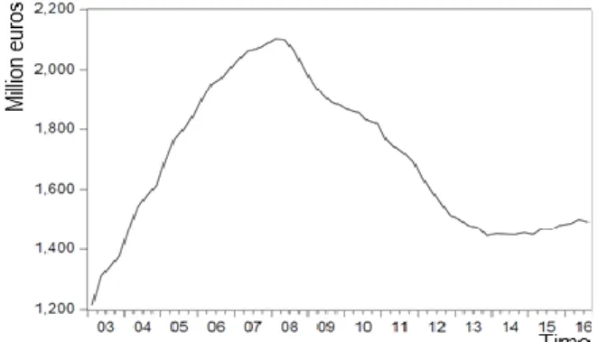
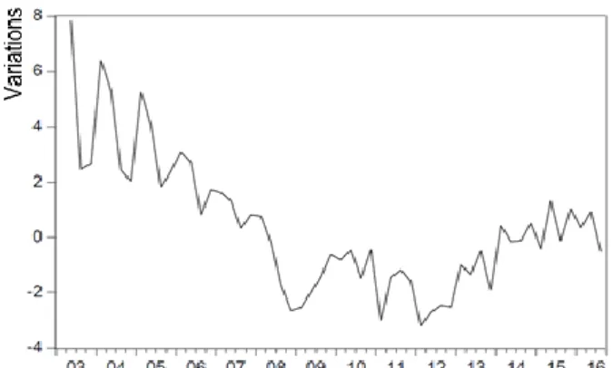
(14) 3.- Time series.. As explained above, the purpose of this study is to explain the evolution of real estate prices based on interest rates, mortgage concessions, foreign direct investment, per capita economic evolution and tourism. For this purpose, representative variables include the price per square meter of houses more than 5 years old, the mortgage interest rates over three years old, the monetary amount granted through mortgages divided by GDP per capita, the net income derived from international tourism and the net direct international investment position. Described the theoretical effects of the conditioning factors to be used, the price per square meter of houses more than 5 years old has been proposed as a study variable. This nuance is expected to provide a factor which contains homes with similar production costs. It is expected that innovations in construction materials produce lower production costs. The specific inclusion of this time series has been decided with the purpose of homogenizing the sample in this matter.. Figure 1: Evolution of price per square meter of houses more than 5 years old in Spain.. In Figure 1 it is observed the graphical representation of the chosen time series from 2003 to 2016. It is worth mentioning that the previous evolution is defined by a relatively stable trajectory until the beginning of the century. From this moment increases begin to accelerate to peak in the first quarter of 2008. The average price per square meter rose from 902€ in 2001 to 2102.1€ in 2008, representing an increase of 122.05%. Then there is a fall of 21.27% between 2008 and 2012. The latter variation positioned the price level at a more adequate level, confirming the bubble presence that burst in 2008 and ended up constituting the beginning of the financial and credit crisis. Finally, it should be mentioned that the series is expressed in euros, so a process to convert the series into 14.

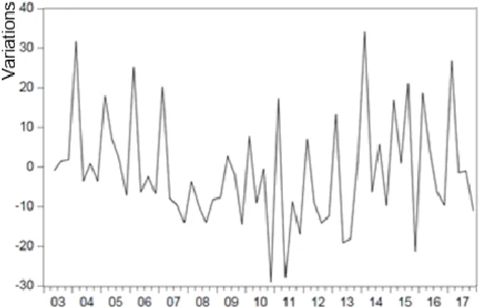
(15) variations is carried out to obtain percentage interpretations of the influences in the econometric model. Figure 2, shown below, offers the graphical representation of the converted variable used for the statistical model.. Figure 2: Evolution of the variations in the prices per square meter of houses more than 5 years old in Spain.. For statistical development, it has been decided to reflect the Euribor effects on prices through the use of average interest rates for mortgages over three years. The choice of this time series derived from private banking is motivated by the search for a variable that determines the final interests faced by the potential real estate consumer. The main reason for including bank margins within Euribor is justified in order to avoid a variables excess which could limit or reduce the explanatory capacities of the proposed econometric model. In relation to this argument, it should be mentioned that the sample available for the variables used is not very large. As mentioned previously, if this were not the case, a greater number of variables could be included or even a greater breakdown could be used.. 15.

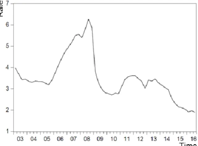
(16) Figure 3: Evolution of mortgage interest rates over three years for Spain.. Figure 3 shows the evolution of the series between 2003 and 2016. It is observed a stable trajectory, with interest rates between 3 and 4% until 2006. From this point on, the series begins to grow, reaching a maximum of 6.27% in the third quarter of 2008. From this peak, in less than two years, rates were drastically reduced to levels below those of the beginning of the millennium, showing decreases of more than three percentage points. In 2010, rates rise by around 3% and start to fall from 2014 to below 2% in 2016. Comparing with the previous series, a certain relationship can be seen, since, although with a certain lag, interest rates seem to negatively condition prices as predicted in the theoretical analysis. The variable has also been transformed into variations in order to obtain a more stable series. Figure 4 represents the transformed variable.. Figure 4: Evolution of variations in mortgage interest rates over three years for Spain... 16.

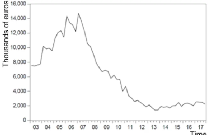
(17) In order to avoid the excess of variables and to obtain a model more in line with the size of the sample, it has been decided to incorporate as a temporary series the monetary amount granted through mortgages for the acquisition of all real estate types that is divided by the GDP per capita. This division produces a series that reflects the amount of credit granted by each monetary unit of GDP per capita. In other words, using this variable it is observed the monetary level granted through mortgages according to the national economic context in per capita terms. Below is Figure 5 containing the variable representation.. Figure 5: Evolution of the monetary amount granted through mortgages divided by GDP per capita for Spain.. Figure 5 shows a clear positive trend since the beginning of the century culminating in 2007, recording an increase of 95.23 % in only 4 years. From this turning point begins a serious fall in mortgage concessions that would end up reducing the figure by -90.41% between the peak credit moment and the third quarter of 2013, date from which it is observed a slow but stable recovery. As the theory had predicted, comparing the series trajectory with housing prices, it is observed a similar evolution, which indicates a positive relation, however, just as the previous series acts on our study variable with a certain lag. In order to obtain a series that offers better interpretations for the model it has been chosen to transform the series to variations. The definitive variable is reflected in Figure 6.. 17.

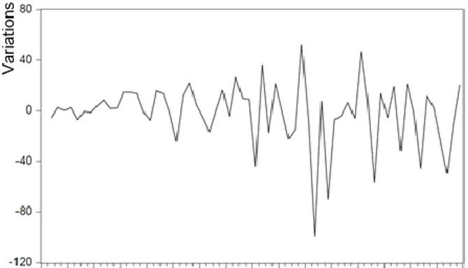
(18) Figure 6: Evolution of the variations in the monetary amount granted through mortgages divided by GDP per capita for Spain.. In order to include the foreign investment effects on real estate prices in the statistical model, the net international direct investment position has been included as variable. The series reflects net monetary amount imported or exported as direct investment. On the basis of the above theory, it is expected that prices rise in the face of the excessive investment arrival. In the face of high negative figures there could be indications of an over-investment in the country that could be inflating house prices. Rapid alterations in the variable are also expected to induce instabilities in the real estate market, which could attract or drive away new speculators to the market. Next, Figure 7 includes the graphical representation of the series.. Figure 7: Evolution of the net international investment position for Spain.. The time series shows high negative figures as a starting point. The investment position began to improve in 2005, with an investment withdrawal of more than 45% in less than 18.

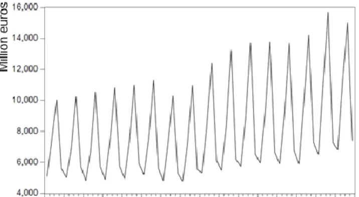
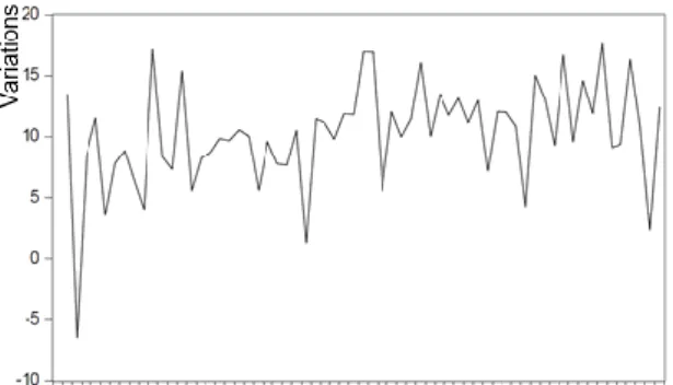
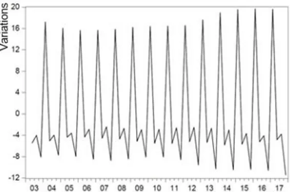
(19) two years. Between 2007 and 2012 a positive and stable reduction continues to be observed, which improved the position to a net investment import of 18444 million euros. From this date onwards, the series worsened again and for the next six years it was positioned in similar figures to those of 2006. Comparing the series trajectory with the evolution of real estate prices, there is a delayed relationship that reflects increases in prices in the face of high foreign investment inflows, on the contrary, the exit moments of this type of capitals induce decreases. For the definitive use of the series in the statistical model and in order to obtain better interpretations the series has been converted to variations. Figure 8 shows the graphical representation of the modified variable.. Figure 8: Evolution of the variations in the net international investment position for Spain.. In order to explain the above-mentioned tourism influences on the real estate prices level, it has been decided to use the net income from tourism as a time series. This variable reflects the income derived from the tourism reception, corrected by the expenses associated with the departure of national tourists. The data, collected from the Spanish balance of payments, have been represented in Figure 9. The representation offers a clear seasonality presence that is dealt later. Independently of the seasonal component, a slight but stable growth is observed until 2009, where there is a slight fall that is accompanied by a rapid recovery which ends up increasing the maximum and minimum figures by nearly 30% in 8 years. On the face of it, the series trajectory does not justify much of the price developments, however, it seems to contain some positive relationship that helped the bubble formation and reduced part of the subsequent depreciation. As with the previous variables, the series has been converted to variations to make it easier to use. The converted series is represented in Figure 10.. 19.

(20) Figure 9: Evolution of net income from international tourism for Spain.. Figure 10: Evolution of variations in net income from international tourism for Spain.. 20.

(21) 4.- Econometric model.. This document uses an autoregressive vectors model to define and reconcile the simultaneous interactions of the variables group with the exposed theoretical framework. A VAR is a model formed by a system of simultaneous equations in an unrestricted reduced form. The reduced form implies that the contemporary values of the model variables do not appear as explanatory variables in any equation, being constituted by a lags block of each one of the model series. On the other hand, the unrestricted form implies that the same explanatory variables group appears in each of them. Subsequently, in order to compare the impulse-response functions of the VAR model obtained, a transformed model is made, which includes order restrictions on the relationships between variables. This variant is defined as a structural VAR model and requires specifying the order of the series from lowest to highest exogeneity.. 4.1.- Necessary modifications.. Returning to the procedure, once the graphics representations of the used series have been visually analyzed, the first step to begin to develop the previously described models is to carry out different tests to confirm or detect the series anomalies that require correction. Seasonality settings are a potential modification. In order to statistically contrast the presence of this alteration in our set of variables, tests have been carried out using the X-11 seasonal adjustment methodology in its additive version. This module, contained in Eviews, executes several tests for the same purpose. Of the different results that the software offers us, those referring to the test for the presence of seasonality are valued, assuming stability. Beginning with the analysis of the results reported, included in Tables 4, 5, 6, 7 and 8 of the appendices, it is found the presence of seasonality in the series associated with tourism and in mortgage concessions over GDP per capita with a confidence level of 99%. Due to this, the seasonally adjusted series, represented in Figures 11 and 12 simultaneously, are used. The seasonal components of the decompositions carried out are also represented graphically. The latter (Figures 13 and 14) indicate the seasonal magnitude of both variables, with variations between 40 and 50% depending on the season for the tourist series and variations between 8 and 20% for the variable that contemplate the concessions.. 21.

(22) Figure 11: Evolution of seasonally adjusted variations in net income from international tourism in Spain.. Figure 12: Evolution of seasonally adjusted variations in the monetary amount granted through mortgages divided by GDP per capita for Spain.. Figure 13: Seasonal component of variations in net income from international tourism for Spain.. 22.

(23) Figure 14: Seasonal component of variations in the monetary amount granted through mortgages divided by GDP per capita for Spain.. 4.2.- Time series statistical analysis.. Once the necessary corrections and transformations have been made on the times series, the definitive variables statics, defined in Table 1, are analyzed. Among the descriptive statistics offered by Eviews, it is highlight the coefficient of skewness and kurtosis and the Jarque-Bera test. The latter compares the relationship between the kurtosis and skewness coefficients of the equation errors with those of a normal distribution, if these relationships are sufficiently different the null hypothesis of normal waste would be rejected. Based on the data received from the software and reflected in Table 1, it could be said that there is normality in all series except for loans granted through mortgages on GDP per capita.. V_MORT_IT. V_NET_TOUR_SA. V_NET_FOR_INV. V_CRED_GDP_PC_SA. V_PRICE. Mean. -1.01940. 9.95081. -1.12163. -1.12786. 0.41073. Median. -1.52073. 10.02108. 0.96923. -0.05356. -0.10974. Maximum. 12.96725. 17.11699. 51.78291. 24.63083. 7.92038. Minimum. -35.13835. -6.56313. -99.61663. -23.88803. -3.20960. Std.Dev.. 7.85037. 4.21484. 25.13372. 9.76662. 2.40712. Skewness. -1.30342. -1.04600. -1.43655. -0.17920. 0.93735. Kurtosis. 7.98782. 5.99985. 7.12321. 3.25119. 3.82853. Jarque-Bera. 71.26630. 30.09494. 56.82511. 0.43099. 9.45212. Probability. 0.00000. 0.00000. 0.00000. 0.80614. 0.00886. Sum Sq. Dev.. 3266.29900. 941.53790. 33480.31000. 5055.50400. 307.09420. Observations. 54. 54. 54. 54. 54. Table 1: Individual statistics of the series group used... 23.

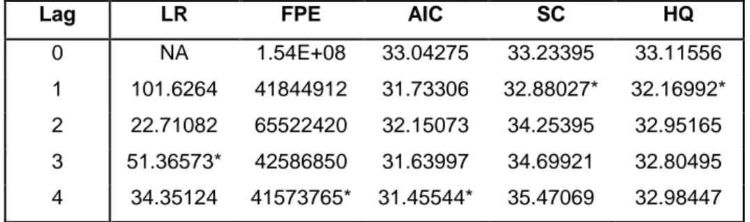
(24) Table 2 shows the correlation matrix of the series, which gives an overview of the relationships between the definitive variables in a simple and contemporary way. Focusing on the relations of the series on price, a greater influence of mortgage concessions on GDP per capita is observed, followed by tourism. With lower correlation it is found the net investment position and bank interest rates. Another conclusion offered by the matrix derives from the correlation shown by practically all the variables, which justifies the use of simultaneous models such as those to be carried out. Another way of carrying out this type of preliminary analysis could be by means of Granger causality tests. These tests verify whether a variable serves to predict the evolution of another, while indicating whether the relationship is unidirectional or bidirectional.. V_MORT_IT. V_NET_TOUR_SA. V_NET_FOR_INV. V_CRED_GDP_PC_SA. V_PRICE. V_MORT_IT. 1.00000. 0.20484. 0.07925. 0.04285. 0.12310. V_NET_TOUR_SA. 0.20484. 1.00000. -0.09474. -0.12349. -0.22508. V_NET_FOR_INV. 0.07925. -0.09474. 1.00000. -0.14537. 0.12879. V_CRED_GDP_PC_SA. 0.04285. -0.12349. -0.14537. 1.00000. 0.42351. V_PRICE. 0.12310. -0.22508. 0.12879. 0.42351. 1.00000. Table 2: Correlation matrix of the series used... 4.3.- Lag-order selection.. Once the modified time series are defined and ready for use, the order of the model is defined, that is, the lag until which the incorporated information is statistically significant. Choosing a high number of lags for a relatively small sample could cause degrees of freedom to run out quickly and result in large standard errors in estimates. This fact would increase the confidence intervals of the model coefficients, so it has been decided to estimate the mentioned criteria on a maximum of 4 lags. In order to carry out this step, a VAR model is created with the predefined criteria offered by Eviews, so that once inside, a test is executed to obtain the indicates shown in Table 3, how many lags it is recommended to use in estimating the model, offering the values of information criteria such as Akaike, Schwartz, Hannan-Quinn or the Likelihood ratio, among others, with the suggestions of each one being highlighted with a "*".. 24.

(25) Lag. LR. FPE. AIC. SC. HQ. 0. NA. 1.54E+08. 33.04275. 33.23395. 33.11556. 1. 101.6264. 41844912. 31.73306. 32.88027*. 32.16992*. 2. 22.71082. 65522420. 32.15073. 34.25395. 32.95165. 3. 51.36573*. 42586850. 31.63997. 34.69921. 32.80495. 4. 34.35124. 41573765*. 31.45544*. 35.47069. 32.98447. Table 3: VAR lag order selection criteria.. It can be seen that the criteria offer different conclusions. In view of the disparity, the order to be used is determined by the parsimony principle, i.e. by the least possible order. This should be done taking into account that there is no correlation between the residues of the different equations. Tables 9 and 10 in the appendices show the results of the residual serial correlation test. From these it is concluded, with a confidence level of more than 95%, that the minimum order for which no correlation is found is 4 lags.. 4.4.- Model formulation.. With the known lags and the transformed variables, it is possible to formulate the VAR model. It is defined by the following system of five equations, where V_Mort_IT represents the evolution of variations in mortgage interest rates over 3 years, V_Net_For_Inv represents the evolution of variations in net international direct investment position, V_Net_Tour_sa represents the evolution of seasonally adjusted variations in net income from international tourism, V_Cred_Gran_GDP_pc_sa represents the evolution of seasonally adjusted variations in the monetary amount granted through mortgages divided by GDP per capita, V_Price represents the evolution of variations in the price per square meter of houses more than 5 years old. β represent intercepts and parameters which show the effects of the different series lags on the contemporary variables explained. Finally, there are the error terms (𝑢) for each equation.. 𝑉_𝑀𝑜𝑟𝑡_𝐼𝑇𝑡 = 𝛽10 +. 𝛽101 𝑉_𝑀𝑜𝑟𝑡_𝐼𝑇𝑡−1 + 𝛽102 𝑉_𝑁𝑒𝑡_𝑇𝑜𝑢𝑟_𝑠𝑎𝑡−1 + 𝛽103 𝑉_𝑁𝑒𝑡_𝐹𝑜𝑟_𝐼𝑛𝑣𝑡−1 +. 𝛽104 𝑉_𝐶𝑟𝑒𝑑_𝐺𝑟𝑎𝑛_𝐺𝐷𝑃_𝑝𝑐_𝑠𝑎𝑡−1. 𝛽105 𝑉_𝑃𝑟𝑖𝑐𝑒𝑡−1. +. +. 𝛽106 𝑉_𝑀𝑜𝑟𝑡_𝐼𝑇𝑡−2. +. 𝛽107 𝑉_𝑁𝑒𝑡_𝑇𝑜𝑢𝑟_𝑠𝑎𝑡−2 + 𝛽108 𝑉_𝑁𝑒𝑡_𝐹𝑜𝑟_𝐼𝑛𝑣𝑡−2 + 𝛽109 𝑉_𝐶𝑟𝑒𝑑_𝐺𝑟𝑎𝑛_𝐺𝐷𝑃_𝑝𝑐_𝑠𝑎𝑡−2 + 𝛽110 𝑉_𝑃𝑟𝑖𝑐𝑒𝑡−2 + 𝛽111 𝑉_𝑀𝑜𝑟𝑡_𝐼𝑇𝑡−3 + 𝛽112 𝑉_𝑁𝑒𝑡_𝑇𝑜𝑢𝑟_𝑠𝑎𝑡−3 + 𝛽113 𝑉_𝑁𝑒𝑡_𝐹𝑜𝑟_𝐼𝑛𝑣𝑡−3 +. 25.

(26) 𝛽114 𝑉_𝐶𝑟𝑒𝑑_𝐺𝑟𝑎𝑛_𝐺𝐷𝑃_𝑝𝑐_𝑠𝑎𝑡−3. 𝛽115 𝑉_𝑃𝑟𝑖𝑐𝑒𝑡−3. +. 𝛽116 𝑉_𝑀𝑜𝑟𝑡_𝐼𝑇𝑡−4. +. +. 𝛽117 𝑉_𝑁𝑒𝑡_𝑇𝑜𝑢𝑟_𝑠𝑎𝑡−4 + 𝛽118 𝑉_𝑁𝑒𝑡_𝐹𝑜𝑟_𝐼𝑛𝑣𝑡−4 + 𝛽119 𝑉_𝐶𝑟𝑒𝑑_𝐺𝑟𝑎𝑛_𝐺𝐷𝑃_𝑝𝑐_𝑠𝑎𝑡−4 + 𝛽120 𝑉_𝑃𝑟𝑖𝑐𝑒𝑡−4 + 𝑢1𝑡. 𝑉_𝑁𝑒𝑡_𝑇𝑜𝑢𝑟_𝑠𝑎𝑡 = 𝛽20 + 𝛽201 𝑉_𝑀𝑜𝑟𝑡_𝐼𝑇𝑡−1 + 𝛽202 𝑉_𝑁𝑒𝑡_𝑇𝑜𝑢𝑟_𝑠𝑎𝑡−1 + 𝛽203 𝑉_𝑁𝑒𝑡_𝐹𝑜𝑟_𝐼𝑛𝑣𝑡−1 + 𝛽204 𝑉_𝐶𝑟𝑒𝑑_𝐺𝑟𝑎𝑛_𝐺𝐷𝑃_𝑝𝑐_𝑠𝑎𝑡−1. 𝛽205 𝑉_𝑃𝑟𝑖𝑐𝑒𝑡−1. +. 𝛽206 𝑉_𝑀𝑜𝑟𝑡_𝐼𝑇𝑡−2. +. +. 𝛽207 𝑉_𝑁𝑒𝑡_𝑇𝑜𝑢𝑟_𝑠𝑎𝑡−2 + 𝛽208 𝑉_𝑁𝑒𝑡_𝐹𝑜𝑟_𝐼𝑛𝑣𝑡−2 + 𝛽209 𝑉_𝐶𝑟𝑒𝑑_𝐺𝑟𝑎𝑛_𝐺𝐷𝑃_𝑝𝑐_𝑠𝑎𝑡−2 + 𝛽210 𝑉_𝑃𝑟𝑖𝑐𝑒𝑡−2 + 𝛽211 𝑉_𝑀𝑜𝑟𝑡_𝐼𝑇𝑡−3 + 𝛽212 𝑉_𝑁𝑒𝑡_𝑇𝑜𝑢𝑟_𝑠𝑎𝑡−3 + 𝛽213 𝑉_𝑁𝑒𝑡_𝐹𝑜𝑟_𝐼𝑛𝑣𝑡−3 + 𝛽214 𝑉_𝐶𝑟𝑒𝑑_𝐺𝑟𝑎𝑛_𝐺𝐷𝑃_𝑝𝑐_𝑠𝑎𝑡−3. 𝛽215 𝑉_𝑃𝑟𝑖𝑐𝑒𝑡−3. +. 𝛽216 𝑉_𝑀𝑜𝑟𝑡_𝐼𝑇𝑡−4. +. +. 𝛽217 𝑉_𝑁𝑒𝑡_𝑇𝑜𝑢𝑟_𝑠𝑎𝑡−4 + 𝛽218 𝑉_𝑁𝑒𝑡_𝐹𝑜𝑟_𝐼𝑛𝑣𝑡−4 + 𝛽219 𝑉_𝐶𝑟𝑒𝑑_𝐺𝑟𝑎𝑛_𝐺𝐷𝑃_𝑝𝑐_𝑠𝑎𝑡−4 + 𝛽220 𝑉_𝑃𝑟𝑖𝑐𝑒𝑡−4 + 𝑢2𝑡. 𝑉_𝑁𝑒𝑡_𝐹𝑜𝑟_𝐼𝑛𝑣𝑡 = 𝛽30 + 𝛽301 𝑉_𝑀𝑜𝑟𝑡_𝐼𝑇𝑡−1 + 𝛽302 𝑉_𝑁𝑒𝑡_𝑇𝑜𝑢𝑟_𝑠𝑎𝑡−1 + 𝛽303 𝑉_𝑁𝑒𝑡_𝐹𝑜𝑟_𝐼𝑛𝑣𝑡−1 + 𝛽304 𝑉_𝐶𝑟𝑒𝑑_𝐺𝑟𝑎𝑛_𝐺𝐷𝑃_𝑝𝑐_𝑠𝑎𝑡−1. 𝛽305 𝑉_𝑃𝑟𝑖𝑐𝑒𝑡−1. +. 𝛽306 𝑉_𝑀𝑜𝑟𝑡_𝐼𝑇𝑡−2. +. +. 𝛽307 𝑉_𝑁𝑒𝑡_𝑇𝑜𝑢𝑟_𝑠𝑎𝑡−2 + 𝛽308 𝑉_𝑁𝑒𝑡_𝐹𝑜𝑟_𝐼𝑛𝑣𝑡−2 + 𝛽309 𝑉_𝐶𝑟𝑒𝑑_𝐺𝑟𝑎𝑛_𝐺𝐷𝑃_𝑝𝑐_𝑠𝑎𝑡−2 + 𝛽310 𝑉_𝑃𝑟𝑖𝑐𝑒𝑡−2 + 𝛽311 𝑉_𝑀𝑜𝑟𝑡_𝐼𝑇𝑡−3 + 𝛽312 𝑉_𝑁𝑒𝑡_𝑇𝑜𝑢𝑟_𝑠𝑎𝑡−3 + 𝛽313 𝑉_𝑁𝑒𝑡_𝐹𝑜𝑟_𝐼𝑛𝑣𝑡−3 + 𝛽314 𝑉_𝐶𝑟𝑒𝑑_𝐺𝑟𝑎𝑛_𝐺𝐷𝑃_𝑝𝑐_𝑠𝑎𝑡−3. 𝛽315 𝑉_𝑃𝑟𝑖𝑐𝑒𝑡−3. +. 𝛽316 𝑉_𝑀𝑜𝑟𝑡_𝐼𝑇𝑡−4. +. +. 𝛽317 𝑉_𝑁𝑒𝑡_𝑇𝑜𝑢𝑟_𝑠𝑎𝑡−4 + 𝛽318 𝑉_𝑁𝑒𝑡_𝐹𝑜𝑟_𝐼𝑛𝑣𝑡−4 + 𝛽319 𝑉_𝐶𝑟𝑒𝑑_𝐺𝑟𝑎𝑛_𝐺𝐷𝑃_𝑝𝑐_𝑠𝑎𝑡−4 + 𝛽320 𝑉_𝑃𝑟𝑖𝑐𝑒𝑡−4 + 𝑢3𝑡. 𝑉_𝐶𝑟𝑒𝑑_𝐺𝑟𝑎𝑛_𝐺𝐷𝑃_𝑝𝑐_𝑠𝑎𝑡. 𝛽40. =. 𝛽403 𝑉_𝑁𝑒𝑡_𝐹𝑜𝑟_𝐼𝑛𝑣𝑡−1 𝛽406 𝑉_𝑀𝑜𝑟𝑡_𝐼𝑇𝑡−2. + +. 𝛽401 𝑉_𝑀𝑜𝑟𝑡_𝐼𝑇𝑡−1. +. +. 𝛽402 𝑉_𝑁𝑒𝑡_𝑇𝑜𝑢𝑟_𝑠𝑎𝑡−1. +. 𝛽405 𝑉_𝑃𝑟𝑖𝑐𝑒𝑡−1. +. 𝛽404 𝑉_𝐶𝑟𝑒𝑑_𝐺𝑟𝑎𝑛_𝐺𝐷𝑃_𝑝𝑐_𝑠𝑎𝑡−1 𝛽407 𝑉_𝑁𝑒𝑡_𝑇𝑜𝑢𝑟_𝑠𝑎𝑡−2. 𝛽409 𝑉_𝐶𝑟𝑒𝑑_𝐺𝑟𝑎𝑛_𝐺𝐷𝑃_𝑝𝑐_𝑠𝑎𝑡−2. +. 𝛽410 𝑉_𝑃𝑟𝑖𝑐𝑒𝑡−2. +. +. 𝛽408 𝑉_𝑁𝑒𝑡_𝐹𝑜𝑟_𝐼𝑛𝑣𝑡−2 +. 𝛽411 𝑉_𝑀𝑜𝑟𝑡_𝐼𝑇𝑡−3. + +. 𝛽412 𝑉_𝑁𝑒𝑡_𝑇𝑜𝑢𝑟_𝑠𝑎𝑡−3 + 𝛽413 𝑉_𝑁𝑒𝑡_𝐹𝑜𝑟_𝐼𝑛𝑣𝑡−3 + 𝛽414 𝑉_𝐶𝑟𝑒𝑑_𝐺𝑟𝑎𝑛_𝐺𝐷𝑃_𝑝𝑐_𝑠𝑎𝑡−3 + 𝛽415 𝑉_𝑃𝑟𝑖𝑐𝑒𝑡−3 + 𝛽416 𝑉_𝑀𝑜𝑟𝑡_𝐼𝑇𝑡−4 + 𝛽417 𝑉_𝑁𝑒𝑡_𝑇𝑜𝑢𝑟_𝑠𝑎𝑡−4 + 𝛽418 𝑉_𝑁𝑒𝑡_𝐹𝑜𝑟_𝐼𝑛𝑣𝑡−4 + 𝛽419 𝑉_𝐶𝑟𝑒𝑑_𝐺𝑟𝑎𝑛_𝐺𝐷𝑃_𝑝𝑐_𝑠𝑎𝑡−4 + 𝛽420 𝑉_𝑃𝑟𝑖𝑐𝑒𝑡−4 + 𝑢1𝑡. 𝑉_𝑃𝑟𝑖𝑐𝑒𝑡 = 𝛽50 +. 𝛽501 𝑉_𝑀𝑜𝑟𝑡_𝐼𝑇𝑡−1 + 𝛽502 𝑉_𝑁𝑒𝑡_𝑇𝑜𝑢𝑟_𝑠𝑎𝑡−1 + 𝛽503 𝑉_𝑁𝑒𝑡_𝐹𝑜𝑟_𝐼𝑛𝑣𝑡−1 +. 𝛽504 𝑉_𝐶𝑟𝑒𝑑_𝐺𝑟𝑎𝑛_𝐺𝐷𝑃_𝑝𝑐_𝑠𝑎𝑡−1. 𝛽505 𝑉_𝑃𝑟𝑖𝑐𝑒𝑡−1. +. +. 𝛽506 𝑉_𝑀𝑜𝑟𝑡_𝐼𝑇𝑡−2. +. 𝛽507 𝑉_𝑁𝑒𝑡_𝑇𝑜𝑢𝑟_𝑠𝑎𝑡−2 + 𝛽508 𝑉_𝑁𝑒𝑡_𝐹𝑜𝑟_𝐼𝑛𝑣𝑡−2 + 𝛽509 𝑉_𝐶𝑟𝑒𝑑_𝐺𝑟𝑎𝑛_𝐺𝐷𝑃_𝑝𝑐_𝑠𝑎𝑡−2 + 𝛽510 𝑉_𝑃𝑟𝑖𝑐𝑒𝑡−2 + 𝛽511 𝑉_𝑀𝑜𝑟𝑡_𝐼𝑇𝑡−3 + 𝛽512 𝑉_𝑁𝑒𝑡_𝑇𝑜𝑢𝑟_𝑠𝑎𝑡−3 + 𝛽513 𝑉_𝑁𝑒𝑡_𝐹𝑜𝑟_𝐼𝑛𝑣𝑡−3 + 𝛽514 𝑉_𝐶𝑟𝑒𝑑_𝐺𝑟𝑎𝑛_𝐺𝐷𝑃_𝑝𝑐_𝑠𝑎𝑡−3. 𝛽515 𝑉_𝑃𝑟𝑖𝑐𝑒𝑡−3. +. +. 𝛽516 𝑉_𝑀𝑜𝑟𝑡_𝐼𝑇𝑡−4. +. 𝛽517 𝑉_𝑁𝑒𝑡_𝑇𝑜𝑢𝑟_𝑠𝑎𝑡−4 + 𝛽518 𝑉_𝑁𝑒𝑡_𝐹𝑜𝑟_𝐼𝑛𝑣𝑡−4 + 𝛽519 𝑉_𝐶𝑟𝑒𝑑_𝐺𝑟𝑎𝑛_𝐺𝐷𝑃_𝑝𝑐_𝑠𝑎𝑡−4 + 𝛽520 𝑉_𝑃𝑟𝑖𝑐𝑒𝑡−4 + 𝑢5𝑡. 26.

(27) When the equations system is estimated, the estimators and some statistics of the proposed model are specified. The results are included in Table 11 of the appendices because of their length. It is composed by three blocks. The first, positioned at the top, collects the general characteristics of the estimate made, such as the time series used, the estimation method used, the sample period (2003Q2:2015Q3) and the actual sample size. Second, there is individual information about each of the variables, including the name, the estimated coefficients value, the standard deviation of those coefficients, and the statistic t values. Finally, the third block includes a series of joint statistics, where it could be found the determination coefficient and its corrected equivalent, the estimated value of the error standard deviation, the quadratic sum of waste, the final value of the maximum likelihood logarithm or the values for the lag selection criteria among others. It should be mentioned that the results offered by Eviews could be used for hypothesis testing and therefore for predictions, however, the seasonality adjustments should be included if you want to focus the model for that purpose. However, it has not been executed in this document due to the estimates purposed of autoregressive models are limited to examining the relationships between the variables. Differentiation processes that would eliminate the trend could suppress relevant short-term information and only allow the model to identify long-term relationships.. 4.5.- Impulse Response functions.. In order to obtain the desired estimates, impulse-response functions are used, by means of this it is obtained relations that represent the effects on one variable when faced with a shock in another. More specifically, these are orthogonal shocks, which by definition do not incorporate correlation with the rest of contemporary shocks. It should be noted that obtaining VAR and SVAR models for this case begin to differ in the orthogonal decomposition variant to use. For the VAR model a generalized decomposition is used and for the SVAR models an orderly decomposition of Cholensky adjusted by freedom degrees is used. The representations in Figure 15 show the impulse response functions referring to the VAR model, where the simultaneity effects are assumed and no order is indicated on the impulses. In order to carry them out, the simulation period following the shock to be analyzed is specified, including five years for this purpose, and only the functions that explain the price trajectory are included. The other representations have been included in Figure 19 of the appendices. Prior to the valuation it should be mentioned that the 27.

(28) shocks of the impulse response functions are induced with the standard deviation magnitude, which is the usual alteration suffered by the factor. As might be expected based on the above, analyzing Figure 15, in the face of a shock on the interest rates variation, a negative conditioning on the price level is observed. The influence begins to take effect from the second quarter, to have its greatest shock between the third and eighth, then the negative variations decrease until they disappear. It is worth mentioning that the reduction is in variations terms, so the series actually be negatively affected. The fact can be observed with the generalized response impulse functions whose responses are cumulative. The functions included in Figure 20 of the appendices show how this shock can reduce the price by more than 2% in three years. Observing the conditioning produced in the prices by the net income of international tourism, a negative but unstable influence is observed, with values close to zero. The representation shows greater influence during the first three years. The graphs with cumulative responses (Figure 20 of the appendices) indicate a brief conditioning, close to the 1.6% reached in ten quarters. Contrary to previous expectations, increases in net income associated with tourism, far from raising real estate prices, reduce them. On the other hand, net foreign investment shows a high influence on the main study variable. In the event of a shock, there is a noticeable reduction in prices. The expected falls are increasing until the second year, when begin to reduce until disappear in the fifth. From the perspective of the accumulated results, in the face of the shock, it is expected that prices fall by close to 5%. The negative relationship is consistent with the above theory. The impulse response functions also show how the shock on the amount of credit granted divided by GDP per capita produces a positive conditioning on house prices. The impact increases during the first year and then begins to decrease to offer variations close to zero between the fourth and fifth year. In relation to the cumulative response contained in Figure 20 of the appendices, a total increase of about 2.5% can be observed. The results are consistent with the data presented in the previous theory. Finally, it is price variations trajectory in the face of price shock. The relationship indicates a clear positive but volatile autocorrelation which approaches zero from the third year onwards, indicating that part of the evolution is explained by past behavior of no more than three years. This assertion is due to price increases produce on the expectations of regular investors and consumers.. 28.

(29) Figure 15: Response impulse functions with generalized orthogonal shocks.. In order to obtain more precise specifications, it is proposed to obtain the impulse response functions by means of Cholensky orthogonal decomposition. Through this process, the VAR results are obtained structurally. This variant allows to induce order on the variables from greater to lesser degree of exogeneity with respect to the housing prices, allowing a specification with which it is expected to obtain more significant results. Cholensky decomposition completely incorporates the alteration produced by the first factor over the others. The second and subsequent shocks only incorporate influences that have not been included by the previous ones. With respect to Cholensky procedure, it should be noted that shocks have the same interpretation as obtained through. 29.

(30) generalized impulses, in such a way that the functions represent the price variations produced by impulses of a standard deviation in the determining factors. Based on the above, two different interaction orders are proposed for the development of this section. Depending on the theoretical framework, the interest rate on the left is respected because it is the most independent variable of the group and is followed by international tourism that not move either. At an intermediate point it is found the net direct investment and the monetary amount granted through mortgage divided by GDP per capita. Finally, prices always go to the right as the most dependent factor of the previous ones. From the two possible combinations, based on changing the order of interaction between the net direct investment and credit amounts granted, the two proposed models emerge. The Figure 16 functions represent the first variant, where net foreign investment shock anticipates credit granted over GDP per capita. As has been done with the generalized imposed response functions, only the graphs that justify the effects on real estate prices are included, the others are included in Figure 21 of the appendices. Analyzing the representations, it is observed conditions practically identical to those obtained by means of generalized impulses. However, the new specification does slightly reduce the effects of tourism on price, bringing them even closer to 0. Analyzing the cumulative responses of the relationship, it is observed a fall in influence close to 0.9% in the face of the shock. Finally, it is worth mentioning the presence of a slightly more abrupt conditioning of net foreign direct investment on the price level.. 30.

(31) Figure 16: Response impulse functions with orthogonal Cholensky shocks for the first order proposed.. Taking into account the impulse response functions of the second proposal (Figure 17), where the credit variation over GDP per capita precedes net foreign investment, practically identical results are obtained to those obtained through the previous structure. The functions show the same discrepancies with the functions obtained by generalized pulses. In spite of the slight differences present in the three variants, the results obtained are practically the same. Comparing the cumulative response functions (Figures 20, 22 and 23 in the appendices), the total influences differ by a maximum of 0.9%, with shocks in tourism and credit granted divided by GDP per capita. There are no differences for influences on mortgage interest rates. 31.

(32) Figure 17: Response impulse functions with orthogonal Cholensky shocks for the second order proposed.. The similarity of the results obtained through the three methods shows the simultaneity influence of the effects and therefore implies the irrelevance of inducing order for the orthogonal decomposition, making possible to make conclusions based on the VAR model results and not incurring in specification problems. Finally, it should be noted that the functions obtained do not show explosive dynamic relationships, indicating that past effects do not have a greater impact than present ones. This fact confirms that the statistical models used make sense and are useful for the purposes of the document. 32.

(33) 4.6.- Variance decomposition.. Figure 18: Variance decomposition of the housing price prediction errors.. As an additional study to the previous functions, the error variance is decomposed. This procedure shows the percentage of error induced on the prices evolution by the shocks in the explanatory factors in the different moments of the simulation. In other words, it separates the variance from the forecast error for each factor. Figure 18 shows the variance decomposition representation of the real estate price prediction errors. The other graphs are included in Figure 24 of the appendices.. 33.

(34) With regard to decomposition, there is a greater variance induced by net foreign investment and by the same prices. The first factor shows a starting justification of 10% that increases over the first three years to 40% to be maintained until the end of the simulation. The second factor mentioned above shows an induction to price volatility of 60%, that is reduced in the first three years to close to 20%, which is a strong volatility induced by the autoregressive component during the first twelve quarters. The impulses on the net income derived from international tourism show a decreasing influence in the price behavior variance which starts from a 20% and is reduced by half in little more than two and a half years. With less influence are observed the interest rate shocks that justify about 15% of the error variance that begins to make effective after the first year, until then induced variance is around 5%. Finally, it should be mentioned that the shocks to the mortgage credit granted over GDP per capita justify a maximum of 12% of the confidence interval. Reaching the maximum values from the sixth quarter onwards.. 34.

(35) 5.- Conclusion. The previous theory indicates a clear negative relationship between mortgage interest rates and house prices, this proposal has been statistically confirmed in the econometric model variants. It is confirmed that mortgage lending has a positive relationship on real estate prices. The clear negative relationship between the net foreign investment position and the real estate prices level is also confirmed. This ratio weighs twice as much as the effects induced by consumer interest rates in the event of a shock to the corresponding standard deviations. With regard to the influence of net income from international tourism, a statistical relation very close to zero is observed. In addition to the wide confidence intervals one cannot conclude objective results on this relationship. Finally, there is a positive autocorrelation of the price factor that presents some volatility. This fact was to be expected due to the speculative component explained in advance. Ordering the effects by relevance, greater cumulative influence has been obtained from net foreign investment, followed by interest rates, the mortgage credit granted on per capita GDP and its own autoregressive component. Finally, with a brief impact contrary to the theory presented in the document, is the influence of net income from tourism. It is necessary to comment that the confidence intervals of the impulse response functions, created at 95% confidence, are relatively wide, because of this, the predicted results may not be accurate enough. In addition to the above, it should be noted that much of the error variance induced in the price explanation is motivated by the impulses on net foreign investment and by its own autoregressive component. The recent entry of the Spanish economy into monetary union produces relatively short time series. This problem makes it impossible to enrich the explanation by including more variables or breaking down the existing ones. In view of an increase in the series sample size, the breakdown of mortgage interest rates over three years in Euribor and bank margins, including the GDP per capita separately and divide the credit granted by the housing stock could be useful. The model could also be improved with the inclusion of variables such as the average rental prices, unemployment, the banking sector profits, the average years of real estate possession, the social housing production, the reclassifications carried out or even some exchange rate referring to the euro against a currency basket which contemplates the most important economies in the world. Finally, it is worth mentioning the possibility of carrying out an extension by including a vector error correction model (VEC), which would offer a breakdown of the relations between the short and long term.. 35.

(36) This document verifies the broad relationship between available market liquidity and real estate prices. Particularly noteworthy is the net direct investment position. The results also indicate the importance of monitoring interest rates and mortgage concessions to prevent real estate bubbles. The Euribor, as an instrument of monetary control of the European Central Bank, follows logical paths that facilitate the Eurozone economic development. However, the problem of organizing a multitude of economies under the same policy can produce synchronization difficulties depending on the needs of each country, which can cause serious imbalances in some. Governments need to pay greater attention to excess liquidity in markets, implementing policies that prevent credit overexpansions and unstable foreign investment inflows. With the literature prior to the conduct of the study is observed as society, governments, institutions and analysts are more informed and therefore it is unlikely that the appropriate measures will not be taken if the economy begins to show excessive debt levels which could be feeding bubbles. In relation to international tourism, there is not statistical evidence that implies a high influence on the price level, so it could be suppressed and replaced by another variable which could improve the explanatory power. Prices are currently experiencing a slow and stable growth that is likely to continue. Speculation may have been the biggest conditioning factor in the formation of the real estate bubble. It is necessary to mention that this kind of investors can reach any market and are hardly detectable until the bubble formed explodes. Thus, once again, it is governments and institutions who must avoid overinvestments by developing financial regulations which limit this type of operation when necessary.. 36.

(37) 6.- Appendices.. Sum. Of. Dgrs. Of. Mean. Squares. Freedom. Square. F-Value. Between quarters. 114789.8981. 3. 38263.29938. 1063.016**. Residual. 2123.7069. 59. 35.99503. Total. 116913.6051. 62. Table 4: Seasonality test on evolution of variations in the net income derived from international tourism.. Dgrs. Of. Mean. Sum. Of Squares. Freedom. Square. F-Value. Between quarters. 6007.1909. 3. 2002.39697. 41.504**. Residual. 2653.5025. 55. 48.2455. Total. 8660.6934. 58. Table 5: Seasonality test on evolution of variations in the monetary amount granted through mortgages divided by GDP per capita for Spain.. Dgrs. Of. Mean. Sum. Of Squares. Freedom. Square. F-Value. Between quarters. 8.3450. 3. 2.78166. 4.784. Residual. 29.0732. 50. 0.58146. Total. 37.4181. 53. Table 6: Seasonality test on evolution of the variations in the prices per square meter of houses more than 5 years old in Spain.. Dgrs. Of. Mean. Sum. Of Squares. Freedom. Square. F-Value. Between quarters. 62.2060. 3. 20.73532. 1.309. Residual. 791.8554. 50. 15.83711. Total. 854.0613. 53. Table 7: Seasonality test on the evolution of variations in mortgage interest rates over three years for Spain.. 37.

(38) Dgrs. Of. Mean. Sum. Of Squares. Freedom. Square. F-Value. Between quarters. 1114.6030. 3. 371.53433. 0.814. Residual. 26945.8234. 59. 456.70887. Total. 28060.4263. 62. Table 8: Seasonality test on the evolution of variations in the net international investment position for Spain.. Table 9: VAR Residual Correlation LM Tests for 3 lags.. 38.

(39) Table 10: VAR Residual Correlation LM Tests for 4 lags.. 39.

(40) 40.

(41) Table 11: Vector autoregression estimates.. 41.

(42) Figure 19: Rest of impulse response functions with generalized orthogonal shocks.. 42.

(43) Figure 20: Response impulse functions with generalized orthogonal shocks and accumulated responses.. 43.

(44) Figure 21: Rest of impulse response functions with orthogonal Cholensky shocks for the first order proposed. 44.

(45) Figure 22: Response impulse functions with orthogonal Cholensky shocks and accumulated responses for the first proposed order. 45.

(46) Figure 23: Response impulse functions with orthogonal Cholensky shocks and accumulated responses for the second proposed order.. 46.

(47) Figure 24: Rest of error variance decomposition functions.. 47.

(48) 7.- References.. Carbó, S. and Rodríguez, F. (2008). ‘The relationship between mortgage markets and house prices: Does financial instability make the difference?’ University of Granada online. Downloaded from: https://www.ugr.es/~scarbo/Mortgage.pdf [Accessed 5 June 2019] Goodhart, C. and Hofmann, B. (2008). House Prices, Money, Credit and The Macroeconomy. Frankfurt: European Central Bank. Available at: https://www.ecb.europa.eu/pub/pdf/scpwps/ecbwp888.pdf?aae25e46c7906056e754b9 d641d0c10f [Accessed 5 June 2019]. Rogers, R., Wong, A. and Nelson, J. (2017) ‘Public perceptions of foreign and Chinese real estate investment: intercultural relations in Global Sydney’. Australian Geographer, 437- 455. Available at: https://www.researchgate.net/publication/316805127_Public_perceptions_of_foreign_a nd_Chinese_real_estate_investment_intercultural_relations_in_Global_Sydney [Accessed 5 June 2019]. 48.

(49) 8.- Bibliography.. Anundsen, A. and Jansen, E. (2013) ‘Self- reinforcing effects between housing prices and credit’. Journal of Housing Economics 22. Issue 3, 192-212. Available at: https://www.sciencedirect.com/science/article/pii/S1051137713000338 [Accessed 5 June 2019] Brooks, C. (2008) Introductory Econometrics for Finance. New York: Cambridge University Press. Available at: https://www.cambridge.org/es/academic/subjects/economics/finance/introductoryeconometrics-finance-4th-edition?format=PB&isbn=9781108422536 [Accessed 5 June 2019] Cesa-Bianchi, A., Cespedes, L. and Rebucci A. (2015) ‘Global Liquidity, House Prices, and the Macroeconomy: Evidence from Advanced and Emerging Economies’. International Monetary Fund online. Downloaded from: https://pdfs.semanticscholar.org/6f56/539b6cf66b2b0d149db368282c4d3a140d2f.pdf [5 June 2019] Eerola, E. and Määttänen, N. (2018) ‘Borrowing constraints and housing liquidity’. Review of Economic Dynamics 27, 184-204. Available at: https://www.sciencedirect.com/science/article/pii/S1094202517300601 [Accessed 5 June 2019] Van Dijik, D. and Francke, M. (2015) ‘Internet search behavior, liquidity and prices in the housing market’ DeNederlandscheBank 481, 1-34. Available at: https://www.dnb.nl/binaries/Working%20paper%20481_tcm46-325317.pdf [Accessed 5 June 2019] Vigdor, J. (2004) ‘Liquidity constraints and housing prices: Theory and evidence from the VA Mortgae’ National Bureau of Economic Research online. Downloaded from: https://www.nber.org/papers/w10611.pdf [5 June 2019]. 49.

(50) 9.- Database sources.. Evolution of mortgage interest rates over three years for Spain: http://www.ine.es/jaxi/Tabla.htm?path=/t38/p604/a2000/&file=0902001.px Evolution of net income from international tourism for Spain: https://www.bde.es/bde/es/areas/estadis/Otras_estadistic/Reservas_interna/ Evolution of price per square meter of houses more than 5 years old in Spain: http://www.ine.es/jaxi/Tabla.htm?path=/t38/bme2/t07/a081/&file=1300010.px Evolution of the monetary amount granted through mortgages divided by GDP per capita for Spain: https://www.ine.es/jaxiT3/Tabla.htm?t=3200&L=0 Evolution of the net international investment position for Spain: https://www.bde.es/bde/es/areas/estadis/Otras_estadistic/Reservas_interna/ GDP per capita: https://datosmacro.expansion.com/pib/espana?anio=2010. 50.

(51)