Measuring the extent of overlap by using multivariate discriminant analysis

Texto completo

(1)INSTITUTO TECNOLÓGICO Y DE ESTUDIOS SUPERIORES DE MONTERREY CAMPUS CIUDAD DE MÉXICO. "MEASURING THE EXTENT OF OVERLAP BY USING MULTIV ARIA TE DISCRIMINANT ANAL YSIS". Dissertation. Presented to the Faculty of the Graduate School by María del Pilar Ester Arroyo López, Master in Statistics as the Final Requirement for the Degree of DOCTOR EN ADMINISTRACIÓN. I. T. E. S.M .. C. C l\f.. BTílT,TOTEC;A. COHCCION DE NEGOCIOS Y AUA DlíltCCWN February, 1997..

(2) MEASURING THE EXTENT OF OVERLAP BY USING MULTIV ARIATE DISCRIMINANT ANAL YSIS. María del Pilar Ester Arroyo-López, PhD. ITESM Mexico City - The University ofTexas at Austin, Doctoral Program, 1996.. Supervisor: Rajendra K. Srivastava. ABSTRACT Market segmentation has been one of the important topics m Marketing, associated with consumer behavior prediction and strategic issues. To perform market segmentation studies, a variety of statistical techniques have been used, with most of them defining mutually exclusive segments based on distances. However, markets for brands generally consist of overlapping groups of customers. Then, instead of nonoverlapping segments loyal to one brand, consumers within a segment switch between brands to the degree they are perceived as close substitutes. This situation is described in this work in terms of conditional brand densities which share a common area or overlap, which can be used to assess the degree of substitutability between brands in a competitive segment. The work shows how the extent of overlap relates to the characteristics of the underlying brand density functions, and to the properties of the overlap measure. For only one attribute and known brand densities, the extent of overlap can be computed by integration, but in the multidimensional case, even if the densities are known, the overlap computation requires multiple integration of complex. IV.

(3) regions. Therefore, this work proposes to use Multivariate Discriminant methods as a practica! procedure to measure overlap. The proposal involves two stages: the first one is the construction of a linear discriminant function which will reduce the original dimensionality to one, and the second one is the computation of the discriminant errorrate. This error rate serves as a surrogate measure for the true extent of overlap and separability between brand densities. In particular, an univariate overlap measure, the disco coefficient, is extended to the bidimensional case and used to construct a linear discriminant function . Instead of going to the discriminant error estimation stage, the disco coefficient values are directly used as a multivariate overlap measure. The quality of this surrogate overlap measure is assessed by simulation studies, advantages and drawbacks are discussed.. V.

(4) TABLE OFCONTENTS. Page 1. Introduction.. 1. 1.1. Market segmentation. 1. 1.2. Approaches to define competitive market structure. 6. 1. 3. Assessing the extent of overlap in market segments. 15. 2. Measuring overlap in the univariate case.. 23. 2.1. Hypothesis comparing population means and its relation with the extent of overlap.. 23.. 2.2. Overlap measures in the univariate case.. 29. 2. 3. Overlap as a function of the first three moments of a probability distribution.. 39. 3. Discriminant analysis and the extent of overlap between groups. 3.1. The discriminant analysis problem.. 48 52. 3.1.1. Formulation ofthe discriminant problem.. 52. 3.1.2. Parametric discriminant rules.. 57. 3.1.3. Linear discriminant rules.. 62. 3 .2. Estimation of error rates in discriminant analysis.. 71. 3.3.1. Non-parametric error rates estimators.. 73. 3.3.2. Parametric error rate estimators.. 76. 3.3. Multivariate separability measures.. VI. 78.

(5) Page 4. A discriminant rule constructed under the disco criterion. 4.1. Overlap measures and the disco coefficient. 88 88. 4.2. Mathematical programming formulation for the disco discriminant rule.. 90. 4.3. Disco coefficient performance under the bivariate normal homoscedastic model: A simulation approach.. 93. 4.4. Disco coefficient performance under the bivariate normal heteroscedastic model: A simulation approach. 4.5. Disco coefficient performance for different sample sizes.. 102 113. 4.6. Optimality ofthe disco solution: A mathematical 116. programming approach.. 5. Conclusions.. 127. 6. Bibliography.. 130. 7. Vitae.. 137. VII.

(6) CHAPTER l. INTRODUCTION. 1.1. Market Segmentation. Target marketing is the decision to distinguish the different groups that make a market and develop the marketing mix suitable for each group. The three key steps in target marketing are market segmentation, target market selection, and product positioning (Kotler, 1991). The first step, market segmentation, 1s the process of partitioning a heterogeneous market into segments of potential customers with similar characteristics who are likely to exhibit similar buying behavior. The main basis for segmenting markets are geographic, demographic, psychographic and behavioral. Each basis differs in the characteristics used to define the segments. There is no best way to segment a market The limitations and advantages of each approach depends on the product market under consideration. According to the behavioral approach, the one to be considered in this work, buyers are segmented in terms of their attitude, use rate, user status, usage situation, benefits sought in the product and their loyalty patterns. The approach calls for examining what is behind a given buying behavior and then defining profiles for the groups of consumers characterized by a common behavior. In the case of brand loyalty, a company can learn about its strengths and weaknesses by analyzing the characteristics of its loyal and switching consumers. Loyal consumers' reasons for brand preference could be helpful to identify the key features that make the brand 'different' to the eyes of the consumer.In addition, brand switching would help to identify which brands compete more closely. Zahorik (1994) classifies brand switches in the next two classes:.

(7) 2. 1. Consistency switches, occur when two brands are perceived as substitutes, because they share the same essential attributes, even when they could differ in unimportant ones, and 2. Variety switches, when two brands are perceived as different on important attributes. This type of switches would take place when. variation on sorne. attributes is desirable. In the abscence of variety seeking, one would expect to observe little switching among brands which differ on important attributes.. From the above considerations, the next research questions arise: How do we assess the degree of substitutability for a set of brands in terms of the essential attributes they have in common? How do we identify the key attributes not shared with other brands which could be used by the organization when developing its marketing strategy?. These two questions will be addressed in this work, and will be more precisely defined in the next two sections of this chapter. To perform market segmentation studies, a variety of statistical techniques have been used. Most of them define non-overlapping clusters which represent groups of individuals that assign similar weigths to the key attributes a brand or product has. It is important to highlight that these methods group consumers in non-overlapping. segments which in the context of brand-segments would represent brand-Joya) groups with no switching allowed among brands. The major multivariate options listed below are standard statistical methods, well discussed in statistical and marketing research books.. 1) Factor Analysis This technique analyzes a group of variables and reduces them to a smaller number of key factors that account for most of the observed relations among the original.

(8) _,,.,. variables. There are two types of factor analysis: R-factor and Q-factor analysis. Q-factor analysis is the most important in consumer segmentation studies and is used to identify groups of consumers who have similar preferences.. 2) Cluster Analysis Under this technique, elements are clustered into mutually exclusive groups based on their similarities with respect to a set of variables. The clustering algorithm could be hierarchical or non-hierarchical. If an agglomerative hierarchical algorithm is applied to a set of brands, those brands clustered at the first stage will represent the ones most 'similar', and then the ones that compete more closely Srivastava et. al. ( 1981) u sed an iterative clustering routine based on a regression by individual procedure. Financia! services were clustered in terms of the similarity of their regression lines. The procedure permits the understanding of the reasons why products are clustered by examining the weights of the variables in the regression equation. Services grouped together at the end of the hierarchy, represent products perceived as substitutes, providing sorne insight on the key attributes (in this case usage situations) shared by the services. Therefore, the approach addresses in sorne extent the first research question previously proposed.. 3) Multidimensional Scaling By means of this technique, the product attributes based on the consumers' perceptions or preferences for brands and products are represented in a map, and market segments of consumers with similar attitudes toward products are identified. 4) Conjoint Analysis This statistical method measures the impact of a set of attributes on the declared preference for a brand or product by computing estimates (partworths) of the overall preference or utility associated with the value of each attribute. At a second stage,.

(9) 4. groups of consumers with similar partworths are clustered together -usually by using a hierarchical clustering algorithm- defining the market segments. Due to the variability of subject-level partworths estimates, clustering consumers on this basis may lead to misclassification. Hagerty (1985) proposed a Q-factor analysis that maximizes the predictive power of the segment-level functions. Besides increasing the predictive power of conjoint analysis and the quality of the partworth estimates, the method allows for overlapping clusters. lf the segments correspond to a set of brands, then a respondent belonging to severa] groups ( overlapping among clusters) would switch among brands because they are perceived as clase substitutes. Since the procedure could lead to not easily interpretable overlapping clusters, Kamakura ( 1988) proposed a least square procedure where the individual-leve] estimates are optimally weighed in arder to maximize predictive power. Although the procedure leads to non-overlapping clusters, it gives an indication of how inadequate the non-overlapping solution is by providing an estímate of the loss in predictive power incurred by forcing consumers into homogenous mutually exclusive groups.. 4) Logit Models The key to these models is to express consumer choice probabilities in terms of a utility function assigned to a certain brand or product. The utility function is formed by a random error and an intrinsic utility part which depends on the product or brand attributes. AII consumers belonging to the same segment assign the same 'beta' weights to each of the attributes. A Weibull distribution is assumed for the error terms in arder to give a tractable model. Given a set of attributes to a certain product or brand, the logit model will predict a consumer choice probability. 5) Discriminant Analysis This technique is useful m situations where the total sample is formed by entities belonging to severa] known groups. This analysis is useful to understand group.

(10) 5. differences (say loyal vs. non-loyal), to assess the degree of 'separability' among groups, to select the key features which allow for separability, and to predict the likelihood that a new entity belongs to a certain group. Discriminant Analysis is the methodology which will be applied to formulate the research questions previously proposed for this work.. For the end of completeness, the other two steps in Target Marketing will also be discussed. In relation to target market selection, once the segments are defined, the company would need to select the segments to be targeted in terms of their profiles. Segments which offer opportunities to the company have the following characteristics: 1) Appropriate size and potential for growth 2) Structural attractiveness defined in terms of competitors, potential entrants, buyers and suppliers power, and threat of substitutes (Porter, 1985), and 3) Company competitive advantage to reach a superior position in the selected segment Therefore, an effective segmentation method (Grover and Srinivasan, 1987) needs to provide a parsimonious market structure, with measurable segments which can be properly described in terms of consumer characteristics or the different benefits they seek from a product or brand. Finally, at the product positioning stage, the company should refine its image so that the target market understands and appreciates the position of the company in relation to other competitors. One of the basic concepts to handle at this stage is related to the product features, defined as the characteristics that supplement the product basic function. These features are a competitive too! for differentiating the company's product, and therefore need to be highly valued by the consumers and distinctive for the company. First, the company would need to identify the possible differences that might be established in relation with competitors. As was mentioned befare, if the consumer.

(11) 6. v1ews two products as viable substitutes, there is less brand loyalty, and then advertising and promotion could be a good reason for brand switching between two close brands. Second, the most important differences should be selected. Consumers may perceive similarity between products only on sorne specific dimensions, so the organization can design the marketing mix more effectively by highlighting the dimensions that differentiate the product, but also paying attention to those dimensions of the product perceived as similarities but valuable to the consumer.. 1.2. Approaches to Define a Competitive Market Structure.. Market segmentation has been a topic of interest for marketers (Wind, 1978), dueto its importance for target market strategy. As mentioned in the previous section, the segments formed can be defined in terms of different basis and they are usually mutually exclusive. A more recent topic in Marketing is to determine Competitive Market Structures (Grover and Srinivasan, 1987). The objective is the classification of a previously specified set of brands in a product class into groups so that brands within a given group have a higher degree of competition among them with respect to brands in another group. To determine the competitive market structure, a product-market boundary needs to be specified. Day, Shocker, and Srivastava (1979) describe proper methods to define the boundary in terms of the company's objectives: strategic or tactical; and the recognition that products may be substitutable and then have greater competition with other similar products under certain usage situations, even when products are not so similar in physical or functional characteristics. Then, instead of looking for non-overlapping segments loyal to one brand, competitive market structure determines overlapping groups of brands. Within each segment, consumers will switch among brands in proportion to the market shares of.

(12) 7. the brands within the segment. Switching between two brands would occur if the products they provide are perceived as close substitutes with regard to important attributes, but variety is desired respect to other attributes (Zahorik, 1994 ), or in association to occasional situations such as one brand being out of stock or being in special promotion. Therefore, the structure of the market is determined by subsets of brands that compete closely, because their products provide different benefit bundles to consumers which use them at similar situations, or because these product benefits are sought by consumers. The latter being the underlying causes of market structure and consumer segments. Fraser and Bradford (1983) classified approaches to market structure as perceptual and behavioral. In a perceptual approach, consumers are asked about their perceptions with respect to product similarities (benefits, physical attributes, usage situations). Concerning to the behavioral approach, consumer switching patterns for a set brands are recorded, and then the market structure is derived in terms of the frequency in which different brands are purchased in a given period of time A perceptual approach was used in the work by Srivastava, Alpert and Schocker ( 1984). Consumers were asked about similarities in financia! products u sed in different usage situations. To determine the market structure, the products were grouped by using a hierarchical clustering algorithm. The similarity measures were the beta coefficients for the regression lines on the situational codings. Products clustered in the lowest leve! of the hierarchy are perceived as more similar due to the situations where they were used so they compete more closely. Among the behavioral methods, the most recently cited is the one by Grover and Srinivasan (1987). By using actual brand switching data,. the authors. simultaneously addressed the issues of market segmentation and market structure via a latent class model. A segment was defined in terms of the choice probabilities of a group of homogeneous consumers. A market structure was defined by allowing.

(13) 8. overlapping clusters of brands and then recognizing two types of segments: loyal and switching segments. The number of loyal segments is the same as the number of brands (n) considered within a loyal segment. Any consumer purchases a single brand with probability one on ali occasions. On the other hand, the number of switching segments (m) needs to be determined by a search procedure similar to Cattell's ( 1966) scree test. The overall fit of the model is determined for severa! numbers of switching segments, m is the number to be retained if the improvement in the model overall fit is too small when using m+ 1. Within a switching segment, consumers switch among brands in proportion to the same choice probabilities which correspond to the brand market share within the segment. The model representation corresponds to a latent class model based on brand switching behavior. A maximum likelihood iterative procedure was used by the authors to estimate the model parameters, and the market structure inferred by considering in a switching segment, only those brands with relatively large choice probabilities. Once the segments were defined, Grover and Srinivasan (GS) suggested that consumers could be clasified into these segments by correlating demographic or benefit perceptions with segment membership probabilities, via logit modeling. Jain, Bass and Chen ( 1990) identified market structure by using a zero-order consumer purchase model where heterogeneity in choice probabilities was handled differently from Grover and Srinivasan (1987) model. In the Jain Bass and Chen (JBC) model, there were no loyal segments. Instead of homogenous consumers in each segment (loyal or switching type), the authors assumed a Dirichlet distribution for consumer choice probabilities within each of the m segments The parameters of the Dirichlet distribution correspond to the market share of a brand in a given segment.. The model parameters were estimated by a two-stage iterative maximum likelihood estimation procedure, and the market structure was defined. To define the number of.

(14) 9. segments, JBC used factor analysis, instead of the search procedure based on model overall fit employed by Grover and Srinivasan. Jain and Rao ( 1994) studied the effect of consumer heterogeneity and the effect of noise in the data by means of a simulation procedure which considered two segments. Heterogeneity was studied by varying the parameters of the Dirichlet distribution, three levels were used: high, medium and low. The values for the parameters were selected from brand switching data which referred to empírica! studies on market structure. Two leveles were used for the noise factor. They correspond to low and high misclassification errors for consumers into segments. The errors were adjusted to keep the product of the segment sizes by error levels equal in each segment. The authors considered both, overlapping and non-overlapping segments in the study, and factor analysis was used to define the number of segments. The study results confirm that the latent structure approach is appropriate to infer competitive market structures when switching data are used. The GS and JBC approaches account properly by consumer choice heterogeneity, with the GS approach giving better results if there are true loyal segments. Regarding to the noise leve!, this factor does not affect the aggregate market shares for the brands, but the withinsegment brand shares were sensitive to the noise leve!. lt was also concluded that the use of factor analysis to define the number of segments, provides better results than the GS search procedure. Since brands may compete in more than one set, consumers may belong to more than one segment. Then, instead of assigning consumers to only one segment, Wedel and Steenkamp ( 1991) u sed a fuzzy clustering procedure to define nonoverlapping consumer segments. In fuzzy clustering, membership m a cluster is replaced by gradual membership, thus indicating the degree of membership of a brand or consumer in a given segment. The generalized fuzzy clusterwise regression (GFCR) procedure used by the authors, simultaneously estimates fuzzy market structures as well as fuzzy benefit segments. The data are consumer preferences for products from a.

(15) 10. given brand. The preferences are related to p product dimensions of profile attribute levels. The actual preferences are reconstructed by assuming a unique preference function for each cluster, represented by a vector of 'importances' or weights assigned to each of the product attributes. The difference between the actual and reconstructed preferences is the error term, and the goal is to identify the weighing scheme that yields the best predictive accuracy. Kamakura (1988) used a similar regression model formulation based on conjoint data, but instead of the degree of membership under fuzzy clustering, the same pooled preference function is assumed for ali the consumers in a segment, giving as a result a non-overlapping partition. For the GFCR algorithm, a weighed sum of the squared errors is the criterion to be optimized, the weights are related to the fuzzy partition of subjects and brands. Then the parameters to be estimated are not only the vectors of importances for each cluster, but also the degrees of membership of consumer into segments, and brands into competitive sets. These membership values are represented as numbers between zero and one. The number of clusters or segments is determined by a scree plot of the percentage of unexplained variance averaged across clusters. The GFCR method not only allows to determine market structure (as can be performed by the Grover and Srinivisan method) but it also enables the researcher to study which brands compete in each segment in relation to key product attributes (benefits) sought by the consumers. The membership values of a brand are directly related to the degree of competitiveness in the cluster under study. Kamakura and Russell ( 1989) suggested an approach for market structure that allows the identification of specific brand attributes which form the basis for competition. The authors used a logit model to formulate the problem. The random utility assigned to brand j by consumer k was decomposed into a stochastic component (error term), and a deterministic component which depends on the intrinsic brand value and the brand price (the specific attribute).The key to the model was to express a consumer choice probability in terms of the choice probabilities conditional to.

(16) 11. consumer membership in various segments. The unconditional choice probability for a certain brand is then a weighted average of 'latent' choice probabilities, with the likelihood of finding a consumer in a given segment interpreted as the relative size of the segment in the whole market. The parameters of the model are estimated by maximizing the likelihood of the observed choice history of a sample of consumers; meanwhile, the probabilities of membership in a particular segment are obtained by computing the posterior probabilities. The Kamakura and Russell model cannot compute the relative sizes of the loyal segments, due to the fact that data from consumers loyal to a single brand, were not considered in the model application. The number of segments was varied systematically and a number chosen in terms of maximizing the Akaike's information criterion. By substituting the estimated parameters and average brand prices in the logit model fitted by each segment, the within-segment brand choice shares and the size of the segment are predicted. Since the model considers both parameters, the intrinsic brand preference and the price sensitivity, it allows to determine if choice shares are due to brand preferences or to price differentials. The competitive structure of the market was described by aggregated elasticities given by the weighed averages of the segment-level elasticities which provide information about the nature of competition at the segment leve). F or example, at the most price-sensitive segment, the model would predict the highest purchase probabilities for low price brands. The brands in close competition in this segment would be those sharing similar (low) pnces, while other attributes would appear less valuable to the consumer. The importance of other attributes could be considered by adding them to the basic model, providing the set of dimensions which form the basis for brand competition in the segment. De Sarbo and Hoffman ( 1987) developed a threshold methodology to. multidimensional unfolding. investigate the problems of market segmentation,. competitive market structure and consumer preferences. The method uses binary data.

(17) 12. which anse m a situation of brand selection, and therefore, it is in the class of nonmetric multidimensional scaling procedures,. and it is closely related to. correspondence analysis. The MDS-based choice model allows for the estimation of a joint space of subjects and objects by providing a set of dimensions where brands compete. To pertorm the analysis, a latent 'disutility' variable is defined by a weighed unfolding model which involves: i) the respondent's ideal point as a function of his (her) demographic characteristics ii) the coordinates of the product as a function of the value assigned to the product characteristics (e.g. price or physical features), and the impact of these characteristics on the dimensions where brands compete The introduction of the product features helps to interpret the solution space for the brands: dimensions are named in terms of their correlations to the set of product features. The graphical representation for brands and ideal points on each dimension, allows to identify the set of competing brands as the one where most of the ideal points are, meaning brands in that range are mostly preferred. lf two brands are closely located in a certain dimension, it means they compete closely in that dimension, but a given brand may have different competitors on another dimension The analysis also provides basis on segmentation. Subjects can be clustered in terms of their ideal points, because similarity in ideal points represents similarity in choice criteria. Subject characteristics would be helpful to define submarkets and the kind of promotion to be used in each cluster by understanding the choice basis for that dimension. Another important feature of this method is the possibility of examining the impact on market share and location of a brand, if certain features are redesigned. Instead of partitioning a market into clusters of brands which correspond to measurable segments, the log-linear trees proposed by Novak (1993) allow for an indirect assessment of segmentation opportunities by inferring the pattern of heterogeneity in consumer choice probabilities through a contingency table..

(18) 13. Given a contingency table with brands purchased at time 1 as rows and columns corresponding to the same brands at time 2, an independence model would describe the case of an unstructured market, where the choice in time 2 is independent from the choice at time 1, resulting in a model without interactions. lf brands formed competitive sets (structured market), the likelihood of switching would be greater within than across them. To identify the structure of these competitive sets, a quasisymmetry model with interaction parameters was considered by Novak. These interaction parameters were interpreted in terms of the log-odds ratios. lf for two brands i and j, the log-odds ratio is zero, brands are similar (substitutable). lf the logodds ratio is positive, brands i and j are dissimilar and consumers stay with the same brand more than they switch across brands. These log-odds ratios are also related to consumer heterogeneity: ali brands in the same competitive set will form a partition characterized by homogenous choice probabilities. The log-odds ratios for pairs of brands within the partition would be close to zero On the other hand, large positive log-odds ratios would correspond to dissimilar brands, members of different partitions. In the graphical representation for the log-linear tree, the are length joining two brands 'measures' their similarity. More switching would be expected for closer brands, which could be considered as members of the same competitive set. To derive market structure, Zahorik ( 1994) considers the concept of 'Primary Aspect Cluster', or P AC, in a nonhierarchical brand switching model. A P AC is the set of brands perceived to possess the basic bundle of attributes (Primary aspect) which defines the consumer consideration set on a given purchase. In the Zahorik model, consumers are not assumed to have homogeneous choice probabilities for the brands in a P AC, because they are perceived as substitutes. The Zahorik model generalizes the Grover and Srinivasan (1987) and Jain, Bass and Chen (1990) models by considering 'inconsistent' behaviors which arise when consumers intentionally seek noticeable differences between brands..

(19) 14. The model assumes that brand switches are of two types: consistency switches(CS) and variety switches (VS), both discussed in section 1.1. At the individual level, the history of purchase sequences consists of strings of zero-order CSs within a P AC, separated by an occasional variety seeking behavior (VSs) across PACs. Ali switches are assumed CSs or VSs, so the probability that a given purchase sequence is from brand i to brand j is given as the sum of the probability of the switching being a CS plus the probability of the switching being a VS, plus an error term to allow for switches due to random and short term factors such as promotions or brands out of stock. The aggregate switching in the market is modeled by taking expectations across consumers individual probabilities. One of the assumptions to get a workable model states that brand switching within P ACs is proportional to the brand shares within the P AC. This assumption is interesting because the proportionality constant is interpreted as an index of the substitutability of the brands in the P AC. This proportionality assumption is consistent with the assumption of a Dirichlet distribution for the choice probabilities, as in the Jain, Bass and Chen model.. lf this proportionality constant is closer to zero, the number of expected switches is close to zero, due to considerable perceived ditferences among the brands and strong heterogeneous brand loyalties. Meanwhile, for a value close to one, consumer choice probabilities are more homogeneous because consumers perceive the brands as close substitutes. In the extreme case of a proportionality constant equal to one, switching from brand i to brand j is just equal to the product of the brand shares in the P AC. In this case the decision to switch does not depend on the single perceived similarities between brands. The model was estimated by using a simultaneous least-squares procedure, with the number of segments defined as the value where no additional improvement in the overall fit was observed. The measures of the intensity of switching showed greater probability to switch between brands within the same PAC (CS's) than across.

(20) 15. PAC's (VS's). The result agrees with the concept that brands in the same competitive set are perceived as more substitutable than brands in another set. The concept of a substitutability ( or similarity) measure was previously suggested in marketing by Meyer and Eagle (1982) in the form of an extended multinomial logit model (MNL). The extension includes a term 8, which is an inverse measure of similarity of brand i to all other brands in the choice set, the new parameter is estimated separately or from attribute brand measures.. 1.3. Assessing the Extent of Overlap in Market Segments.. Assuming that the competitive market structure is defined, and a number of overlapping segments are determined, a brand may compete with a set of brands in one segment and with other set of brands in another segment. A given brand, then can satisfy various segments, depending on the consumer characteristics within a segment, which define the benefits sought in the competing brands. As a result it is important to define which attributes a particular brand 'shares' with other brands as they compete in a given segment. Novak (1993) compares approaches for analyzing market structure in terms of eight characteristics: the statistical methodology, the form of market structure, the type of analysis (confirmatory or exploratory), the heterogeneity assessment, the possibility to introduce externa! information, the identification and profiling of segments, and the graphical representation. Novak listed 17 approaches based on brand switching data. The least well addressed aspects are the identification of segments and the incorporation of externa! information. Grover and Srinivasan (1987) indirectly address these two issues by suggesting that individual consumers can be classified into the identified market segments by correlation of demographic and background variables to segment membership probabilities. If a given variable highly.

(21) 16. determines membership, then it could be considered as a distinctive attribute for that segment. In particular, GS suggestion is to use Bayes rule to compute the posterior probability of belonging to segment h from the prior probabilities, and then to determine predictors that define membership in any segment by regressing the posterior probability on the consumer descriptors ( demographic, psychographic, benefits sought, or usage situations). The prior probabilities will be computed as follows:. } ¡. To predict membership for another consumer, meaningful probabilities should be between O and 1, then a To bit analysis is suggested in order to avo id predicted values out of this meaningful interval. For the loyal segments, the likelihood /, of buying brand i is undefined since ali but one of the q's are zero (the one where i h). To avoid this problem, Grover and Srinivasan suggest to set the zero q' s as .O1. A consumer who only buys brand i during the period where data were recorded would be classified a priori as a loyal consumer. The resulting posterior probability for this consumer would be equal to. V: (1). =----. 1C ¡. V¡+~~. (2). j. where the Ws are the market shares for brand i in the switching segments where brand i appears with other brands. Based on this computation, the purchasing history for this consumer could correspond to a loyal consumer or to a consumer in a.

(22) 17. switching segment that during the study period did not choose another of the competing brands in his segment. If a consumer is 'true Joya!', probability of buying brand i would be one, and in terms of a regression model like the one proposed by Kamakura and Russell (I 989), the intrinsic brand value parameter would be the dominant, and the sensitivity to specific brand attributes (for example price) would be zero, meaning there are no brands that could be substitutes for brand i. With regard to the switching segments, if the segmentation is performed on the basis of benefits sought by consumers, the consumer behavior could be explained in terms of the perceived similarity in the attributes of the brand s. Considering the case of only two brands in a competitive set, as more similar are the two brands in terms of the essential attributes they provide to the consumer, more switching would be expected (Zahorik, 1994). In addition, the posterior probability for a consumer in this switching segment would be close to 0.5, meaning that if brands are viewed as perfect substitutes, choosing one or the other will be a random choice. Consider the consumer' s brand choice process. At first, the consumer uses a process of abstraction to reduce a large amount of brand features to a reduced set formed by critica) features which influence the choice of a single preferred brand. Then, competing brands are represented in terms of one or more perceptual or physical attribute dimensions relevant to the choice process. Market segments are defined as homogeneous groups of consumers which assign 'similar' weights to the brand attribute dimensions. If consumers are uncertain about the true values of the brand attributes -as could be the case for new products or non-physical features-, or if consumers within a segment, assign similar but not identical weights to each attribute then it is appropriate to treat brands in a probabilistic framework, and define f(x) as the brand density associated with the relevant brand attributes perceived by the consumers. Therefore, the brand selection for both types of segments, loyal and switching, could be described for the aggregate market in terms of probability density functions which overlap, i.e. that have a 'shared' area. For simplicity consider the case.

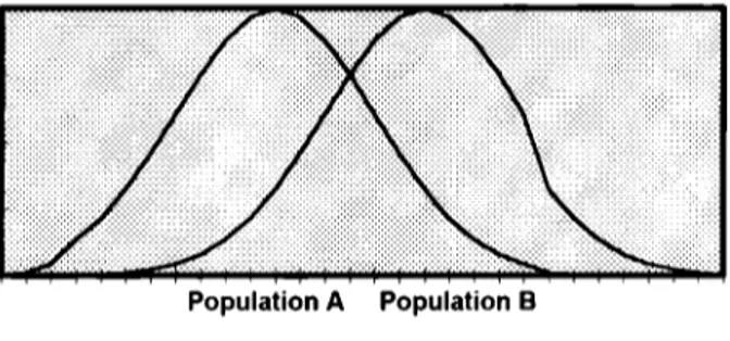
(23) 18. of two brands and a single attribute being evaluated. Figure 1.1 describes the consumer' s perception of a single attribute held in different amounts by the two brands.. Population A. Population B. Figure 1. 1. Overlap between brand densities.. The loyal consumers for brand A are located on the left of the graph, given that B probability density function has minimum area in common with A in this zone, then consumers perceive brands A and B as having a different amount of the same attribute, so the probability of their buying brand B is el ose to zero. A similar situation would be expected for consumers 'loyal' to brand B located on the right. For the consumers in the middle of the graph, the common area represents the degree of similarity among the two brands in terms of the attribute under consideration, so high switching between the two brands is expected. Then the extent of overlap between the two densities can serve as a substitutability index for the brands holding the attribute being evaluated. If the two densities fully overlap, it means consumers perceive identical attribute densities for the two brands. On one hand it could be because they are indeed perfect substitutes,. or on the other hand because consumer evaluation uncertainty. about the true differences. Consequently there are no Joya! consumers. Their selection between brands is done at random. In this case, any consumer has a .5 probability of buying any of the brands in the future, and a .5 chance of being classified as 'Joya!' to brands A or B in terms of his purchasing history..

(24) 19. The extension to more than one attribute, say p,. will correspond to two. multivariate density functions which overlap in a p+ 1 dimensional space, and again the extent of overlap perceived by the consumer with respect to this set of p attributes can be interpreted as the 'degree of substitutability' for the two brands. The larger the overlap, the larger the extent of similarity between the brands and therefore more switching between brands is expected.. It is important to notice that for multi-attribute settings, effective overlap depends on the attributes under consideration, and mainly on the weights consumers assign to those attributes. Considering only two attributes, two brands can be 'very' similar in respect to one, but perceived as different in respect to the other. If both attributes are important to the consumer, then there is a chance of driving his choice to one of the brands by heavily promoting the attribute that the brand possesses in a major degree. On the other hand if brands overlap in ali the important attributes, promotional and pricing strategies could lead to favor one or the other. For example if two brands are perceived as similar in terms of the benefits they provide, and one of the brands increases its price, consumers will switch to the other brand because they will see no reason to pay a premium for the same set of benefits. Finally, since the weights assigned to attributes are critica! for meaningful overlap, if brands are similar in respect to unimportant attributes, this will not be relevant in terms of opportunity for differentiation The set of essential attributes to be used as the basis for comparing two brands needs to be suggested by good theory and information about the particular characteristics of the brands under consideration, or after profiling their segments. One this is done, the next step is to assess the amount of overlap (degree of substitutability) between the brands and then to identify those attributes which lead to the minimum extent of overlap between the brands because they represent opportunities for differentiation. Then, the amount of overlap between the probability density functions.

(25) 20. defined by a set of attributes will help to answer the two research questions proposed at the beginning of this chapter:. 1. The larger the amount of overlap, the larger the perceived substitutability between the brands and therefore more switching and closer competence is expected. 2. Those attributes for which the amount of overlap is minimized define the attribute bundle which leads to the maximum separation between brand probability density functions, and therefore represents an opportunity to differentiate the two brands and to drive the consumer brand choice.. The main objective of this work is to extend the information provided by the methods of market structure by providing a means to measure the degree of overlap of brands in respect to a selected bundle of brand attribute dimensions. This provides a way to define what are the set of dimensions which make them to be perceived as close substitutes by the consumers in the segment they serve. Once a subset of competing brands is identified, the demographic and benefit characteristics for consumers can be used to define the segment profile: those attributes which cause brands to highly overlap can be interpreted as the more valuable ones for consumers in that segment. They make up the set of essential attributes which lead to consistency switches among brands in the segment. lt is expected that a different set of attributes would make brands 'overlap' in other segments, confirming in this way why brands are grouped together in different sets. lf the set of attributes which overlap differs, then a single brand can appear in various segments, depending on the dimensions which are mostly appreciated by the consumers in the segment where it is considered Defining substitutability in terms of overlap between two probability density functions, then the problem to be addressed in this work is formulated as follows: Let :((x) be the probability density function defined by a p-vector of x consumer characteristics (benefits sought or product attributes) for the brand i (i=l,2).

(26) 21. 1. Identify the fundamental reasons for the separability of the two densities in terms of the density moments, or by computing proper separability measures. 2 Construct a discrimination function [h(x)] that maximizes class separability in the reduced space where h(x) is defined. 3. Estímate the total error associated with the discriminant funcion h(x). This error is a surrogate measure for overlap in the discriminant space. lt will be important at this stage to asssess the quality of this overlap measure, because it will depend on the assumptions about the conditional densities f(x). 4. Relate this error to the degree of substitutability between the two brands with respect to the p attributes considered in the x vector, and if appropriate, compare the val u es of this substitutability index for severa! bundles of p attributes The general problem of constructing a function so that separation among g groups is maximized, corresponds to the statistical methodology known as Discriminant Analysis. Once the discrimination function is constructed, the best way to evaluate its efficiency is to compute the associated misclassification error rates, which correspond to the sum of the conditional probabilities for misclassification, namely, for two groups:. Total error= P(allocate to group 11 x. E. group 2) + P(allocatc to group 21 x. E. group 1). This total error rate can be viewed as the amount of overlap between the two densities but measured indirectly in the reduced space corresponding to h(x), the discriminant rule. The situation is depicted in the Figure 1.2..

(27) 22. Pr (allocate to 1 1 2). Pr(allocate to 2 11). Figure 1.2. Relation between overlap and conditional error rates.. Based on the above formulation for the problem, this work propases to measure the extent of overlap in the multivariate case via the methodology of Discriminant Analysis. The rest of this work is organized in four chapters. The second chapter provides a discussion about overlap measures reported in the literature for the unidimensional case, as well as an assessment about the impact of the density function characteristics and the sample size on the extent of overlap. Chapter 3 is intended to support the selection of error rates for discriminant function as measures of densities overlap. This chapter describes, in general, how to construct a discriminant rule and how to estímate its associated error rate. The main interests are: separability measures, the optimality of linear discriminant functions and the quality of estimation methods for error rates. Chapter 4 develops a procedure to construct a linear discriminant function, by using the so called Disco coefficient suggested by Guttman (1988) as the separability criteria. The procedure considers the case of only two brands competing in a segment, and a 2-attribute set under study. The value of the Disco coefficient is proposed as an index of substitutability for the two brands, because it is related to the extent of similarity in attributes ( overlap) for the two brands. This chapter also presents the computational implementation required to find the proper attribute weights for a linear discriminant function, as well as the evaluation of the multivariate disco criterion by bootstrap methods. Finally, Chapter 5 presents the conclusions, drawbacks, and directions for future research derived from this work..

(28) 23. CHAPTER 2. OVERLAP BETWEEN GROUPS IN THE UNIVARIA TE CASE.. The discussion in this and the following chapters is restricted to only two groups under study. This chapter is focused on the univariate case, namely, only one characteristic is used to assess the separability between groups. The first section relates overlap to a mean difference, and in particular to the usual practice of comparing group meaos and taking the test significance as evidence for good separation. The second section presents the overlap measures reported in the Social Sciences literature and their drawbacks and relation to true overlap. Since overlap percent is a function of the true underlying probability distributions, normal densities were assumed for these two sections. This assumption allows for simpler computations and is also a very common assumption for practitioners. The third section shows how overlap is determined not only by a difference between means but also by differences in variability and skewness in the group distributions. Skewed distributions from the gamma family are used in this section to illustrate how overlap can be very high when non-normal data are under study.. 2.1. Hypothesis comparing group meaos and its relation to the extent of overlap.. In the univariate case, a parametric approach used to compare two populations is that of testing statistical hypothesis in respect of their means and variances The usual parametric tests involve t-Student and F, to test equality between means and variances respectively. When the assumption of only a finite vector of unknown parameters for a specified probability distribution is not valid, methods with less stringent assumptions are applied. But even in the non-parametric case, assumptions, as 'the same continuous probability distribution', are imposed so that the test can be formulated as one about different location for the two distributions, as is the case of.

(29) 24. Wilcoxon or Mann-Whitney tests (Conover, 1981 ). If the purpose of the statistical test is limited to show equality in location parameters for the distributions, the named tests are appropriate. But if a parametric test rejects the hypothesis about equality of means, this cannot be taken as evidence for good separation between populations. Means can be declared statistically different, but populations involved can still have a high extent of overlap. The separation between means is just an evidence that a linear allocation rule (see next chapter) can be constructed, but even in the case of good separation between means, the resulting classification rule could be inappropriate, in the sense of a high misclassification error associated with the populations overlap. Considering the case of the commonly used t-test, it involves the computation ofthe sample means difference in units of the corresponding standard deviation. Given that the sample means are consistent statistics, good separation between the sampling distribution for the arithmetic means is always possible: as the sample size increases, power will increase and eventually will lead to a significant test, even when actual probability distributions highly overlap. To illustrate this situation a set of tables and graphs was constructed, under the usual assumptions of two normal distributions with equal variances which lead to a ttest. The homoscedasticity assumption will allow to handle the extent of overlap only as a function of the distribution means. More general results will be given in the next section. In the construction of the following tables and graphs, (without loss of generality) unit variance is assumed for the two densities, the difference between the population means (8) is given as a multiple of the standard deviation which under the assumption of cr=l would be equivalent to the raw difference As mentioned at the end of the first chapter, overlap is defined as the common area for two continuous probability distributions. Since normality is assumed, the extent of this area (overlap) can be computed by using the standard-normal distribution and noting that overlap would be equal to 2Pr(Z>8/2). As the separation between means increases, the amount of overlap decreases, resulting in separability between the two densities..

(30) 25. Figure 2. 1. depicts graphically the relation among the concepts of overlap, shared area between the two probability distributions, and the Z-values used to determine the amount of overlap. ~~ µ¡. µ2. Figure 2.1. True extent of overlap for two univariate densities. The power of the t-test for the hypothesis about equality of meaos depends on the true difference between the meaos (and, therefore, from the amount of overlap ), the significance leve) and the sample size. Then to compute this statistical power, the two most commonly used significance levels were employed, namely .05 and .O1. Respect to sample size, the same sample size n was assumed for the two populations under study (then, total sample size is 2n). The values range from 2 to 200. For total sample sizes below 30, the power of the statistical test was computed by using the non-central t-distribution, with the non-centrality parameter given by 11· =. ½. 21. n,. For total sample size above 30, the standard normal distribution was used Computations were performed by using the section on Probability Distributions in the statistical package MINIT AB (1994). Tables 2.1 and 2.2 show. o,. the difference. between populations meaos, the amount of overlap, and the corresponding power for.

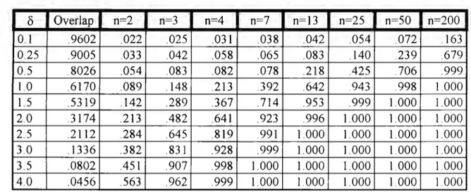
(31) 26. the test for severa! sample sizes. Table 2.1 is constructed by using 05 as significance leve!, and Table 2.2. by using .01. The entries in the tables stand for the corresponding power ofthe t-Student test with 2(n-l) degrees offreedom. Table 2.1. Relation between overlap and statistical power under a=.05 (). 0.1 0.25 0.5 1.0 1.5 2.0 2.5 3.0 3.5 4.0. Overlap .9602 .9005 .8026 .6170 .5319 .3174 .2112 .1336 .0802 .0456. n=2 .022 .033 .054 .089 .142 .213 .284 .382 .451 .563. n=3 .025 .042 .083 .148 .289 .482 .645 .831 .907 .962. n=4 .031 .058 .082 .213 .367 .641 .819 .928 .998 .999. n=7 .038 .065 .078 392 .714 .923 .991 .999 1.000 1.000. n=13 .042 .083 .218 .642 .953 .996 1.000 1.000 1.000 1.000. n=25 .054 .140 .425 .943 .999 1.000 1.000 1.000 1.000 1.000. n=50 .072 239 .706 .998 1.000 1.000 1.000 1.000 1.000 1.000. n=200 .163 .679 .999 1.000 1.000 1.000 1.000 1.000 1.000 1.000. Table 2.2 Relation between overlap and statistical power under a= O1 (). 0.1 0.25 0.5 1.0 1.5 2.0 2.5 3.0 3.5 4.0. Overlap .9602 9005 .8026 .6170 .5319 .3174 .2112 .1336 .0802 .0456. n=2 .005 .008 .012 .023 .033 .047 .092 . 118 .153 .221. n=3 .006 .013 .018 .045 .093 .184 .262 .384 .539 .633. n=4 .007 .011 .025 .073 .152 .303 .462 .629 .941 .982. n=7 .008 .014 .025 .164 .422 .677 .921 .983 .998 .999. n=13 009 .025 .075 .392 .814 .976 .999 1.000 1.000 1.000. n=25 .024 .075 .289 .887 .999 1.000 1.000 1.000 1.000 1.000. n=50 034 141 .432 996 1.000 1.000 1.000 1.000 1000 1000. n=200 075 .455 .992 1000 1.000 1.000 1 000 1.000 1.000 1.000. By using the data from these two tables, the graphs in Figures 2.2 and 2.3 were constructed. By means of these graphs one can appreciate that the power of the test is high, even for a large extent of overlap as long as the sample size is large enough.

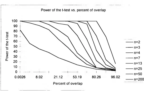
(32) 27. Power of the t-test vs. percent of overlap 100 ' 90 -. 1. --..... 80 70 60 ~ 50 -'-. (/). Q) 1. Q). .r::.. --n=2. 1. '+-. o. --n=3. 40 -· 30 1 20 -;-. Q). ~. o. (l_. --n=4 --n=7. --n=13. 1O -:. o. --n=25. ' ---1. 1. 0.0026. -1--. 8.02. 1. --+----1-. 21.12. 53.19. --n=50 80.26. 96.02. --n=200. Percent of overlap. Figure 2.2. Relation between percent of overlap and power of a t-test, a= O.OS. Power of the t-test vs. percent of overlap 100 90. --.... ( /). Q). 80 70. 1. Q). 60 -. ' +-. 50 -. .r::.. o. Q). ~. o. (l_. --n=2. 40. --n=3. 30 --. --n=4. 20. --n=7 --n=13. 0 --- --1--+. 0.0026. 8.02. 21.12. 53.19. Percent of overlap. 80.26. 96.02. .--n=25 , __ n= 0 5 --n=200 ·. Figure 2.3. Relation between percent of overlap and power of a t-test, a= 0.01..

(33) 28. For example, for a 53.19 % of overlap (more than half of the total area below a density ), the power is abo ve .70 for a total sample size of 14. This implies that a mean difference will be declared 70% of the time even when the two densities under consideration overlap in more than 50%. Only when very small sample sizes, namely 2, 3 and 4, are considered, the amount of overlap needs to be very low (below 30%) to have a significant test. As expected, when the significance level is O. O1, the power of the test decreases, and it drops severely for small sample sizes, but even for this astringent level, a total sample size above 26 (n=l3) is large enough to get a power above .80 when the extent of overlap is 53.19%. As discussed in the paper by Sawyer and Ball ( 1981 ), studies in marketing usually involve large sample sizes, resulting in statistical power over 80% to detect a medium size effect. Sawyer and Ball mainly discuss a casual relation for two variables (regression analysis), and they point out that a significant test cannot be taken as evidence of a high proportion of explained variance for the dependent variable. The authors provide sorne examples where power of the test was large enough to detect small factor effects, even though the proportion of variance explained by these significant factors was very low. In a similar manner, for the t-test under discussion, given a sufficiently large sample size, it is expected to declare a difference between means, but this result will not be sufficient to assure good separation between the original populations, nor a chance to classify elements in one or another group in terms of the single attribute used to compare the means. As a result, in arder to assess the degree of separability between the two probability density functions, a reliable measure for the extent of overlap or group separability would be required, besides the significant t-test..

(34) 29. 2.2. Overlap measures in the univariate case.. Since the extent of overlap is directly related to the standardized meaos difference (8 in the tables and graphs ), it is not surprising that one of the earliest measures proposed to assess the extent of overlap was the standardized meaos difference suggested by Tilton ( 193 7), who defined overlap as "the percentage of area common to the two distributions". Tilton's D measure is computed by the following plug-in sample estimator:. (1). where sP stands for the pooled standard deviation, the square root of the pooled sample variances. D=O when there is 100% overlap, and it will increase as the separation between population meaos increases. For this measure, class separability is given as a function of the standardized meaos difference. For symmetric distributions with the same variance, D will decrease as the meaos distance decreases, or when the variance increases, thus providing a measure which monotonically decreases as overlap increases. Assumptions regarding the true underlying distributions will be required to determine the true relation between overlap and D. If the two populations do not have the same variance, the use of the pooled variance (.\'P) in the denominator will decrease. D as the two variances ratio increases for a constant meaos ditference. This behavior for D is satisfactory, because, as it will be shown in section 2.3,. overlap between. distributions increases if the variance of at least one of them <loes. Another early univariate measure for the extent of overlap was suggested by Symonds ( 1930), and defined as the percentage of one distribution reaching or exceeding the median score of the other ( distribution.) This measure always underestimates the true extent of overlap because it measures only part of the total.

(35) 30. common area, namely the area above ( or below) the median of the other distribution. This situation is depicted in Figure 2.4, where the gray area corresponds to the median overlap measure, and the black area to the total overlap.. Md1. Md2. Figure 2.4. Overlap and its relation to the median proportion measure. Recognizing the bias of the median proportion measure, Symonds (1930) also suggested the biserial correlation coefficient ( r6 or biserial r) as an improved measure ofthe extent of overlap. For two normal densities with a common and known variance cr, sample rb is defined as follows:. where p is the proportion of elements with x-scores in the probability distribution with larger mean, and q is the corresponding proportion for the population with smaller mean. u is the common variance for the two populations, and z is the point of intersection between the two underlying densities. For the special case of normal densities, the intersection point z is the ordinate of the normal curve at the midpoint between means and can be obtained from statistical tables. Symonds reported curves and graphs which related the extent of overlap (as the area of one density above the.

(36) 31. mean of the other density) with the biserial r values: as the amount of overlap decreases, rb decreases for p=q= 112, (prior probabilities of belonging to any class are assumed to be the same.) Symonds also reported tables which relate rb between groups to the probability that an individual with a x-score located at certain distance above the mean of one group will belong to that group rather than to the other one. As expected, the probability of belonging to the group with the higher mean increases with the direeted distanee of the x-seore to the global mean (meaning x-seore is a high value), but probabilities also inerease with the biserial r val u es, meaning that larger separation (less overlap) between distributions leads to better alloeation for a new xseore. The proportionality relation between biserial r and percent overlap reported by Symonds, was regarded suspiciously by Tilton (1937), and, in a later study, investigated more elosely by Alf and Abrahms (1968). They reeognized that diffieulties with rb result from the assumptions underlying the tables eonstrueted by Symonds. The eorresponding assumptions are given as follows: biserial r is an estimate of the produet-moment correlation between a eontinuous variable (normally distributed), and a diehotomized variable whieh has an underlying normal distribution. Symonds assumed that the eontinuous variable (the x-seores) is always normal within eaeh group regardless of its membership, then for rb = 1, the Symonds' classifieation se heme will be the same as forming two groups, one for the seores above the mean of the xseores, and the other for seores below the mean. This is a naive classifieation rule Alf and Abrahms determined the relation among rb , the pereent of overlap and Tilton's D, to be the following:. ¾overlap. sin -i rb. =------.9. (3).

(37) 32. from the above relations, they concluded that rh subestimates the extent of overlap. Considering a bivariate probability distribution and a linear relation between the two variables involved, Alf and Abrahms derived an improved measure for overlap, the point biserial correlation coefficient, defined as. Pph. =. µ 1 -µ 2. Jpcj. (4). Cft. where µ¡ is the mean of the predictor variable corresponding to the i-th dichotomized value of the other variable; p and q the prior probabilities for groups 1 and 2 respectively; and. CT I. the standard deviation of the combined groups. If p=q, and. groups 1 and 2, are normally distributed with the same variance, Alf and Abrahms give the next relations among the standardized mean difference, point biserial correlation , and the area percent overlap:. P pb. = µ1 - µ2 = D 2CT. (5). 2. Percent overlap = <l.J(D/2), where <l.J(.) stands for the standard normal distribution function.. The relationship between point biserial correlation and percent overlap will be dependent on the x-score distribution; therefore, a general relation cannot be derived. Figure 2. 5 shows the relation between percent overlap and the corresponding biserial and point biserial correlation values under the assumptions of normality, homoscedasticity and equal group probabilities. Percent overlap and. biserial. correlation values have a curvilinear relation, where the values increase slowly once.

(38) 33. the overlap is below 40%. Values for the biserial correlation around O. 9 -which will be considered highly significant for a correlation coefficient- occur when the percent of overlap is around 30. The graph resembles the relation between power of the t-test comparing group means and percent of overlap, and allows to conclude that even for distributions with a moderate extent of overlap (30-40%), one can get a significant ttest and a high biserial correlation. Therefore, these results need to be interpreted with caution if the final objective is to define separability between two groups and the opportunity to correctly allocate new elements.. 0.8 CII. i. ·u. 0.7. !i: GI o CJ. e. - - biserii coefficient. ~ra 0.5. .. !! 8. -1. 1- - point biseri~I coefficient ,. 0.4. ii. ·;:. 5: 0.3 :.e 0.2 0.1. o 10. 20. 30. 40. 50. 60. 70. 80. 90. 99. percent of overlap. Figure 2. 5 Relation between percent of overlap and biserial correlation coefficients.. The second graph in Figure 2.5, corresponds to the point biserial correlation. The relation is approximately linear, with values over 0.9 only if the percent of overlap is less than 5. Sin ce p pb is directly related to the extent of overlap and Tilton' s D, it is.

(39) 34. a better measure. Figure 2.5 was constructed by using the values reported by Alf and Abrahms, these results assume that the true parameters are known, so the performance of p pb under sampling is expected to be less satisfactory. More recent measures of the extent of overlap in the univariate case were recently proposed by Guttman ( 1988) in relation of two groups.. In order to define the two overlap coefficients, let x be the value of the numerical variable used to classify individuals. If two independent samples of size n are taken from each of two populations, A and B, denote by x P the corresponding x-value for individual p in population A, and by xq the x-value for individual e¡ in population. B. Let xA and xEJ be the corresponding sample means, then define the next relation. UAH = ¿¿(xp -xq)(xA -xB). (6). pe A qc 11. Perfect discrimination ( no overlap) occurs if for ali p and e¡, the x" values from population A exceed the xq values from population B given that This latter condition is equivalent to. vAH. lx" - xq 1= x" -. = LLlxp -xql(xA -x1J. x11. is greater than. x11 .. xq , thus define v AB as follows:. (7). p, A q•.11. Then to discriminate individuals from populations A and B define the Disco coefficient as u AH /v AH . Guttman showed that the values of the coefficient are always between O and 1, with zero meaning complete overlap and one perfect discrimination. If the coefficient attains its maximum value of one, there is no overlap between groups A and B, because the so named DISCO condition holds. The condition is given by. max. (xlb) s; min(xla). (8).

(40) 35. The Odisco coefficient is a relaxed overlap measure. For this coefficient the meaningful comparison is versus the sample means, then define the next relations. u;8 = 2¿(xp -xA)(xA -xu). and v;B =. 2¿1xp -.XAl(X/1 -XB). (9). pEA. pEA. and the odisco coefficient as the corresponding quotient between the above summations. Perfect discrimination occurs under this relaxed condition only if the odisco coefficient attains the value one. Here overlap is allowed, because if the next relation holds for the two population means. then odisco coefficient will be one provided the next condition holds. max(xjb) ~ µA,. min(xla) ~ µ 8. (10). Condition ( 1O) is called O DISCO condition. Guttman shows that the next relation holds between the two coefficients used to assess overlap:. º < *A/J / * < - U. V Ali - U AB / VAH. <l -. (11). These two coefficients are non-parametric. Their relation with the percent of overlap is not given in the paper by Guttman. It is important to note that both coefficients measure overlap as a means difference, because only the first moment is involved in their computation, therefore they will represent a proper overlap measure only for the case of symmetric distributions with the same variance..

(41) 36. To study the relation between the percent of overlap and the Disco and Odisco coefficients under sampling, a series of experiments was performed In total, 17 random samples of different sizes from 7 to 100 (the same sizes used with the power graphs ), were generated from two normal densities, both with variance equal to one, by using the random number program from MINIT AB. The parent populations differed only with respect to the location parameter (see comment at the end of previous paragraph). Four distances between density means were used, the separation between means corresponds to 90.05, 80.26, 61. 70 and 31. 74% of overlap. Only for sample size n=7, a greater separation between means was tested (3. O units or equivalent to 13. 36% overlap ), because the val u e of the coefficients for ali other sample sizes is almost one for higher distances. Computations showed that no significant difference occurs in the coefficient values above a two-unit distance. Table 2.3 shows the mean, standard deviation and coefficient of variation for the Disco and Odisco coefficients computed from 25 trials at each sample size and means distance combination. Computation of the coefficients was performed by using a BASIC program written for this purpose.. Table 2.3. DISCO and ODISCO coefficients under simple random sampling. SAMPLE SIZE (n) n=7 Disco ES (disco) CV (disco) Odisco ES (odisco) CV (odisco). 0.25 0.340140 0.266241 78.27 0.439999 0.313007 71.14. 6 = means distance (in standard deviations) 1.00 2.00 3.00 O.SO 0.997822 0.802742 0.959022 0.397443 0.094933 0.004192 0.286611 0.088656 0.42 72.11 44.68 9.91 0.999999 0.757479 0.982560 0.457464 3.354 xE-05 0.309911 0.052296 0.319642 0.0034 5.32 69.87 40.91.

(42) 37. Table 2.3. DISCO and ODISCO coefficients under simple random sampling. SAMPLE SIZE (n) n=l3 Disco ES (disco) CV (disco) Odisco ES (odisco) CV (odisco). o= means distance (in standard deviations) 0.25 0.50 1.00 2.00 0.2406001 0.354078 0.659689 0.968578 0.19682 0.185780 0.258149 0.030185 81.8 52.47 39.13 3.12 0.30494 0.782468 0.466611 0.998467 0.25775 0.215878 0.229516 3. 069(E-03) 84.52 46.27 29.33 0.31. n=25 Disco ES (disco) CV (disco) Odisco ES (odisco) CV (odisco). 0.25. n=50 Disco ES (disco) CV (disco) Odisco ES (odisco) CV (odisco). 0.25. n=l00 Disco ES (disco) CV (disco) Odisco ES (odisco) CV (odisco). 0.25. 0.50. 0.205289 0.161374 78.60 0.2777578 0.205797 74.14. 0.365820 0.149879 40.97 0.484498 0.191646 39.56 0.50. 0.31761 0.101611 31.99 0.43142 0.133745 31.01. 2.00 0.770867 0.098913 12.83 0.904733 0.068039 7 52. 1.00. 0.419822 0.124560 29.67 0.554089 0.161608 29.17 0.50. 0.220633 0.067772 30.72 0.307833 0.091913 29.86. 1.00. 2.00 0.728322 0.085057 11.68 O 845978 0.89901 10.63. 1.00 0.422256 0.058091 13.76 0.560733 0.070307 12.54. 0.963844 0.25157 2.61 0.963856 0.025165 2.61. 0.961544 0.018760 1.95 0.995001 5.715(E-03) 0.57 2.00. 0.709611 0.067486 9.51 0.852467 0.055337 6.49. 0.954522 0.014307 1.50 0.991644 4.230(E-03) .43.

(43) 38. As it was expected, the value of the coefficients increases as the separation between means increases and the percent of overlap decreases. Unfortunately, the variability in the coefficients is very high for small sample sizes, even in those cases with large overlap. The coefficients of variation are above 70% when means distance is O. 25 units and sample size is as small as 7, 13, and 25; and they are abo ve 3 0% when means distance equal or below 1. O for sample sizes under 25. For larger sample sizes, namely 50 and 100, the variability decreases notably; with acceptable values (below 30%) for moderate (1.0 unit, equivalent to 61.7% overlap ), and large means distance (2. O units, equivalent to 31. 7 4% overlap ). Very low variability and values near to one occur when there is large separation between means, independently of the sample size. Even for n=7, values of the coefficient rapidly converge to one as the extent of overlap decreases. From these results one can conclude that the disco and odisea coefficients are a reliable measure of overlap if the sample size is large enough or if the separation between population means is of at least one standard deviation. Then if a significant t-test is obtained -meaning population means are well separated- the Disco and Odisea coefficients would provide a relevant measure for the percent of overlap. Ali the results provided in the graphs and tables of this section were constructed assuming normality. Since ali the coefficients used to measure overlap (biserial, point-biserial, disco and odisea) depend on the true underlying distribution, differences in the results provided could occur for other distributions, in particular for those distributions which differ considerably from the normal. To provide sorne insight on the behavior of these overlap coefficients, when distributions differ not only with respect to the location parameters, disco values were computed for a series of experiments where the parent distribution was non-normal. Results are provided in the following section..

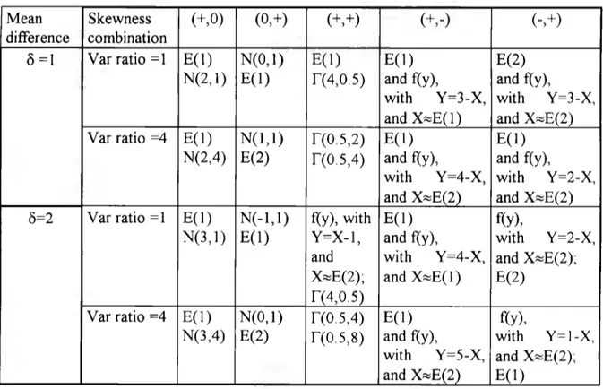
(44) 39. 2.3. Overlap as a function of the first three moments of a probability distribution.. As was mentioned before in this chapter, the difference between means seems to be the main concern for researchers and practitioners when comparing two distributions and in particular two brands respect to a given attribute. But separability between groups depends also on other distribution properties. In order to explore the effect that higher order moments have on the extent of overlap between two distributions, a factorial experiment in three factors was designed. The factors under study were the following:. A= Mean difference, with two levels 8 = 1, and 2 (not standardized) B = Variance ratio, with two levels cr 1/cr 2 = 1, and 2, C = Skewness combination, with five levels represented as pairs of distributions which could be symmetric (skewness represented by 'O'), right skewed (+), or left skewed (-). Levels: (+,O) (O,+)(+,+)(+,-)(-,+). Since the ratio and mean difference for two distributions can assume any real positive value, factors A and B were considered random, while factor C was assumed fixed because its levels correspond to ali possible combinations of skewed distributions. The (-,-) combination was not considered because it is equivalent to the. (+,+) for the particular purpose of measuring overlap. The skewed distributions were ali members of the gamma family, and proper transformations were done to provide left skewed distributions. The gamma family was selected because this distribution is frequently used to model data for Marketing and Engineering models, and it was also a convenient choice given the available software. Table 2.4 reports the two distributions used to represent each particular combination of the three factors under study, namely: means difference (8), ratiovar,.

(45) 40. and skewness combination. For example, for the first cell in the table, the distributions are: E( 1), which corresponds to the exponential distribution with expected value equal 1; and N(2, 1), which states for the normal distribution with mean 2, and variance equal 1. F or this combination, the difference between means is 6= 1 (2-1 ), and both distributions have the same standard deviation (cr=l ), i.e. ratiovar=l. The first distribution is positively skewed, with a skewness coefficient equal S = +2, while the normal density is symmetric, with S = O. Then the distributions correspond to the skewness combination (+,O). As another example, take the last cell in the table. The two corresponding densities are: f(y), a continuous density function for the random variable (r.v.) Y. Where Y=l-X, i.e. Y is a transformation from an exponential random variable (X), the expected value of X is 2, and the one for Y is -1. The other distribution is an exponential density with expected value equal 1. In this case, since the mean of the first variable is -1, and the mean for the second r. v. is 1, then 6=2. Variance of first distribution is 1, and for the second four, then ratiovar=4. Finally, f(y) is a density skewed to the left, and the exponential E( 1) is skewed to the right, providing the combination (-,+). Finally, The notation r(a,~) which appears in sorne other cells corresponds to the gamma density with parameters a, ~For a particular pair choice, a unique overlap percentage is defined. Therefore, the variability in the overlap percentage will come from the infinite number of possible distributions that can be selected to represent each factor combination. For each experiment, the true overlap was computed following two steps: 1. Compute the intersection point between the two probability density curves by using the specialized mathematical software "Mathematica" ( 1991 ), or by hand in those cases where it is possible. 2. Compute the true overlap as the shared area between the two densities. These computations were all done by using MINIT AB..