Economic Growth and Income Distribution

Texto completo

(1)ECONOMIC GROWTH AND INCOME DISTRIBUTION BY MACARIO SCHETTINO YAÑEZ. APPROVED. SUPERVISOR_ _ _ _ _ _ _ _ _ _ _ _ _ _ _ _ __ Leslie Young University of Texas at Austin Carlos Urzúa ITESM/El Colegio de México José Romero ITESM/El Colegio de México.

(2) ECONOMIC GROWTH ANO INCOME DISTRIBUTION.. BY MACARIO SCHETTINO YAÑEZ. A DISSERTATION SUBMITTED TO INSTITUTO TECNOLOGICO Y DE ESTUDIOS SUPERIORES DE MONTERREY IN PARTIAL FULFILLMENT OF THE REQUIREMENTS FOR THE DEGREE OF DOCTOR OF PHILOSOPHY. AUGUST, 1993.

(3) ABSTRACT. ECONOMIC GROWTH AND INCOME DISTRIBUTION. by. MACARIO SCHETTINO YAÑ'EZ. SUPERVISING PROFESSOR: LESLIE YOUNG. Recent theoretical advances in economic growth theory and the empirical studies that followed suggest that it is possible to answer the question:. "What is. the relation. between economic growth and income distribution?" In this dissertation, answers to this question are developed using a function that describes income distribution in a model of. economic _gro_~t:h.. previous. The. resul ts. theoretical and empirical. are. consistent. findings.. wi th. In certain. circumstances, income distribution will reduce the rate of growth_;. also,. under other special circumstances,. income. redistributions may accelerate the economy. Finally, as a general statement,. the less egalitarian the distribution. of income, the lower the rate of optimal growth..

(4) TABLE OF CONTENTS Page ECONOMIC GROWTH AND INCOME DISTRIBUTION ................. i ACKNOWLEDGMENTS ........................................ i v LIST OF ILLUSTRATIONS ................................... v LIs T o F TABLE s . . . . . . . . . . . . . . . . . . . . . . . . . . . . . . . . . . . . . . . . . Vi INTRODUCTION ............................................ 7 PART I. CHAPTER 1. THE DESIRABILITY OF ECONOMIC GROWTH. ECONOMIC GROWTH ............................. 11. I. Economic Growth or Economic Development? ............ ·11I I . Economic Growth .................................... 1 7 CHAPTER 2. INCOME DISTRIBUTION ......................... 33. I. Income Distribution Measurement ..................... 33 II. Income Distribution and Demographic Factors ........ 38 III. Income Distribution and Economic Growth ........... 42 PART II ECONOMIC GROWTH ANO INCOME DISTRIBUTION. CHAPTER 3. AN OVERLAPPING GENERATIONS MODEL ............ 45. I. The Model ........................................... 45 I I. Economic Equilibrium ............................... 4 7 III. Political Equilibrium ............................. 48 IV. Dynamics of Growth .'. :'· • ............................. SO.

(5) V. Minimal Consumption .....•...•.............•.......•• 51 CEAPTER 4. APPROXIMATING THE LORENZ CURVE . . • . . . . . . . . . . . 57. I. The Function . • • . • . . • . • . . . . . . . . . . . . . . . . . . . . . . . . . . . . . . 57 II. Em.pirical Results . . . . • • . • . . . . . . • . . . . . . . . . . . . . . . . . . . 60 III. Cros·s-Country and Time-Series ..•..••.............. 64 CHAPTER 5. EXOGENOUS GROWTH ANO INCOME OISTRIBUTION ...• 77. I. A Simple Model ••.•..•......•.••....•.•...••..••...•• 77 II. Oynamics of Income Oistribution •.••••.••••••.••.•.. 89 III. Empirical results •••••••••••••••••••••••••.••••.•. 99 APPENOIX TO CHAPTER 5 ••••••••••••••••••••.••••••.••.•• 102 CHAPTER 6. ENOOGENOUS GROWTH ANO INCOME OISTRIBUTION •• 104. CHAPTER 7. CONCLUS I ONS • • . • • • • • • • • • • • • . • • • • • • • • • • • • • . • • 114. BIBLIOGRAPHY . . . . . . . . . . . . . . . . . . . . . . . . . . . . . . . . . . . . . . . . . . 118. iv.

(6) LIST OF ILLUSTRATIONS ~igure. Page. Figure l. l. Technological Progress ................... 21 ~igure 2.1. ?overty and Income Distribution .......... 35 rigure 3.1. Minimal Consumption and Capital Restriction . . . . . . . . . . . . . . . . . . . . . . . . . . . . . . . . . . . . . . . . . . 54 Figure 3.2. Arnount of Poverty and minimal redistribution tax . . . . . . . . . . . . . . . . . . . . . . . . . . . . . . . . . . . 55 Figure 4 .1. Lorenz curves . . . . . . . . . . . . . . . . . . . . . . . . . . . . 7 4 Figure 4. 2. First Decile . . . . . . . . . . . . . . . . . . . . . . . . . . . . . 74 Figure 4.3. Middle of the curves ..................... 75 Figure 4. 4. Top of the distribution .................. 75 Figure 4. 5. Absolute Residuals ....................... 76 Figure 4.6. Relative Residuals ....................... 76 Figure 4. 7. Relative Residuals ....................... 77 Figure 5.1. Response of Figure 5. 2.. M;. 0'¡ 01. to a and b. . ............ 92. and Gini coeff icient .................. 97. Figure 5.3. Income Distribution and Growth ........... 98 Figure 5.4. Income Distribution and Growth ........... 99 Figure 5. 5. Income and Distribution. Parameter a .... 102 Figure 5.6. Income and Distribution. Parameter. V. P ..... 102.

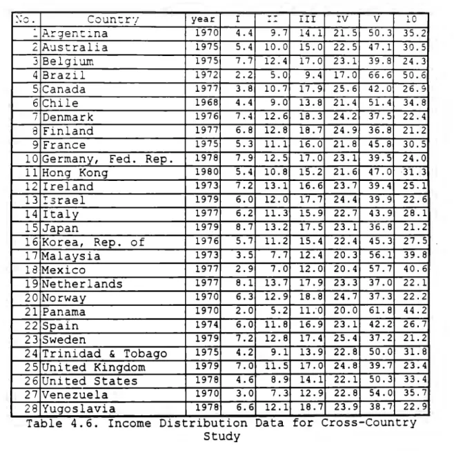
(7) LIST OF TABLES Table. Page. Table 2.1. Inequality Measures ....................... 38 Table 4.1. Estimation Results and Comparison with Basmann et al ........................................ 6 6 Table 4.1. Estimation Results and Comparison with Basmann et al.. (Cont.) ............................... 67. Table 4.1. Estimation Results and Comparison with Basmann et al.. (Cont.) ............................... 68. Table 4. 2. Sum of Squared Residuals ................ ·.. 68 Table 4.3. Non-linear Regression results ............. ·69 Table 4. 4. Linear Regression resul ts ................. 69 Table 4.5. Robustness of Linear Regressions .......... 70 Table 4.6. Income Distribution Data for Cross-Country s t ud y . . . . . . . . . . . . . . . . . . . . . . . . . . . . . . . . . . . . . . . . . . . . . . . . 71. Table 4.7. a, 13 and y for different countries ........ 72 Table 4.8. Income Distribution Data far Mexico. 19501989 . . . . . . . . . . . . . . . . . . . . . . . . . . . . . . . . . . . . . . . . . . . . . . . . . 73. Table 4. 9. a, 13 and y for Mexico ..................... 73 Table 5.1. Cross Country results .................... 101. vi.

(8) INTRODUCTION. The. question. economic. growth. distribution. of and. has. whether at. been. economic development. economic gives. growth,. us. a. country. same. time. major. issue. can a. experience. better. in. the. income. field. of. The arrival of the "new school" of. also. hope. the. a. that. called the. endogenous. relationship. growth. between. theory, economic. growth and income distribution may be better understood.. This stated. dissertation in. the. relationship growth. can. be. has. title,. is. between. two. main. objectives.. to. find. out. income. more. distribution. One,. about. and. as the. economic. The other is to show that development economics much. more. experiences.. My. development. theory. than. collection. personal has. hypotheses completely 1 , recognized. a. (Bardhan,. not. impression been. able. of is. to. cases that. and since. formalize. i ts. i ts true importance has not been 1993).. Many. developme~t; __ ~heorists. ··------. have believed that income ine-quality m_a.y_ slow the rate of --------·-·--. :with few, but very important, exceptions. 7.

(9) 8. gro'-v'th of a country,. but until recently,. there has not. been a theoretical effort to show this.. In this dissertation I will develop such a rnodel and show. that. increase. incorne. the. rate. distribution of. growth.. rnay. This. indeed result. reduce. is. or. irnportant. since there is ernpirical evidence of both phenornena, as we shall see later. This thesis has the following structure. In the first two chapters I will review the work that has been done in this field. The first chapter is devoted to econornic. growth,. while. chapter. 2. deals. with. income. distribution.. The core of the dissertation is in chapters three to six. Chapter three presents a model of income distribution and ')(. economic. Tabellini (1992). growth to. which. developed I. by. incorporate. Persson a. and. political. feasibility condition, finding that inequality may be even more harmful than what they present.. Then,. in arder to. find a more formal and overwhelming way to analyze income distribution and economic growth,. I. dev~Jo_p__ in chapter. four a function that fits the Lorenz curve and has sorne interesting theoretical and empirical properties.. 8.

(10) 9. In chapter five I develop a model of economic growth including a function of income distribution that responds t~ changes in income.. sorne. ir.teresting. process.. Once. The solution to this model presents. insights. we. have. into. found. the the. economic way. in. development. which. income ,/. distribution. depends. on. the. economic. variables,. describe the process that growth will follow, possible. to. distribution, point. of. the. show. that. the. less. we. and it. egalitarian. can is the. the lower the rate of growth. An important model. is. that. by. including. an. income. distribution function we are modeling reality in a better way than it was done before. In chapter six, the model is expanded to include human capital in order to explore more on the relation between distribution and growth.. The conclusions of this dissertation open many paths for future work on the study of the development process. Inequality is harmful for growth,. and it is a result of. institutions. Thus, institutions may be the most important determinants of growth. Surely, underdevelopment is nota matter of income only.. 9.

(11) PART I. THE DESIRABILITY OF ECONOMIC GROWTH. 10.

(12) CHAPTER 1 ECONOMIC GROWTH. This. chapter. deals. diÍference. between. developrnent. is. with. two. econornic. stated,. issues.. growth. pointing. out. First,. and the. the. econornic issue. that. econornic growth by itself rnay not be as useful as it was once. thought.. The. second. part. of. the. chapter. recent advances in econornic growth theory,. surveys. the so called. "new growth theory".. I. Econornic Growth or Econornic Developrnent?. This is a very hard question. Maybe Robert Lucas has given the best answer: Indeed, I suppose this is why we think of "growth" and "developrnent" as distinct fields, with growth theory def ined as those aspects of econornic growth we have sorne understanding of, and developrnent defined as those we don't. (Lucas, 1988, p.13).. It seerns that econornic growth should be a subset of econornic developrnent, since the focus of the forrner is on explaining how nations experience an increase in their per capita incorne, while the rnain issue of the latter is to 11.

(13) !. .2. explain nations. esonomic. why. the. quality. Economic forces. of. growth. determine. life. varies. greatly. focuses. on. explaining. the. rate. of. growth.. among how. Economi.c. development asks why sorne people die of hunger while sorne others drink champagne and drive Jaguars.. A good. operational. definition. growth is given by Kuznets:. of. what. is. economic. "'. We gauge economic growth by the long-term rise in the volume and diversity of final goods, per capita, with sorne attention to sectorial structure and shifts; but exclude cases where such rise was due largely to natural resources made available by advanced technology elsewhere, or was attained in good part by intensified efforts of workers mobilized to involve a rising proportion of the population". (Kuznets, 1988, p.8). Thus,. only the increase in per capita production due. to changes in productivity (either from capital of labor) may be called economic growth. this. Another issue is whether. increase in production is linked to an increase in. welfare.. This becomes more. important the. less developed. the country of reference is. The issue here is if economic growth is really related to "happiness" or "better life" (Dasgupta, 1988, pp.5-8). The idea that more is preferable to. less. is. Kindleberger,. not. uni versally. accepted. now.. (Herrick. and. 1983, p.7). Even the idea of "growth at any.

(14) cost". is. not. so. appealling. nowadays. in. the. affluent. countries, in light of ecological problems.. In fact,. economic growth by itself seems not to be. enough, as many countries have concluded in recent years.. e .ler and Katz report: Economic growth in the 80's in the U.S.A. is associated wi th less benefi ts for the poor. The change was on returns to skill, which represents less manufacturing employees. (Cutler and Katz, 1991, pp. 51-52). This problem has been analyzed by Juhn, Murphy and Pierce + t:J,.~23), who find that returns to skill in the U.S.A. gro¼'. faster than returns to schooling, or any other determinant in wages. Growth,. then,. is not homogeneous for workers,. increasing wage differentials and making less possible the promise that Kuznets mentions: It is plausible to argue that a major driving force in modern economic growth was the promise not only of greater material welfare but also of a more desirable organization of society that growth would, and does, make possible. (Kuznets, 1988, p.29) / It. is. really a. actually makes. this. controversy whether economic growth reorganization of society possible.. Dreze and Sen have their doubts: Incurring the risk of oversimplifying, an increase in GNP per capita may give the opportunity of better.

(15) quality of life. But that opportunity may be seized or not. (Dreze and Sen, 1989, p.181). Nct. everything grows. when. income per capi ta. grows.. Sorne non-economic variables tend not to increase at__ th,e sarn,~_pª~~- as-i..ncome _pe_r ___c ~ a . Li teracy, for example, is positively related to economic growth, but this relation is. far. from perfect. (Dasgupta,. 1988,. p.96).. Cuba,. for. example, has reached almost no illiteracy with an income per capi ta far lower than the Uni ted Sta tes' . Dreze and Sen state: Sorne non-economic variables determine that increases in. real income may not increase fulfillment of basic needs. There are in principle two reasons for this dissonance (between GNP and life quality): GNP measur_e_sl aggregate income, and i ts translation to quali ty of/ life will depend on income distribution. Second, the/ capabilities enjoyed by people depend on command overr commodi ties, but also on public policies on heal th, education, etc. (Dreze and Sen, 1989, p. 178-180)¡ [italics mine, MS]. __J. Even in the case when income distribution becomes more egalitarian with growth,. we cannot be sure that welfare. has improved. Streeten et al. hold that: Growth by itself even egalitarian growth or redistribution from growth -- does not guarantee the satisfaction of basic needs. A distinctive feature of the basic needs approach is that policies must be implemented to ensure a rising and properly distributed. 1. \'.

(16) :s supply of goods, both private and public, if basic needs are to be rnet. (Streeten et al., 1981, p.108). Basic. needs. differ. frorn. country. to. country,. frorn. region to region, even atan individual level we will have differences. in. (Dasgupta,. 1988).. what. we. consider. For exarnple,. to. be. basic. education rnay be,. needs alrnost. surely, a basic need in the United States or in England or Gerrnany, while it is a luxury good in Haiti or Sornalia.. Sorne. authors. even. think. that. associated to a cultural decline, not. consider. as. "good". econornic. growth. is. sornething that we can. (Dasgupta,. 1988,. p.46).. Ohmae. (1989), cornparing Europe, United States and Japan, states that for incornes above 7,000 dollars, sorne similarities in preferences appear. Furthermore, cultural restrictions rnay prevent. the enlargernent of the production possibili ties. frontier; that is, sorne societies rnay opt not to grow in sorne instances, even if technology is available (Dasgupta, 1988, p.41). Sirnilarly, Kuznets states that institutional problerns rnay preclude sorne LCD' s. frorn develo¡,rnent:. land. proper~y, ~nfrastructure, :politj._<::_s. He says [ ... ] While, in principle, all LCD's rnay pe considered developable, it does not follow that they will becorne developed at sorne future date sufficiently close to rnatter. (Kuznets, 1989, p. 72).

(17) Along these. lines,. Dreze and Sen. (1989,. p.183). hold. that there are two approaches to increase general welfare: O::e is. "growth mediated security",. GNP per capi ta are and. in. public. public welfare. security", income the. followed by increases. expenditure programs.. where. the. of. (absolute. The. focus. redistribution,. reallocation. in which increases in. not. other. one. on. public. is. heal th, factors.. in real. etc. They. relative). is. in. "support-led policies. Success hold. income. like. is based on. that. "There. is. empirical evidence that support-led security is better in this. sense",. "support-led. and. use. South. security".. Korea. Mexico. would. as be. an an. example. of. example. of. "growth mediated security".. Support-led security is. Economic growth had i ts high time. income distribution. around. the. accomplished build up. a. sixties,. but. (Turnovsky, theory. really growth with a better. that. nothing. 1992). includes. Now. in it. this is. line. possible. was to. something besides mere. growth. Chenery et al. stated as early as 1974 that it is possible to grow and have a better distribution of income, at least the empirical side said so, On the theoretical side, it is necessary to discard the conceptual separation between optimum growth and distribution policies that lies at the heart of.

(18) tradi tional wel f are economics. p.xiii). Anyway,. we. should. not. need. ( Chenery et al.,. so. many. 197 4,. apologies. for. s~udying growth's relation to income distribution and for¡ f ocus ing on the poor.. As. T.. Schul tz noted in his Nobel/. J. Lecture in 1979,. '. [M]ost of the people in the world are poor, so if ·,,'a\ knew the economics of being poor we would know much of \ the economics that really matters. J. II. Economic Growth. Economic growth has been studied since the beginning of. economy. century,. theory.. and. it. It. is. was. problem. a. still. a. problem. in. the. today.. solving this issue have been very different.. eighteenth Attempts. at. In any case,. the problem is still unsolved. Quite possibly, the period when. economic. growth. occurred between 1955 approaches. the. became and. 1970.. problem At. least. in. economics. two. different. to understand growth collided in what is now. called the Cambridge vs. Cambridge controversy.. Nevertheless, economic. growth. it. was. started. not to. be. until. the. understood. mid-80's in. i ts. that maj or.

(19) components. called. the. Ro~~-~~~. Befare "new. growth. seminal paper on what t:heory,". published. is now. in. 1986,. economic growth was explained mainly by exogenous factors like. technological. progress.. The. discussion,. then,. was. sterile in the sense that no one was actually explaining growth,. 1. but. trying. to. identify the way. in which growth. \. could be studied.. We growth,. can. identify. different. approaches. in terms of how they view the. to. economic. role of physical ---------. -. One of these identifies capital as homogeneous, -v and.builds an aggregate production function (Solow, 1976). c;:ª-pital.. The other ene states that capital is not homogeneous,. and. rej ects the possibili ty of having an aggregate function. The core of the Cambridge controversy lies here and Laing,. 1977;. Sen,. 1979;. Shaw,. 1992).. (Harcourt. Agreement was. impossible in the seventies, but it may be possible in the nineties. identified. The the. "new. growth. epgpgenous. theory" force. far. has,. precisely,. growth. in. the. heterogeneity of labor, knowledge, products, etc.. Let us start with Solow's model of growth 1 • He posits an aggregate production function of the form. :r will follow an argument similar to the one presented by Shaw (1992)..

(20) :9. where national production is denoted by of overall productivity, are. the. leve!,. and. !abo.:.,. the. renders. (2.1),. Differentiating. technical. capital. of. inputs. Y,, A, is an index. rate. etc.. K,. and L,. respectively. at. the. which. country will grow:. º~ \;') Y,. b '+ ~:-. oE(?:i,) l,. A,. oF(K,,L,) k,'. -=-+---- +---aK, ar, r, Y, A,. (1.2). r,. where the dot indicates a time derivative. If factors are paid. to. according. their. marginal. productivity,. (2.2). becomes. Y,. A,. WL, l,. RK, k,. -=-+----+---Y, A, PY, Y, PY, Y,. (l. 3). where W and R are the labor and capital wages. But WL,/PY, is the labor share while RK, /PY, national product.. Then,. is the capital share of. empirically,. it is very easy to. check that an increase in production, what we have called economic growth, can be produced by a similar increase in producti vi ty. (A) ,. or. by. greater. increases. in. labor. or.

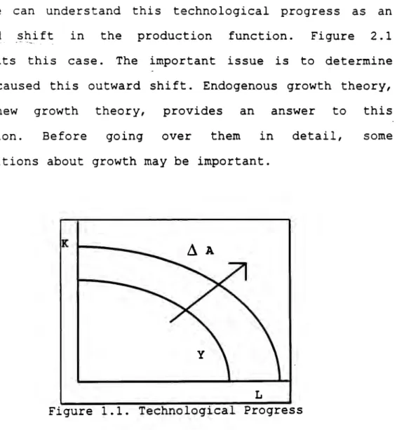
(21) 20. capital.. In fact,. Solow found that for the U.S.A.. period. 1900-1949,. technical. progress,. in the. that. is,. p=oductivity increases, accounted for more than 85% of the total. ir.crease. in. production.. In. short,. exogenous. technological advances explained more than 85% of economic growth.. We. can understand this. upw~_r5=1. shi ft. presents. this. in. the. case.. technological progress. production. The. function.. important issue is. as. Figure. an 2 .1. to determine. what caused this outward shift. Endogenous growth theory, the. new. question.. growth Before. theory, going. provides over. an. them. answer in. to. detail,. definitions about growth may be important.. K. L. Figure 1.1. Technological Progress. this sorne.

(22) 21. A two-fold division is often used to characterize the t:.,-pe o f technological change. When t:echnological progress 1. s. not. as socia ted. "disernbodied". wi th. progress.. the. When,. input:s, on. the. it · is other. called. hand,. it. affects production through the inputs, like new machines, "vintage" capital, etc., it is called "ernbodied" progress.. The other important point to be made about economic growth has to do with the capital/labor ratio. Technical progress is called "Hicks-neutral" if the marginal rate of substitution is unchanged as the progress goes on. In this case, if relative prices do not change, the capital/labor ratio will remain the same. That is the case of equation 2. 1.. I f the progress is not Hicks-neutral,. it. is ei ther. capital-saving or labor-saving.. For each of them, another kind of neutrality has been defined. Harrod-neutrality occurs when the capital/output ----------·· -· --·- ··-·-,· ······-. .. ratio is left unchanged and only labor is modified,. this. kind of neutrality would appear like. ~ = F(K,,A,L,). (l. 4).

(23) 22. The case cf ?_QJ,_o_w.=.ne_u_t__r_ality is the opposite, labor-output :ratio is constant when technical progress goes on.. This. wou:d be the case of ( l. 5). In. the. economic ;: 198 8 l. mid-80's,. growth. was. and others.. an. effort. ini tiated. The. to. by. understand. Romer. better. (198 6) ,. idea of Romer was. that. Lucq§.. certain. goods have increasing returns to production, although they present. decreasing. permits. endogenous. returns growth. on. its. from. the. accum.ulation. increasing. This. returns.. Nevertheless,. the mere fact of having increasing returns. will. every. direct. agent. in. the. economy. towards. its. production. If the production of this good has decreasing returns,. no. production, resources. matter there. devoted. characteristic. what. will to. preserves. its. be its the. a. importance limit. in. the. production. possibility of. in. overall. amount Thus,. of this. finding. an. equilibrium. in the economy 2 : These tree elements--externali ties, increasing returns in the production of output, and decreasing returns in the production of new knowledge--combine to produce a .:As we will see later, Lucas (1988) proposes a different alternative: a good that has constant returns on its accum.ulation, but for which individuals do not perceive· the increasing returns to production, the so called external effect..

(24) 23. well-specified competitive equilibriu.m. model of growth. Despite the presence of increasing returns, a competitive equilibriu.m. with externalitites will exist. This equilibrium is not Pareto optimal, but it is the cutcome of a well-behaved positive model and is capable cf explaining historical growth in the absence of -;rovernment intervention [ ... ] the key feature in the reversal of the standard resul ts about growth is the assumption of increasing rather than decreasing marginal producti vi ty of the intangible capital good knowledge. (Romer, 1986, pp. 1003-4). Several. variants. of. this. original. idea. have. been. used. Sorne of these have their roots in Schu.m.peter (1944), although. not. everyone. recognizes. it.. approaches seem to be most important:. Among. them,. two. Hu.man capital and. technology.. The human capital approach starts with Lucas. (1988).. He distinguishes two diffe_rent effects of hu.man capital on production: one is the normal effect that labor has; the other is the external effect,. for which Lucas expresses. the following: I call this ~ effect external, because though all benefit from it, no individual human capital accumulation decision can have appreciable effect on ~' so no one will take it into account in deciding how to allocate his time. (Lucas, 1988, p.18). The production function presented in Lucas (1988) is.

(25) ( l. 6). Nhere h denotes human capital, which along with physical capital gives this function constant returns to scale. rnakes. the. difference. since. the. outcome. of. t!'-.is. ~. effect. cannot be appropiated either by workers or by the firm, so it increases overall production.. Human capital is accumulated according to:. h=ho(l-u). (l. 7). where u is the time devoted to production, the rest being used far human capital accumulation. 6 is an efficiency parameter. returns,. This. function. doesn't. since as Lucas says,. exhibit. diminishing. diminishing returns. imply. that. ¾ must. eventually tend to zero as h grows no matter how much effort is devoted to accumulating i t. This formulation would simply complicate the original Solow model without offering any genuinely new possibilities. (op. cit. p. 19). Using these two equations in a model of optimal growth, Lucas obtains a new model that he estimates with U.S. data and states:.

(26) ?=. _J. What can be concluded from these exercises? Normatively, it seems to me, very little: The model I have just described has exactly the same ability to fit U. s. data as does the Solow model [ ... ] I am simply gene~at:ng new possibilities, in the hope of obtaining a theoretical account of cross-country differences in income levels and growth rates. (op. cit. p.27). A rnodification of. this model. includes. "learning-by-. doing", an idea of Arrow (1962) that Lucas includes in his rnodel. and. although. which in. a. is new. also. used. product. later. by. framework.. Stokey The. (1988),. point. in. learning-by-doing as opposed to the human capital version, is that efforts must be withdrawn from production of goods in arder to produce human capital, doing. it. is. accumulated. Following this,. in. while in learning-by-. the. production. process.. (2. 7) becomes. h=h6u. which. also. presents. non-decreasing. (1.8). returns.. On. this. respect, Lucas says Yet as in the preceding discussion, if we simply incorporate diminishing returns into [ (2.7)], human capital will lose i ts status as an engine of growth ( and hence i ts interest for the present · discussion) . What I want [(2.7)] to 'stand for', then, is an envirorunent in which new goods are continually being introduced, wi th diminishing returns on learning on them separately [ ... ] In other words, one would like to.

(27) ~ _? I'). consider the inheritance of human capital within 'families' of goods as well as within families of people. (op. cit. p.28). Lucas. analyzes. :~ternational. the. trade. implications of these models. and. interregional. economics,. for and. concludes: The me jel that I think is central was developed in section 4. [Human capital] It is a system with a given rate of population growth but which is acted on by no other outside or ::xogenous forces. Ttl§_re are two. k.ind.s qf___<:ap__JJ:_a.J1_ __Ql;' ___ s tªt,e_ ya_,tJ~bles, in,_ __ the. __ §YS tem: physical capital that is accumulated and utilized.in prod.uction under a familiar neoclassical techn0logy, --and human capital that enhances the productivity [of] both labor and physical capital,. and that is accumulated according to.--~-ª 'law' having tbe crucial property that a constant level of effort produces a constant growth rate of tha stock, independent of the level already attained. ( ib. p. 39). A cohclusion from Lucas which is of special value for the present dissertation is stated in page 41:. 1. \ A successful theory of economic development clearly needs, in the first place, mechanics that are consistent wi th sustained growth and wi th sustained diversity in income levels. This was the objective of ' section 4 [Human capital model] . But there is no one pattern of growth to which all economies conform, so a useful theory needs also to capture sorne forces for \ change in these patterns, anda mechanics that permits \ these forces to opera te. l. 1,.

(28) ,,...., ¿_. ,··. '. _/_______.The other approach is based on technology as the good. \!"la t 1. --~or.,er. provides. the. increasing. returns. to. production.. As. says. The creation of new knowledge by one firm is assumed to have a positive external effect on the production possibilities of other firms because knowledge cannot be perfectly patented or kept secret. iRomer, 1986, p. 1003). Nevertheless,. the. development. of. this. new. knowledge. exhibits diminishing returns,. That is, given the stock of knowledge at a point in time, doubling the inputs into research will not double the amount of new knowledge produced. (ídem). Al though this is the original version of endogenous i~wth,. it. was. best. presented. la ter. by. Romer '11-i 1990a,. 1990b) who focused on two attributes of goods: rivalry and excludability: -A-purely rival good has the property that its use by one firm or person precludes its use by another [ ... ] A good is excludable if the owner can prevent others from using it. (Romer, 1990b, p. S74). If_--ª good._ i_s non-rival, o~~. it cªn _pe used in more than. process ata time. Knowledge or technology are of this. kind.. A particular design,. once. found,. can be used in.

(29) 23. several production processes at the same time, the. increasing. Ientioned.. returns. Nevertheless,. to. production. these. goods. are. providing. that. we. not. have. perfectly. excludable. Copyright and patents are attempts to preclude use by other agents,. but they are. imperfect,. leading to. less incentive to produce it.. The. or~_ginal,. follows:. in. a. simpler:,. discrete-time. model. of. setting,. Romer. runs. indi viduals. as. select. over two goods that are produced using knowledge (k) anda vector. x. of. other. variables. (labor,. physical. capital,. etc.). He assumes that knowledge is produced from foregone consumption. Since newly produced private knowledge can be only partially kept secret and cannot be patented, we can represent the technology of firm i in terms of a twice continuously differentiable production function F that depends on the firm-specific inputs ki and Xi and on the aggregate level of knowledge in the economy (K) • (Romer, 1986, p.1015). F is assumed to be concave and homogenous of degree one. in. k·.l. and. Xi-. From. these. assu.mptions. and. the. increasing returns to the aggregate level of knowledge, exhibi ts increasing returns to scale. competitive, with externalities:. F. The equilibrium is.

(30) Each firm maximizes profits taking K, the level of knowledge, as gi ven. Consumers supply part of their endowment of output goods and all the other factors x to firms in period l. With the proceeds, they purchase goods in period 2. Consumers and firms maximize taking prices as given. (op. cit., p. 1016). In this setting,. fixed point solutions can be found.. Romer goes on toan infinite-horizon model, similar to the one just presented, and states two theorems of particular importance. u~jlity grqwth. Theorem 1. function function. .b_gµ_nd. to. and are. physical. finite-valued maximizes. (op.cit.p.1021) the. percentage. concave, capital. solution. utility,. shows. and. if. grow,. to. a. provided. physical there. then. is. there. planning that. th:=:':. the. if the capital. an. upper. exists. program. a. that. transversali ty. condition is fulfilled.. The result. second to. functions. theorem. show are. that,. twice. exj.st_s ___a __ competi ti ve. (op.cit., assuming. continuously. p.1024). extends. additionally. that. differentiable 3 ,. equ.i.li.brium wi th. the the there. externali ties.. He. refers to his dissertation for the proof. Romer concludes this. paper. (1986). stressing. sorne. lines. of. research,. although recognizing the complexity of the analysis.. ~There are other the exposition.. technical. assumptions. not. relevant. for.

(31) 30. After. these. seminal. papers,. a. lot. of. work has. the new growth -,t. spent in developing what is now known as. theory.. The. i~~r:~~~tng ,r_eturns. that endogenize technical. P.LQgress . have been identified with human capital, have. seen. in. Lucas,. but. also. prod~c:ts or quality increases Helpman, this. 1991,. develop. approach;. also. an. with. development. ( Stokey,. excellent. Rustichini. book. ef f ect Adams. of. knowledge. Many. 1991,. the. study. growth. studies. accumulation. (1990), Chari and Hopenhayn. (1991). and. very new, solved. from. Schmitz,. international trade can be found (1991).. new. and. relation to. Romer. of. starting. 1991) .. and. in. as we. 198 8; Grossman and. Segerstrom,. Bátiz. Advances. been. on. of. also growth,. (1991),. and in. in Riveraanalyze. the. among. them. Ehrlich and Lui. Fung and Ishikawa (1992). Since this field is sorne technical problems in the models are being. (Tamura,. 1991;. Yang. and. Borland,. 1991;. Zilcha,. 1992) .. Another . important. p_oJnt.... that is. the . ~~<:iogenous gr_owth models. is. being inc:orpq):;'_ªted in. the. role of goverrunent.. The most important references in this respectare King and Rebello. (1990). goverrunent. on. and the. Rebello creation. indirect effect in growth, Halperin and Teubal(1991).. (1991). of. human. For. the. role. of. and. the. (1992). and. capital. see Young and Kim.

(32) 31. The. empirical. growth had been _;ung,. 1992). relation. between. recognized befo re.. estimated. the. human Kim. capital. ( 197 6;. contribution of. and. ci ted by. education. to. output growth in Korea during the period 1960-1974 to be about: 8% of the total. Nevertheless,. the new theoretical. frarnework. relation. allows. us. to. explore. the. in greater. </¡;". depth. Bar:r.o. (.19.~))_, in his _cross-courit:ry study of growth, found. significant. relationship. secondary education, human capital. southeast. Asian. capital. theory. (Africa. and. growth. where this variable. Nevertheless, countries would. Latín. among. he also. grew. Arnerica). while. grew. and. is a proxy for. found that certain. faster. predict,. rates. than entire. more. what. human. continents. slowly 4 •. A. very. analyzes. the. (. interesting. paper. by. (1989)·. Grossman. differences in growth rates between Japan and the U.S.A. wi th. respect. to. finding. human capital,. support. hypothesis of endogeneity. OtJ:ier studies. l:>y_ Barro. for. the. ~. (1989,. )('. 1990;. with Sala-i-Martin,. goverrunent. spending. on. l_!;}_~0). focus. growth,. in. on. the the. effect of light. of. ~This result was the motivation for the model developed in this dissertation..

(33) 32. Nevertheless, ~ankiw, rnodel. Romer where. accurn.ulated. the. empirical. and Weil both and. (1992). human found. battle used. and evidence. has. an. phys ical that. just begun.. /. augmented-Solow capital supports. ¡. are \ the. convergence hypothesis 5 , while Barro (1991) found evidenc~J to the. )ntrary.. -----------.---~---....... -..:"' :'.. The convergence hypothesis is a standard result of" exoge?~.gr.o.w.tb theory which states that all countries ~ t e n d to have a similar growth rateas they grow. 5.

(34) CHAPTER 2 INCOME DISTRIBUTION. Income. distribution. is. a. very. polemical. issue.. It. doesn' t. seem to be such a good idea that certain people. should. have. less. income. than. others,. while. it. would. probably seem worse that everybody had the same. Leaving ~. ethical issues aside, although Sen (1992) wouldn't agree, i~come 1istribution may induce a significant distortion in r;:~~0_1:1-_r:c;e ªJ.Jocat.ion. Al though the next chapter deals wi th the relation between demographic factors and income,. it. can be stated here that the distribution of income is less egalitarian than any other demographic variable (Atkinson, 197 5) .. I. Income Distribution Measurement\~-. Poverty distorts resource allocation since poor people don' t. have. the opportuni ty to participa te in production. with the same efficiency as the rest. Nevertheless, income. :Far this section, any textbook on inequality may be use ful. In particular, ~in.son. ___ (_t~J.~)J García Rocha (1986), Cortés and Rubalcava (1984), Jung (1990). 33.

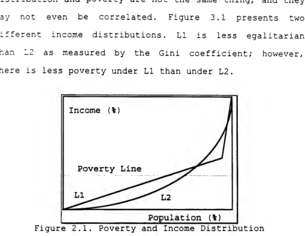
(35) 34. distribution and poverty are not the same thing, ~ay. not. even. di:fe~ent tr,an. be. income as. correlated.. Figure. distributions.. measured. by. the. 11. Gini. 3.1. is. and they. presents. less. two. egalitarian. coefficient;. however,. there is less poverty under 11 than under 12.. Incorne (%). Poverty. Population (%) Figure 2.1. Poverty and Income Distribution. The curves 11 and 12 in Figure 3.1 are called "1orenz curves_''. We measure on the horizontal axis the percentage of the population and on the vertical axis the cumulative income. received. sorted. by. paragraph. their. by. that. income.. illustrate. one. percentage. (from. The. and. of. figure the. problems. O to the. 100%),. preceding. with. income. distribution: i ts measurem~n.t .. ~--- - __ .. -, .. ,...-. The most widely used measure of income inequality is the Gini coefficient:.

(36) G=1-2fL(z)dz. where L(z) Gini. ( 2 .1). is the Lorenz curve. In terms of Fig. 2.1,. coefficient. would. be. twice. the. area. the. between. a. specific Lorenz curve (say 11) and the 45° line. That is, twice the difference between a certain distribution anda perfectly. egalitarian. constructing. this. one.. There. coefficient.. are. First,. two we. problems normally. in have. on_1:_y__5-__or 10 data points, the income received by quintiles or deciles. For sorne cases, like the U.S.A., we might have percentile information, but that happens very seldom. Thearea below the Lorenz curve must then be approximated by rectangles.. The second problem is that L(z). doesn't have. an analytical form. Sorne efforts have been made to find a function Slottje 1991). that and. fits. Johnson,. the. Lorenz. 1990;. curve. Basmann,. (Basmann,. Hayes. and. Hayes, Slottje,. but the main problem is still that the "tails" of. the. distribution are very hard to approximate in a simple .mo.de-1.. Another ~' entropy. which in. measure. of. inequality. is. Theil's. is_ an application of the Shannon comm.u,nJ~ª-ti.91l ___ theory. 1949). TQ~il's index is:. (Shannon. and. entropy index of Weaver,.

(37) 36. ". L(z,). 1=1. .,. H= ¿L(z,)log-. .. ( 2. 2). where, if distribution is completely uniform, all. H=O,. income is in the hands of a single agent,. and if H=ln. n,. where nis the nurnber of agents.. Two. other. income. distribution. indices. are. the. variance..__Qf income defined as ·-·· -- -- ---··. -----·---· -~---·-·- lQgarithms, . ---. ---~-.. .. ~. ... ,-. V=. .. .. nf (togL(z; )-logµ). 2. (2. 3)". 1=1. where V goes from O to infinity as inequality increases. A similar measure is the Coefficient ..of Variation, defined ... __ --- -----·,-, . ~·--_. _.,... ,.. ...,.. '. as. a. CV=µ. ( 2. 4). where a is the standard deviation of income distribution and µ is the mean income..

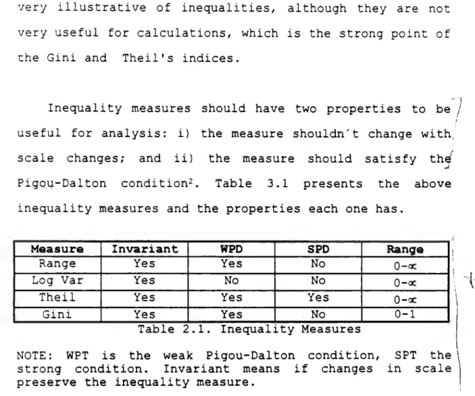
(38) 37. Oth~E' __ E1-e9-Sl.lf~~ earnings. <2_t di._stribution focus on differences in. ( such as Atkinson' s earnings tree). a~on_g - two population subgroups 4 O~). •. or in incorne. (like the top 20% bottorn. The advantage of these me asures. ver y i 11 ustra ti ve o f inequali ties,. is that they are. al though they are not. very useful for calculations, which is the strong point of the Gini and. Theil's indices. - -¡. Inequali ty rneasures should have two properties to be / 1. useful for analysis: i) the rneasure shouldn't change with, scale. changes;. Pigoµ-Dalton. and. ii). the rneasure. condition 2 •. Table. 3.1. should satisfy presents. the. above. inequality rneasures and the properties each one has. Measure. Range Log Var Theil Gini. Invariant. Yes Yes Yes Yes Table 2.1.. WPD. SPD. Yes No No No Yes Yes No Yes Inequality Measures. Ranga O-oc O-oc O-ce 0-1. NOTE: WPT is the weak Pigou-Dal ton condi tion, SPT the 1 strong condition. Invariant means if changes in scale \ preserve the inequality measure. 1. -This condition requires that if a transfer is made from the rich to the poor, the inequality measure must decline. The strong version requires in addition, that if the transfer is made from the rich to a middle-income individual, the measure should differentiate it from the forrner transfer..

(39) 38. Income Distribution and Demographic Factors. One. of. the. developmen~. most. economics. interesting. is. that. relationships. in. demographics. and. between. ir.=ome. If we made a cross sectional study of birth rates and. income. relation. For. per The. example,. Netherlands,. capita,. we. could. easily. see. richer the country,. the. European. (Switzerland,. United. countries. Kingdom,. etc.). fewer. a. have. negative. the births.. an. France,. income. per. capita ranging from 6 to 10 thousand dollars and women in those. countries. during. their. normally. lifetime.. American countries with. an. income. have On. less. the. ( like Mexico,. per. capita. than. other. hand,. Brazil,. below. two. 2,000. children in. Latin. Colombia,. etc.). dollars,. women. normally have between 4 and 6 children in their lifetime (Herrick and Kinjleberger, 1983, p.366).. Furthermore,. the. fewer. people. that. are born. in. the. richer countries tend to live longer. Again from Herrick and Kindleberger(l983, p.365), in very poor countries like Ethiopia, per. capital. years. this. Bangladesh or India people have. In middle goes. up. to. income 60. a. (not more than 200 dollars. life. expectancy of. countries,. years.. Europe. like and. 40. to. 50. Latin Am.erica, other. develope~. countries exhibit life expectancies of 70 to 75 years (all.

(40) 39. data are :hese. from 1980) .. countries. different. from. Nevertheless,. exhibited the. ones. life. lears,. recently as. expectancies. in Asia. years and Norway's around 54,. as. now.. not. Denmark's. very. was. 53. but the rest had about 40. with Russia ~nd Spain very clase to 30 years. Not. surprisingly,. income per capita was also clase to what we. observe today in Asia. Austria had 400 dollars, United Kingdom 900, etc.. In. 1900,. fact,. the. (Dasgupta,. decrease. in. Italy 300,. 388, pp.154-155).. mortality. rates. in. the. underdeveloped countries has been faster than the decline in birth rates,. leading to the demographic boom of this. century (Kuznets, 1983, p.99ff). This indicates that it is possible to live longer without a significant increase in per capi ta. incomes,. thanks to modern surgery and drugs,. but that it is difficult people. towards. to change the behavior of the. reproduction.. The. reason. could. lie. well. beneath the surface. Asan example, peor countries tend to have. more. people. living. in. rural. areas. than. in. ci ties. (Herrick and Kindleberger, 1983, p.389) and in the country more children mean more hands to help in the crops, which seems a good reason not to stop having children 3 •. :isee Gary Becker' s 1993).. analysis. of birth economics. (Becker,.

(41) we. NeverJ:heless,. know. empirically. that. more. a. egalitarian income distribution also means fewer children.. =~. the. fact,. and. distribution. income. between. relation. b i rth rates is stronger than the relation between income The relation between. distribution and income per capi ta.. rural population and income distribution is even stronger (Herrick. Nevertheless, also. normally noted. Kindleberger,. and. in. the. we. not. must. of. case. death. poorer. countries,. population. groups. in. greater. that. forget. 137,366,389).. pp.. 1983,. as in. are. rates. Kuznets U.S.. the. (Kuznets, 1983, pp.101 ff).. The evidence seems to point to what we already noted in. previous. the. chapter:. ~i thout. redist_¡-_ibution growth '- --------- ·. prob~bly is not a very .. de.sir-ab-le objectiYe. Development, or an enhanced quality of life,. seems to be positively. related to both income redistribution and economic growth, at the same time.. The question now should be: Does income distribution d~Ilg__911. 4~qg_;:a_phi~- -~-~~t~_rs also'? That is,. income. between. relationship. two-way. distribution'?. positive. answer.. The. demographic. evidence _,,.. Taub~~!,).__ ___(1974). ------. seems finds. to sorne. is there a and. factors point. to. effects. a on. income distribution by d~mographic factors like education,.

(42) ::n.ent.aL . ªbiJ_i ties .:..:so Kuznets ~ainly. to. (1983,. In. ( like. non-economic. pp.131-239). describe. measurement. factors. and. the. fact,. incentives. addresses this issue,. difficulties. it. seems. associated. that. inGo-m.e. •. but with. mic~Q~demographic religioo.). affect. distribution. affects. e_<:i_l!ca t ioriL ----ªbi li ties,. incorne __ ?,~st_rib~~ton, .while. (pp. 1-2 o). rnacro:-demographic fa-cto:t~f (heal th, poverty, etc.) .. When we. talk. about. income. distribution,. we. tend. to. think that an egalitarian distribution is better than the opposite. This may not be true. As Dasgupta says:. "equality. equal. as. is. everybody. not. so. good.. li ter ate.". Nobody. And. these. (1988,. p.58). litera te two. is. points. as are. obviously different in terms of welfare. Thus egalitarian \ incorne distribution with low incomes might be worse than non-egalitarian distribution of higher incomes, as is the case of the Unites States.. A. very. determine Krueger Wilson. important. most. (1990), (1987). rnicroeconornic __p_r.e_§ent. of. at. Tabellini. point. the. that. inequality.. Perroti. incentives poli tical. and Persson. (1992),. to. ( 1991. f. also. the. (1990), we. rnaintain. level.. institutions. From. Krueger and Orsmond and. the. is. can. papers. lends. of. Findlay and state. inequali ty. Empirical. may. that. rnay. be. evidence. in. support. to. the. /.

(43) 42. point that different institutions may lead to different income distributions.. I!!. Income Distribution and Economic Growth. Since Kuznets's. (1955). study of economic growth and. income distribution and the sequence of "U-curve" articles {for example: Ram, 1991; for a survey on this tapie befare 1990,. see Jung, 1990) , i t has not been possible to reach. an agreement. on. the most. important. question:. income distribution affect economic growth? f ind the answer,. Does. the. In order to. theoretical models .. J1ave been developed. attempting to capture the way that income distribution may et. affect growth. Persson and Tabellini (1991) constructed a model where income distribution affects growth through a pq¡i_tical.. me~h.an_i,_sm. Moulin and Thomson (1988) answer the converse answer. question, is. no,. can. there. growth benefit is. no. everybody?. possibility,. under. Their their. assumptions, that everybody would benefit when the country grows.. A final remark should be that the theoretical efforts have tended to focus only on one aspect ata time, while the question is not whether income distribution affects.

(44) 43. growth. or. relationship grow1:J1?. viceversa,. the. between. income. question. is:. distribution. What and. is. the. economic.

(45) P.ART. II. ECONOMIC GROWTH ANO INCOME DISTRIBUTION. 44.

(46) CHAPTER 3 AN OVERLAPPING GENERATIONS MODEL. In. this. Tabellini. chapter,. that. I. present. analyzes. a. income. model. by. Persson. distribution. and. along. with. economic growth. Most of this chapter is taken from their work,. although I. introduce a modification to their model. that appears in section V.. I. The Model. Persson and Tabellini generations economic model,. model. growth. consumers. consumed. in. the. in. are. which studied. maximize two. ( 1991). income. an overlapping. distribution. simultaneously.. their. periods. present. utility over. they are. allowed. and. In. their. the. goods. to. live.. Utility is defined as. ( 3 .1). where e represents consumption in the first period and d in the second. The superscript i denotes the consumer.. 45. In.

(47) 46. the. f irst. per:iod,. consumption. competes. wi th -~_api tal. accumulation,. 1. c1-1. k. is. the. consumed. capital. during. + k'1 = Y1-1. ( 3. 2). 1. accumulat~J. period. 2,. by. where. i. individual. this. stock. to. of. be. capital. permits period 2 consumption,. ( 3. 3). r. where. is. the. "growth. Redistribution happens which. is. stock,. a. kind. since k,. of is. factor". in this. of. the. country.. second period through 0,. redistributive. tax. on. the. capital. the average stock of capital. in the. country.. Income· in the first period is:. ( 3. 4). where. the term in parentheses is drawn from the. distribution, that. is. dependent. understood here as a stochastic variable e. distributed on. income. capital. with. zero. stock,. k.. mean The. and. a. variance. distribution. is.

(48) 47. generally. specified. distribution exogenously. is. F(e' ,k).. as. assumed. determined. to. be. The. less. endowment. of. median. than. of. one.. "basic. ro. this is. an. abilities". specific to the country.. The program is that at the beginning of period t-1, voters. elect. 91 •. After. that,. investors. select. k1 _ 1 •. A. political-economic equilibrium is defined as a policy and a set of private economic decisions such that: 1) economic decisions are optimal,. for a given redistributive policy,. and markets clear;. The policy can not be defeated by. any. alternative. 2) in. a. majority. election. amongst. the. citizens.. II. Economic Equilibrium. With. homothetic. preferences,. the. intertemporal. decision depends only on prices, that is, on the "interest rate".. Then we can define ; ( =D(r,,9,) 1 ,. D~ <0.. Given this,. we. can. find. the. where. D;>O and. consumed amounts. of. each good,. :r will omit the subindices in the function D far clarity..

(49) 48. (3. 5). and. ( 3. 6). Far the average consumer,. k, = y 1_ 1 -c,_ 1 • We can define the. average rate of growth as g=k,/k,_ 1 -1, that is,. ID 1_ 1D(r ,8) g = -----.-----,.. - 1. (3.7). r, +D(r,8). with g~ > O, g~ < O,. g; > o <. This model is recursive, given an initial condition k and a sequence {8,,ID ,,r,} we can find a growth rate sequence.. III. Political Eguilibrium. Given the utility functional form,. we can rewrite it. like U(c1_ 1 ,d1 )=c,_ 1u(1,D(r,8)), and consequently,. ( 3. 8).

(50) 43. ·.,¡here. +~:~:ir. V(r ,0) = [ 1. U(l,D(r ,0)). ( 3. 9). with >. V8 < O, V, O <. and. W(Cll ,r ,8 ) = oo 1 [ 1+ ( _. 8 1 D(r,8) )( (. 1 8 1 r,+Dr,8. )). ]. ( 3 .1 O). with W¡¡ > O, WCI) = W/oo > O, Weo, = W¡¡/oo > O. Since preferences are linear over e,. they belong to. the class on intermediate preferences studied by Grandmont (1978). Given that v has a unique maximum in 8, we have a median-voter. result:. The. equilibrium. policy. is. the. 8. preferred by the median voter. Let e. be this voter, then the equilibrium policy. 0;. is implicitly defined by. ( 3 .11).

(51) wtich reflects the trade-off that voters face. On the one hand, an increase in 9 redistributes incorne; on the other, it. diminishes. investrnent. and,. therefore,. decreases. the. base for redistribution: general incorne.. IV. Dynarnics of Growth. From the rnodel stated before,. very different growth. patterns can be drawn. Depending on the initial condition of k and the forrn of F(e',k). Sorne of these patterns are non-monotonic, Kuznets'. giving. U curve,. their rnodel,. sorne. theoretical. support. ... or also an inverted U.. for. the. To support. Persson and Tabellini present an empirícal. analysis of different countries with diverse political and economic characteristics. Finally, they pose sorne ways to enrich the model, among them,_ richer savings beh,avior and dis-crimination distribution. about affects. the growth.. mechanism Persson. through and. which. Tabellini. conclude:. l. The main theoretical result is that income inequality is harmful for growth, because it leads · to policies that do not protect property rights and do not allow i full priva te appropriation of returns to investment. (-·-·-(Persson and Tabellini, 1991, p.30) ....

(52) -,. :J.:.. a~d state. that. historical. conclusion. arises. from. evidence. the. fact. supports. that. if. an. this.. This. individual. sa-V~.. in period t-1 in .arder to have more consumption in ~--and t.he rest of the . ªg~nts don' t. save,.. tti.e poli ti cal. equilibriurn will tend to impose a tax on the_ .sªyin_gs _ of the. agent. that. Following this accumulate. saved, argument,. capital. redistributive. making. tax. savings. there. than. are. in. doesn't. fewer. the. exist,. inequality. because. of. is. this. harmful indirect. far. since it. growth. effect. attractive.. incentives. case. and. s ta ted in terms o f the capital stock, Thus,. less. when. to the. growth. is. will be lower. in. this. through. model. poli ti cal. equilibrium and the reduction of incentives to accumulate capital.. V. Minimal. Consumption. Following one of the lines of research proposed by the au thcrs,. I. cons ider a d-i f--fer1;nt ...s.avJpg bE=hªYi.or . in ___ ,the. model through the constraint o.f. a m:il'.l_imal..-eonsump.ti_on. If there. is not enough income for. redistribution. must. have. individuals to survive,. different. patterns.. We. are. assuming that there is a minimal consumption requirement.

(53) S2. denoted by. Crrun.. This. can be. thought. of. as. the. minimal. consumption of goods that allows the country not to suffer a revolt.. Under this restriction,. far certain levels of k 1_ 1 the. country doesn't have political feasibility,. since given a. certain distribution,. be. the. income. will. not. enough. to. consume in period one, leaving savings aside. This doesn't have anything to do with redistributive policy,. since we. are talking about consumption in period one. Nevertheless, when. we. are. not. in. this. extreme. case,. redistributive. policies will have a flocr.. Let us take this case: When income in the first period is enough to consume and save, then it is possible to have a second period, but we are not sure that savings from the. Crrun will be. f irst period will be enough to. ensure that. attained by all. second period.. this. argument,. agents we. find. in. the. the. minimal. 9. that. Following guarantees. political stability:. (3.12). and, solving for. emin.

(54) 53. ( 3 .13). where. ef- is the ability endowment of the individuals that 1. are below the poverty line. Differentiating (/13) against. ~. k1_ 1 we have. (3.14). which is non-positive. These two equations are represented_ graphically. in. Figure. 3 .1,. where. we. can. see. redistributive floor mentioned befare.. Bmm. _c_min_·- - = k . mm (1) +e' 1 -1. k. 1 -1. r -1. Figure 3.1. Minimal Consumption and Capital Restriction. the.

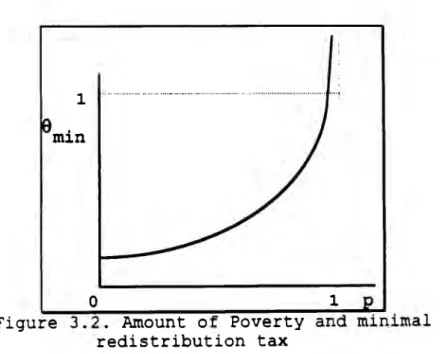
(55) 54. The conclusions are quite interesting, 1s below. (or. to. the. left of). the. if the country. solid line. in 3.1,. pclitical struggle can be predicted. Nevertheless, be better understood if we. look at. it. a. it can. from the poverty. fraction of the country. We have defined a poverty line, and if too many citizens are below it,. enun. grows up. to. 100 %. Differentiate (3.13) against p to find. ( 3 .15). which tends asymptotically to infinity as p tends to one. Figure 3.2 presents this case.. 1. ···················· ····················· ............. ............. min. O 1 Figure 3.2. Amount of Poverty and minimal redistribution tax.

(56) 55. Now,. what. happens. with. growth?. As. in. the_ origi~l. rnodel, the greate~ the need for redistribution, the slower ··-- ----. ·- ..._______ . ~l"l-~_r'3:__~e_o_t_grg_w~_h. Then, from 3.15 the greater the amount o f QQ9_r pE:!g_E_!~l ... the s-lower -.:.ha country --wi 11 grow. I f the re 1s a poverty trap 1 anywhere, this is it.. Under this modification to the model of Persson and Tabellini,. their. conclusions. become. stronger.. If. inequality was harmful for-._growth in the _Qtlgina.J...-m.odel, because of poli tical equi-1-i-brium, under t-a-e--n-ew--ass.um~tion inequality might even-le·ad·--to···p-olitic-al·-un-f-easibility -tor ~. country.. period,. Far certain levels of capital in the starting. the country doesn' t. redistributi ve. efforts.. may actually be. even have a chance to apply. At. first. suffering this. glance, disease.. sorne Note. countries that. this. result depends on the assumptions on the voting capability of poor people. If they are not allowed to vote, then the minimal fact,. redistributive. tax would be. Persson and Tabellini. restricted. to. the. rich. also. people,. faster since no redistributive tax big). very different.. find the. that. country. if. In. vote. will. is. grow. (or at least not very. will be imposed on the capital stock, -avoiding the. reduction argument. of. incentives. still holds. to. save.. Nevertheless,. our. since even if peor people are not.

(57) 56. allowed to vote,. Lf the redt~tributive. tax is not enough. to permit everyone fulfill basic needs. (that is what Cmm. 1s. about). then the political. feasibility of the country. becomes endangered since the cost of continuing under the political. system becomes excessive far. the peor and the. cost of joining a revolt becomes relatively smaller. !his a¡:gi¿m_ent may exJ:;>lain -the.-successive political reforms. in. ··--··· - - - - - - - - · - - · · - · - ---¡. underdeveloped countries rich people,. tha.t. are. normally condemn-ed.-,,by. since those reforms lead to tax and subsidy. increments while. the. government defends. them by stating. that the stability of the country is more important than economic growth in those circumstances. Also this argument may. be. effective. in. dealing. with. the. issue. that. sorne. countries do not reach political stability if not ruled by. .. ,. dictators, being at the same time very poor countries. The. poor-unstable duality that, for example, Latin American or African countries suffermay be, in fact, a vi-ei-ous circle resting. on. a. faulty. redistributive efforts.. combina.tion. of. capit-al - s ~. and.

(58) CHAPTER 4 APPROXIMATING THE LORENZ Ct:RVE. Approximating the Lorenz curve has been a major issue in. empirical. (1897), finding. work. on. income. distribution.. Pareto. a considerable amount of effort has been spent in a. function. that. approximates. example, Aitchinson and Brown, In particular Basmann, and Basma~n, that. Since. Hayes,. the. curve. (for. 1957; Champernowne,. 1953).. Slottje and Johnson. (1990). Hayes and Slottje. approximates. this. (1991). Lorenz. curve. presenta function which. can. also. be. interpreted in terms of the difficulty of moving up the income distribution.. In this chapter a different function. is presented that makes a somewhat better approximation to the curve.. I. The Function. An· interesting approach to the Lorenz curve is the use of. the. mobility function.. Basmann. et. al.. (1990,. 1991). define the mobility function as the perceived difficulty of moving up in the income distribution. difficulty. is. assumed. to. be 57. a. function. This perceived of. the. agent' s.

(59) current position. The steeper the Lorenz curve around the actual position of the agent, the greater the difficulty . 7~e Lorenz curve is. L(z) = Azª (y -. where. a>l,. function of. and y>l.. '3<0. zl. ( 4. 1). really. parameter A is. The. a. and '3, since 1(1) must be l. Then. y. A= (y - 1rll. ( 4. 2). L(z) = z11 ( Y - z)ll y -1. ( 4. 3) .. substituting, we have. dependent only on three parameters. This function will be called the. hereafter). _9.amma function". 11. (which. has. the. following derivative with respect to z:. cL(z). oz. I (z). is. =/(r.) = L(z>[ª __'3_] z. ( 4. 4). z. function. -,It can-- .b.e -percei ved difficulty fór incfividuals to. as. defined. y -. the. mobility. -- --···----------·--··--··-----.. understood as the move .. . up. Jn. rnonotonically. the. distribution.. increasing,. meaning. This that. the. function. is. closer. one.

(60) 59. individual. is to. the top of the distribution,. the more. d~:ficult it will be to move further up. Note that in the case. of. a. completely. egalitarian. distribution,. this. ~otility function would be a constant, that is to say, if --e.,1-e:i:;-y-body has the same earnings, there is no difficulty inchanging. position.. As. z. approaches. zero,. L(z). also. approaches zero, making I(z) a very small quantity. When z approaches. 1,. L(z). does. the. same. and. I(z). approaches. infinity.. The interesting theoretical properties come from the intuition. behind. the. parameters.. is. a. the. major. determinant of the shape of the lower portian of z (as z~ O), while. P. and y are more influential in the upper part. of the curve,. that is, when z~l. The derivative of L(z). with respect to a is. ol(z). - - = L(z)ln(z) ~ O. (4. 5). aa. which means that an increase in a will reduce the income received by all the agents since but. with. middle. a. part. greater of. impact. the. (in. (4.5). is non-positive,. absolute. distribution.. terms). on. Nevertheless,. the the. relative effect of a change in a will be more important in.

(61) the lower part of the curve, declining around z>0.3. y. J3. and. are the majar determinants of the upper portian of the. d:s:ribution. The derivatives with respect to J3 and y are. e~(:). cJ3. =L(z)ln(y-:)~o y- l. cL__(z) = ay. which. are. always. L(z)(-J3-)( z- l) ~ O y-z y-1. non-negative. increasing. An increase in. ( 4. 6). and. P (J3~0, since. (4. 7). monotonically J3 is always less. than or equal to O) will increase the income received by all agents except for z=l, becomes. more. egalitarian.. that is, In. fact,. income distribution when. a=l. and. J3=0,. income distribution is uniform. An increase in y produces the. same. result:. A. more. egalitarian. distribution. of. income.. II. Empirical Results. The challenge. function for. L(z). is. non-linear.. A very important. empirical analysis of income distribution. data is that we normally have only five, or at most ten, data points to estimate the function. It is very difficult.

(62) r,. e-. to. have. initialization. ,nea.::ingful non-linear data. points.. f·...::-.c:ion. is. good. enough. regression resul ts. interesting. An. L(z). values. that. empirical. using y=l. and. to. get. using only ten property. then. of. the. estimating a. li~earized version of L(z), gives us these initialization ,,alues.. We. can. apply an. iterative method. using. linear. regressions to obtain the non-linear parameters, using an algorithm like l. Set y=l.. 2 . Run linear regression to estimate In L(z) = In A + a ln z + PIn( y - z) • 3. Set y"=. 4.. If. exp(,½tn(½))+ l. lrv-Y i>e. then. y=y",. go. to. 2,. else. finish.. This ~lgorithm makes use of the fact that L(l)=l. At this point, if we solve for y, we obtain the equation used in. step. 3.. Introducing. the. new. value. of. y. into. the. function in step 2 leads us to another value of A. Since the derivative of behaved. function,. L(z). against y. also. (eq.. 4.7). monotonically. is. a well-. increasing,. convergence is rapid, and it is generally useful to start with a low value of y, like l..

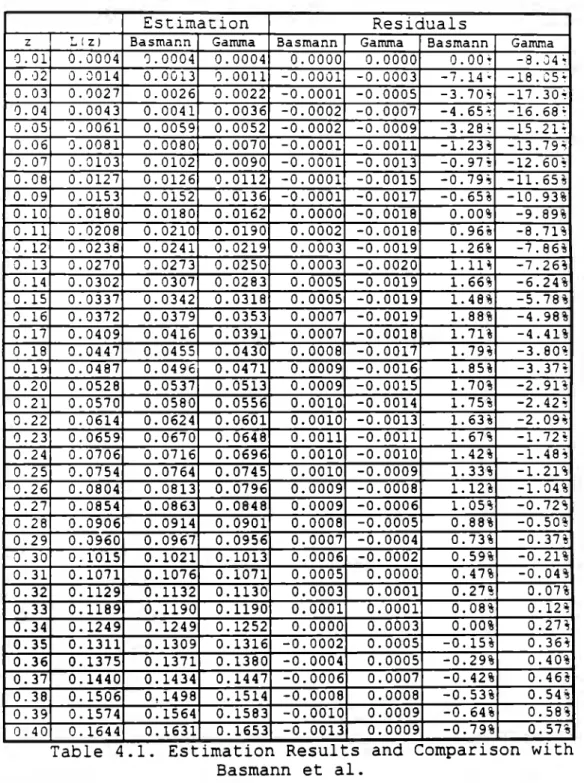
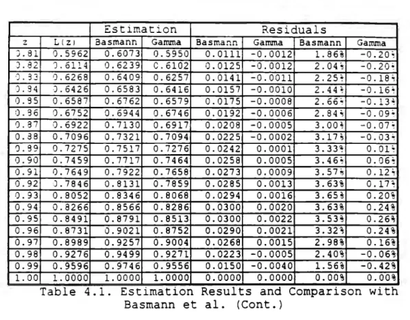
(63) '? 2. In fact,. P are very stable parameters. Linear. a. and. regressions for a sample of thirty countries find that a. :..s. normally. :nterval. between. 1.5. and. 1.8,. while. p lies in the. [-0.1,-0.2]. Using these initialization values,. we obtain very good non-linear regression resul ts. not clear what r. 7ber of data points. is. It is. the mínimum to. obtain good results in the regression, but ten points have worked well.. Using this data. gives. function to estímate income distribution. us. results. that. obtained. by. Basmann. et. presents. the. resul ts. using. al.. are. comparable. to. 1991).. Figure. 4.1. function wi th. the. (1990,. the. gamma. those. data provided by Basmann et al. along with the results of Basmann and the actual values of the Lorenz curve using U.S.. income distribution data far 1977. As can be clearly. seen, the estimated gamma function lies closer to the real values.. Figs. 4.2,. of. distribution. the. regions.. It. is. 4.3 and 4.4 present different sections in. evident. arder. to. identify. that. the. gamma. better than the model of Basmann et al.. the. function except. lowest portian of. the distribution. In fact,. and. the. 4.6. present. residuals. of. both. critical works. for. the. figures. 4.5. functions.. In. absolute terms,. the gamma function is always better than. the. al.. Basmann. et. function.. Nevertheless,. in. relati ve.

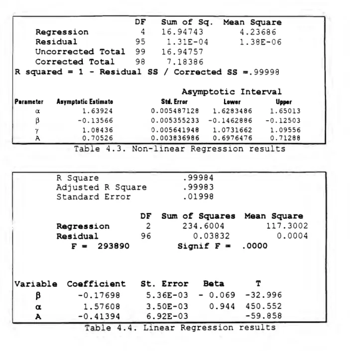
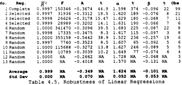
(64) te~~s,. the gamma function is worse in the first quintile,. a~d better from there on.. Table 4.1 presents the results for these one hundred da~a points. The first two columns contain both estimates, the middle columns present the absolute residuals, and the last. two. presents. columns the. sum. the of. relative. squares. residuals.. for. both. Table. estimations,. 4.2 in. absolute and relative terms. The gamma function is clearly better in absolute terms,. but the residuals in the first. decile make it worse in relative terms.. This. big. difference. in. the. case. of. the. relative. residuals may be related to the numerical procedures. fact,. In. using the algorithm presented above, parameters are. somewhat different. Table 4.2 also presents these results. Not surprisingly, absolute errors are bigger in the linear regressions. but. relative. errors. are. smaller.. Fig.. 4.7. presents a graphical comparison of the two procedures for estimating. gamma,. Basmann et al.. along. model.. with. the. estimates. Table 4. 3 presents. regression resul ts while Table. using. the. the non-linear. 4. 4 presents. the. (final). linear estimation results. An interesting additional point for. the. linear. estimation. is. that. the. iterative. linear.

(65) é4. :echnique allows. successfully estímate. to. us. Lorenz. the. cur7e using only five data points.. A final point could be rnade here. Estirnations seem to be very consistent. Several tests were performed with the data. table. in. shown. observations. and. 4 .1. selecting. estimating. randomly. parameters.. the. 6. 4,. or. Results. 8 of. these tests are in table 4.5 and we can see that standard deviations of the parameters are quite small. Maybe the parameter that suffers most from small samples is. p.. III. Cross-Country ar.d Time-Series. Using. data. from. World. the. Bank. (1984),. we. have. estimated the gamma function pararneters for 28 countries. The data appear 4.7.. in table. and the resul ts. 4. 6,. in table. This exercise gives usa good idea of the values of. the parameters for a wide range of different cultures and institutions.. This. will. be. of. great. help. in. the. next. chapters.. A time-series exercise was also made using data from Mexico. (IMSS-COPLAMAR,. 1981;. INEGI,. 1988;. INEGI,. 1992),. presented in table 4.8. The results (Table 4.9) seem quit~.

(66) 65. consistent with the cross-country case. They will also be ~sed in the next chapter.. Estimation z 'J.01 O. •)2 0.03 0.04. o.os 0.06 0.07 0.08 0.09 0.10 O.11 0.12 0.13 0.14 0.15 0.16 0.17 0.18 0.19 0.20 0.21 0.22 Q. 2 3 0.24 0.25 0.26 0.27 0.28 0.29 0.30 0.31 0.32 0.33 0.34 0.35 0.36 0.37 0.38 0.39 0.40. I.. 1 z l. 0.0004 O.:J014 0.0027 0.0043 0.0061 0.0081 0.0103 0.0127 0.0153 0.0180 0.0208 0.0238 0.0270 0.0302 0.0337 0.0372 0.0409 0.0447 0.0487 0.0528 0.0570 0.0614 0.0659 0.0706 0.0754 0.0804 0.0854 0.0906 0.0960 0.1015 0.1071 O.1129 O.1189 0.1249 0.1311 0.1375 O .1440 0.1506 0.1574 0.1644. Basmann 'J.0004 0.0013 0.0026 0.0041 0.0059 0.0080 0.0102 0.0126 0.0152 0.0180 0.0210 0.0241 0.0273 0.0307 0.0342 0.0379 0.0416 0.0455 0.0496 0.0537 0.0580 0.0624 0.0670 O. 0716 0.0764 O. 0813 0.0863 O. 0914 0.0967 0.1021 0.1076 O. 1132 0.1190 0.1249 0.1309 0.1371 O .1434 0,1498 0.1564 0.1631. Gamma 0.0004 O. 0011 0.0022 0.0036 0.0052 0.0070 0.0090 O. 0112 O. 0136 0.0162 0.0190 0.0219 0.0250 0.0283 0.0318 0.0353 0.0391 0.0430 0.0471 0.0513 0.0556 0.0601 0.0648 0.0696 0.0745 0.0796 0.0848 0.0901 0.0956 O. 1013 O.1071 O.1130 O.1190 0.1252 0.1316 o. 1380 0.1447 O.1514 0.1583 0.1653. Residuals Basmann 0.0000 -0.0001 -0.0001 -0.0002 -0.0002 -0.0001 -0.0001 -0.0001 -0.0001 0.0000 0.0002 0.0003 0.0003 0.0005 0.0005 0.0007 0.0007 0.0008 0.0009 0.0009 0.0010 0.0010 O. 0011 0.0010 0.0010 0.0009 0.0009 0.0008 0.0007 0.0006 0.0005 0.0003 0.0001 0.0000 -0.0002 -0.0004 -0.0006 -0.0008 -0.0010 -0.0013. Gamma Basmann 0.0000 O. 00 + -7.14~ -0.0003 -0.0005 -3.70".5 -0.0007 -4. 65". -0.0009 -3.28~ -o. 0011 -1.23, -o. 0013 -0.97! -0.79".S -0.0015 -0.0017 -0.65% -0.0018 0.00% -0.0018 O. 9611 -0.0019 1.26% -0.0020 1.1111 -0.0019 1.66% -0.0019 1.48% -0.0019 l. 88% 1.71% -0.0018 l. 79% -0.0017 l. 85% -0.0016 -0.0015 1.70% -o. 0014 1.75% -0.0013. l. 63% -o. 0011 1.67% l. 42% -0.0010 -0.0009 1.33% 1.12% -0.0008 -0.0006 1.05% -0.0005 0.88% 0.73% -0.0004 0.59% -0.0002 O. 47% 0.0000 0.27% 0.0001 0.08% 0.0001 0.00% 0.0003 -0.15% 0.0005 -0.29% 0.0005 -0.42% 0.0007 -0.53% 0.0008 -0.64% 0.0009 -0.79% 0.0009. Gamma -8.J4• -18.CS-: -17.30". -16.68~ -15.21~ -13.79~ -12.60~ -11. 65% -10.93% -9.89% -8. 71% -7.86% -7.26% -6.24% -5.78% -4.98% -4. 41%. -3.80~ -3.37! -2.9H -2.42~ -2.09% -1.72~ -1.48's -1.21% -1. 04% -o. 72% -0.50% -0.37% -o. 21% -0.04% 0.07% 0.12% 0.27<s O. 36% 0.40% 0.46% O. 54".5 0.58% o. 57%. Table 4.1. Estimation Results and Comparison with Basmann et al..

(67) Estirnation z O.H J.42 :, . 4 3 O. 4 4 0.45 0.46 0.47 0.48 0.49 o.so 0.51 0.52 0.53 0.54 O.SS 0.56 0.57 0.58 0.59 0.60 0.61 0.62 0.63 0.64 0.65 0.66 0.67 0.68 0.69 0.70 0.71 0.72 0.73 0.74 0.75 0.76 0.77 0.78 0.79 0.80. L (zl. O. 1716 ,J. 178 8 'J. l8 62 '.J .1937 0.2014 0.2093 0.2:.73 0.2255 0.2339 0.2424 0.2511 0.2599 0.2689 0.2780 0.2873 0.2968 0.3064 0.3162 0.3262 0.3364 0.3467 O. 3572 0.3679 0.3787 0.3898 0.4010 0.4125 0.4241 0.4360 0.4481 0.º4603 0.4728 0.4655 0.4984 O. 5116 0.5250 0.5387 0.5526 0.5669 0.5814. Basmann 0.1699 'J. 1769 0.1841 0.1914 0.1988 0.2064 0.2142 0.2221 0.2302 0.2385 0.2470 0.2556 0.2644 0.2734 0.2826 0.2920 0.3016 O. 3114 0.3215 0.3317 0.3421 0.3528 0.3637 0.3749 0.3863 0.3979 0.4098 0.4220 0.4344 0.4471 0.4601 0.4734 0.4870 0.5009 0.5151 0.5296 0.5444 0.5596 0.5751 0.5910. Res1duals. Gamma. Basmann. Gamma. 0.1725 '.J .1798 0.1873 0.1949 0.2026 0.2105 0.2185 0.2267 0.2350 0.2435 0.2521 0.2609 0.2699 0.2789 0.2882 0.2976 O. 3071 0.3169 0.3268 0.3368 O. 34 71 0.3575 0.3680 0.3788 0.3898 0.4009 0.4122 0.4238 0.4355 0.4475 0.4596 O. 4 720 0.4846 0.4975 0.5106 0.5240 0.5376 0.5515 0.5657 0.5802. -o. 0017 -0.0019 -0.0021 -0.ü023 -0.0026 -0.0029 -0.0031 -0.0034 -0.0037 -0.0039 -0.0041 -0.0043 -0.0045 -0.0046 -0.0047 -0.0048 -0.0048 -0.0048 -0.0047 -0.0047 -0.0046 -0.0044 -0.0042 -0.0038 -0.0035 -0.0031 -0.0027 -0.0021 -0.0016 -0.0010 -0.0002 0.0006 0.0015 0.0025 0.0035 0.0046 0.0057 0.0070 0.0082 0.0096. 0.0009 0.0010 0.0011 0.0012 0.0012 0.0012 0.0012 0.0012 0.0011 0.0011 0.0010 0.0010 0.0010 0.0009 0.0009 0.0008 0.0007 0.0007 0.0006 0.0004 0.0004 0.0003 0.0001 0.0001 0.0000 -0.0001 -0.0003 -0.0003 -0.0005 -0.0006 -0.0007 -0.0008 -0.0009 -0.0009 -0.0010 -0.0010 -o. 0011 -o. 0011 -0.0012 -0.0012. Basmann -o. 99-; -1. 06~ -1.13~ -1.19~ -1.29~ -1.39~ -1. 43~ -1.SU -1. 58% -1. 61~ -1.63~ -1. 65% -1. 67'1 -1.65% -1. 64% -1. 62, -1.5n -1.52, -1.40 -1.40% -1. 33% -1.23% -1. 14% -1. 00% -0.90% -o. 77% -0.65% -O.SO% -0.37% -0.22% -0.04% 0.13% 0.31% O. 50'.<i 0.68% 0.88% 1.06% 1.27% 1.45% l. 65%. Garnrr.a 0.53~ o.se~ 0.58~ 0.61~ 0.6i~ 0.58~ O. 57 • 0.54~ 0.49~ O. 46-! 0.42'! 0.39~ 0.35, 0.34% 0.31% 0.26% 0.24% 0.21% 0.17% 0.12% 0.10%. o.on 0.04~ O. 03• -0.01~ -0.02% -0.06% -o. 08'.<i -0. lH -0.14% -0.14% -0.16% -0.18% -0.18% -0.19% -0.20% -0.20"5 -0.20% -0.21% -0.21%. Table 4.1. Estirnation Results and Cornparison with Basrnann et al. (Cont.}.

(68) 67. Estimation z. LIZI. J.81 J.82. 0.5962 'J. óll4 iJ.6268 J.ó426 0.6587 0.6752 0.6922 0.7096 0.7275 0.7459 0.7649 ).7846 0.8052 0.8266 0.8491 0.8731 0.8989 0.9276 0.9596 1.0000. ·J. 3 3 J.34 0.95 :) . 3 ó 0.87 0.38 'J. 99 0.90 0.91 0.92 :J. 9 3 0.94 0.95 0.96 0.97 0.98 0.99 l. 00. aasmann 0.6073 0.6239 0.6409 0.6583 0.6762 O.ó944 0.7130 0.7321 0.7517 O. 7717 0.7922 0.8131 0.8346 0.8566 0.8791 0.9021 0.9257 0.9499 0.9746 1.0000. Residuals. Gamma Basmann Gamma Basmann 0.5950 O. 0111 -0.0012 l. 86% C.ól02 2. 04, 0.0125 -0.0012 0.6257 0.0141 -o. 0011 2.25• 0.0157 -0.0010 0.6416 2.44~ 0.6579 2. 6ó;, 0.0175 -0.0008 0.6746 0.0192 -0.0006 2. 84 'l 3.00, 0.6917 0.0208 -0.0005 3 .17, 0.7094 0.0225 -0.0002 O. 7276 0.0242 0.0001 3.33~ 0.7464 0.0258 0.0005 3.46~ 0.7658 3.57~ 0.0273 0.0009 0.7859 0.0285 0.0013 3.63% 0.8068 0.0294 0.0016 3.65% 0.8286 3.63% 0.0300 0.0020 0.8513 0.0300 0.0022 3.53% 3.32, 0.8752 0.0290 0.0021 0.0268 2.98% 0.9004 0.0015 O. 9271 0.0223 -0.0005 2.40% 0.9556 0.0150 -0.0040 l. 56% 0.00% 0.0000 l. 0000 0.0000. Gamma -0.20'5 -0.20• -0.18· -0.16« -0.13~ -0.09• -0.07~ -0.03-: 0.01• O. 06• 0.12~ 0.17• 0.20% 0.24% 0.26~ 0.24% 0.16% -0.06% -0.42% 0.00%. Table 4.1. Estimation Results and Comparison with Basmann et al. (Cont.). Gamma Linear Non-Linear 0.000948 0.000131 0.01079 0.040764 0.226815 0.03723 Table 4. 2. Sum of Squared Residuals Basmann. Absoluta Relative.