TítuloFundamentals of TGA and SDT

Texto completo

(1)Fundamentals of TGA and SDT Weibing Xu, Sen Li, Nathan Whitely and Wei-Ping Pan Thermal Analysis Laboratory, Materials Characterization Center, Western Kentucky University, Bowling Green, KY 42101 [email protected] Thermal analysis is one of the most useful methods of analysis in collecting both physical and chemical information. Probably the most used technique of thermal analysis is thermogravimetric analysis (TGA). TGA is used in all types of applications, providing information about the bonding of components within the sample. TGA can become an even stronger analytical technique when coupled with other thermal analysis techniques such as differential scanning calorimetry (DSC) and spectroscopic techniques such as Fourier transform infrared spectroscopy (FTIR) and mass spectrometry (MS). TGA measures the absolute amount and rate of change in weight of a sample as either functions of time or temperature in a controlled environment. TGA has a wide range of properties that can be measured such as thermal stability, oxidative stability, effects of different atmospheres, moisture and volatile content, and sometimes the composition of multi-component systems. TGA determines if and how different components within a material are bonded differently. When TGA is coupled with DSC or differential thermal analysis (DTA), the mode of analysis is called simultaneous DSC-TGA (or DTA) (SDT). SDT measures the amount and rate of change in weight, but also measures the heat flow of the sample as a conventional DSC does. SDT measures the same properties as TGA, but extends the list to include heats of reactions, melts, and boiling points. The three most important signals that TGA collects while it is analyzing the sample are weight, rate of weight change—differential thermogravimetry, and temperature. A differential thermogravimetry curve—DTG—is generated as the first derivative of the weight with respect to temperature or time. The DTG curve can be used to provide both qualitative and quantitative information about the sample. Qualitative modes of analysis include fingerprinting a material and distinguishing between two or more overlapping reactions. Quantitative modes include peak height and temperature at maximum weight loss measurements. The most important aspect of TGA operation is the validity of measurements made. Confidence in data collection can be achieved through regular calibration. For TGA, both mass and temperature calibrations must be performed. Most instrument and software packages possess a relatively automated mass calibration procedure in which the user places certified calibration weight onto the instruments sample platform. Temperature calibrations are performed by the calculation of the Curie point of standard metals. The Curie point of a material is the temperature at which the material loses its magnetic susceptibilities. To perform the Curie point temperature calibration, a strong magnet must be place below or on top of the furnace the cause an initial weight gain or loss at room temperature. Figures 1and 2 show the experimental apparatus for both vertical and horizontal instrumental configurations..

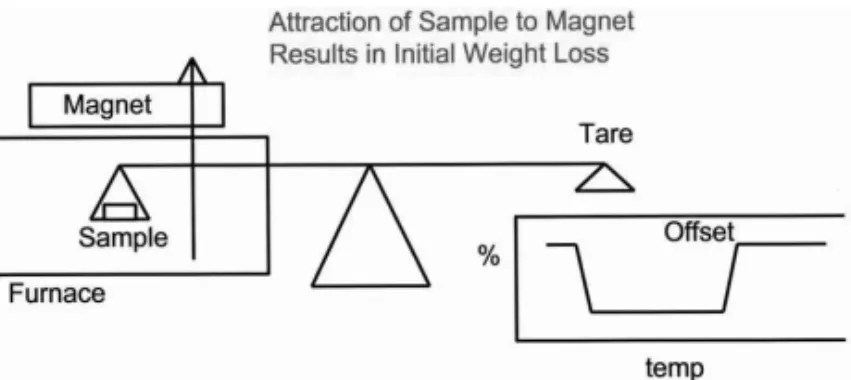
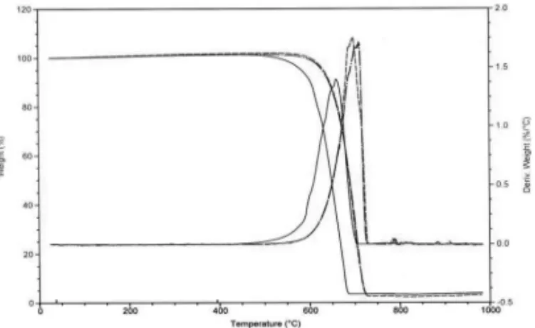
(2) 2. WEIBING XU, SEN LI, NATHAN WHITELY AND WEI-PING PAN. Figure 1. Horizontal temperature calibration configuration. Figure 2. Vertical temperature calibration configuration A small lab jack can be used to adjust the magnet’s distance from the sample such that a 2-3% weight gain or weight loss occurs once the magnet is positions above or below the sample. Figure 3 shows the Curie point determination for nickel and alumel. Note that the Curie point is denoted as the offset.. Figure 3. Curie point determination for vertical TGA SDT also has an alternate method for temperature calibration. The melting points of standard materials can be determined by the onset of the endotherms and compared to the theoretical melt temperature. A good exercise for both TGA and SDT is to perform multiple analyses of calcium oxalate monohydrate. By performing such.

(3) FUNDAMENTALS OF TGA AND SDT. 3. an analysis the performance and precision of both you and the instrument can be measured. An overlay of five calcium oxalate experiments is shown in Figure 4.. Figure 4. Performance testing using calcium oxalate monohydrate Although calcium oxalate monohydrate is not typically a standard material, it does hold good utility in intra-laboratory analysis. The weight change and peak temperature can be inputted into a spreadsheet program to check your instrument and operators performance. The accuracy of the instrument can be used to assess your instruments long-time performance, and help single out a damaged component of the instrument. The baseline can also be quite usual in quantifying your instrument’s performance and sensitivity. Small weight losses become increasingly difficult to measure if the instrument’s baseline is large compared to that of the instrument. TGA is the foremost analysis technique in determining quantitative properties of the original sample. A polyethylene (PE) sample filled with CaCO3 was analyzed as shown in Figure 5.. Figure 5. TGA curve of polyethylene sample filled with calcium carbonate By knowing the degradation reaction of CaCO3, the initial percentage of CaCO3 in the PE can be calculated. At approximately 550ºC the PE is completely decomposed; thus, the weight loss occurring at approximately 650ºC is due to the decomposition of CaCO3. The weight loss is a direct result of the evolution of CO2 gas. The residue is the remaining CaO that fails to decompose. From the weight change and the residue,.

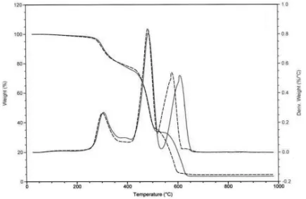
(4) 4. WEIBING XU, SEN LI, NATHAN WHITELY AND WEI-PING PAN. the stoichiometric relationships can be used to determine a percentage of CaCO3 that exists in the original PE sample. Calculating the initial percentage of CaCO3 from the weight change is more accurate than calculating it from the residue. Most polymers contain fillers; hence, the residue is a combination of CaO and these fillers making this calculation less accurate. TGA and SDT can also be used to demonstrate the important of reaction atmosphere. Calcium oxalate monohydrate was analyzed under the same experimental conditions except the purge gas. The sample was analyzed in air, CO2, and nitrogen of equal flow rates. Figure 6 illustrates Le Chatilier’s principle.. Figure 6. Le Chatilier’s principle shown using TGA Because the degradation of CaC2O4 produces CO2, the reaction is inhibited when it occurs in a CO2-saturated atmosphere. Figure 7 shows the heatflow data collected with the SDT.. Figure 7. DSC Curve of calcium oxalate monohydrate in multiple atmospheres The CaC2O4 oxidizes in air as shown by the endotherm at approximately 500ºC while in nitrogen and CO2 oxidation does not occur but rather pyrolysis. Hi-Resolution TGA is useful to separate overlapping weight losses. HiResolution TGA exposes the sample to an isotherm once a weight loss is detected. The isotherm allows the weight loss occurring at the lower temperature to complete before the second weight loss begins. Figure 8 shows that as the resolution increases, the two weight losses are more separate and defined..

(5) FUNDAMENTALS OF TGA AND SDT. 5. Figure 8. TGA curves at multiple hi-resolution settings Quality control testing often exposes a product to a particular atmosphere for very extended periods of time which can be costly and time consuming. TGA in conjunction with kinetics software can be used to decrease the time and money spent on tedious lifetime testing procedures. A sample is analyzed over the same temperature range using at least four different heating rates. Software is then used to generate numerous plots that can predict the product’s performance over time. The activation energy, rate constant, and other kinetics related information can be provided as seen in Figure 9.. Figure 9. Log[heating rate] curve at multiple conversions Figure 10 shows the lifetime of the sample at varying isotherms..

(6) 6. WEIBING XU, SEN LI, NATHAN WHITELY AND WEI-PING PAN. Figure 10. Lifetime plot for polymer sample Although this lifetime plot may not eliminate the need for lengthy quality control testing, it may help predict poorly performing products at an earlier stage in the production process. Two automotive belts composed of alkylated chlorosulfonated polyethylene (ACSM) were tested using TGA to identify the reason why one belt performed at 10% of a normal functioning belt. The belts were analyzed under the exact heating rates under an air atmosphere. The belts each showed the typical degradations profile of a rubber sample as seen in Figure 11.. Figure 11. TG and DTG Curve of Passed and Failed Belt Sample in Air Oil was decomposed first followed by the decomposition of the polymer, and finally the carbon black combusted with the oxygen in the air. This analysis showed that both the oil and polymer portions of the rubber were not the cause of the bad belt’s failure. The decomposition of the bad belt was approximately 20ºC lower than the good belt. Figure 12 shows that the bad belt was composed of carbon black 1, which has the lower decomposition temperature..

(7) FUNDAMENTALS OF TGA AND SDT. 7. Figure 12. TG and DTG Curves of Carbon Black Components of Failed Belt Sample TGA and SDT can used be in nearly any application to gather information. TGA and SDT provide a method of analysis that is fast and easy to operate, but provides precise and accurate results. In situations where TGA and SDT cannot be used to study a system directly, TGA and SDT can provide estimations that help alleviate some of the difficulty in using more complicated analysis methods.. Acknowledgements Many thanks to Len Thomas of TA Instruments who allowed use of his short course presentation given at Western Kentucky University..

(8)