HATS 36b and 24 Other Transiting/Eclipsing Systems from the HATSouth K2 Campaign 7 Program

Texto completo

(1)The Astronomical Journal, 155:119 (14pp), 2018 March. https://doi.org/10.3847/1538-3881/aaa8e6. © 2018. The American Astronomical Society. All rights reserved.. HATS-36b and 24 Other Transiting/Eclipsing Systems from the HATSouth-K2 Campaign 7 Program D. Bayliss1,2 , J. D. Hartman3 , G. Zhou4 , G. Á. Bakos3 , A. Vanderburg4 , J. Bento5, L. Mancini6,7,8, S. Ciceri7, R. Brahm9,10 , A. Jordán9,10 , N. Espinoza9,10 , M. Rabus7,10 , T. G. Tan11 , K. Penev3 , W. Bhatti3 , M. de Val-Borro3 , V. Suc10 , Z. Csubry3, Th. Henning7, P. Sarkis7, J. Lázár12, I. Papp12, and P. Sári12 1. Observatoire Astronomique de l’Université de Genève, 51 ch. des Maillettes, 1290 Versoix, Switzerland; [email protected] 2 Dept. of Physics, University of Warwick, Gibbet Hill Road, Coventry CV4 7AL, UK 3 Department of Astrophysical Sciences, Princeton University, NJ 08544, USA 4 Harvard-Smithsonian Center for Astrophysics, 60 Garden Street, Cambridge, MA 02138, USA 5 Research School of Astronomy and Astrophysics, Australian National University, Canberra, ACT 2611, Australia 6 Dipartimento di Fisica, Università di Roma Tor Vergata, Via della Ricerca Scientifica 1, I-00133, Roma, Italy 7 Max Planck Institute for Astronomy, Königstuhl 17, D-69117 Heidelberg, Germany 8 INAF—Osservatorio Astrofisico di Torino, Via Osservatorio 20, I-10025, Pino Torinese, Italy 9 Millennium Institute of Astrophysics, Av. Vicuña Mackenna 4860, 7820436 Macul, Santiago, Chile 10 Instituto de Astrofísica, Facultad de Física, Pontificia Universidad Católica de Chile, Av. Vicuña Mackenna 4860, 7820436 Macul, Santiago, Chile 11 Perth Exoplanet Survey Telescope, Perth, Australia 12 Hungarian Astronomical Association, 1451 Budapest, Hungary Received 2017 June 10; revised 2017 December 14; accepted 2017 December 20; published 2018 February 16. Abstract We report on the result of a campaign to monitor 25 HATSouth candidates using the Kepler space telescope during Campaign 7 of the K2 mission. We discover HATS-36b (EPIC 215969174b, K2-145b), an eccentric (e = 0.105  0.028) hot Jupiter with a mass of 3.216  0.062 MJ and a radius of 1.235  0.043 RJ , which transits a solar-type G0V star (V=14.386) in a 4.1752-day period. We also refine the properties of three previously discovered HATSouth transiting planets (HATS-9b, HATS-11b, and HATS-12b) and search the K2 data for TTVs and additional transiting planets in these systems. In addition, we also report on a further three systems that remain as Jupiter-radius transiting exoplanet candidates. These candidates do not have determined masses, however pass all of our other vetting observations. Finally, we report on the 18 candidates that we are now able to classify as eclipsing binary or blended eclipsing binary systems based on a combination of the HATSouth data, the K2 data, and follow-up ground-based photometry and spectroscopy. These range in periods from 0.7 day to 16.7 days, and down to 1.5 mmag in eclipse depths. Our results show the power of combining ground-based imaging and spectroscopy with higher precision space-based photometry, and serve as an illustration as to what will be possible when combining ground-based observations with TESS data. Key words: planetary systems – stars: individual (HATS-36) – techniques: photometric – techniques: spectroscopic Supporting material: figure set, machine-readable table plane fields since 2014. K2 Campaign 7 (C7) monitored a field centered at a = 19 h 11m 19s, d = -2321¢36 between 2015 October 4 to 2015 December 26. By chance, approximately 25% of this field had already been monitored by the HATSouth survey five years earlier between 2010 March to 2011 August. It was therefore possible for us to propose for K2 targets based on the HATSouth light curves that showed transit-like signals, and this was done as part of the K2 Guest Observer program (GO7067; PI: Bakos). In addition, we were also able to select as K2 targets the HATSouth transiting planets that had already been confirmed as bona fide planets, namely HATS-9b (Brahm et al. 2015), HATS-11b, and HATS-12b (Rabus et al. 2016); this formed the K2 Guest Observer program GO7066 (PI:Bakos). In total, 25 stars were monitored by K2 as part of these programs, which we collectively name “HS-K2C7” targets. Details for each of the HS-K2C7 candidates are set out in Table 1. This paper is organized as follows. In Section 2, we describe the observations made for each HS-K2C7 target, including the initial HATSouth discovery photometry, reconnaissance spectroscopy and photometry, radial velocity measurements, and the K2 photometry. In Section 3, we analyze each HS-K2C7 candidate, including the discovery of a new transiting exoplanet. 1. Introduction Transiting planet systems are the most valuable systems for exoplanet studies due to the wide range of characterization observations that can been made for them, both during transit and also in secondary eclipse. However, as the geometric probability of transit is low, large numbers of stars must be monitored in order to discover such systems. This task began over a decade ago with lenses-based wide-field ground-based surveys, most successfully HATNet (Bakos et al. 2004), WASP (Pollacco et al. 2006), and KELT (Pepper et al. 2007). These were followed by the space-based surveys CoRoT (Barge et al. 2008; Moutou et al. 2013) and Kepler (Borucki et al. 2010). In this paper, we combine data from two ongoing transit surveys: HATSouth (Bakos et al. 2013, hereafter HS) and K2(Howell et al. 2014). While the HATSouth survey has been monitoring selected fields in the southern Hemisphere over the last six years, the K2 survey has been monitoring selected ecliptic Original content from this work may be used under the terms of the Creative Commons Attribution 3.0 licence. Any further distribution of this work must maintain attribution to the author (s) and the title of the work, journal citation and DOI.. 1.

(2) 2. EPIC ID/K2 ID (HS-ID). Mag r band. R.A. (J2000). Decl. (J2000). Period (days). Rp R . Tc (BJD). EPIC 217671466/K2-142 (HATS-9) EPIC 216414930/K2-143 (HATS-11) EPIC 218131080/K2-144 (HATS-12) EPIC 215969174/K2-145 (HATS-36) EPIC218210199(HATS578-002) EPIC217231249(HATS578-003) EPIC216579956(HATS578-004) EPIC214652580(HATS579-001) EPIC215626177(HATS579-007) EPIC215716837(HATS579-008) EPIC215101303(HATS579-009) EPIC214912104(HATS579-010) EPIC216442060(HATS579-014) EPIC217149884(HATS579-015) EPIC215358983(HATS579-036) EPIC215234145(HATS579-037) EPIC215353525(HATS579-039) EPIC216231580(HATS579-040) EPIC215714765(HATS579-041) EPIC216562832(HATS579-043) EPIC217393088(HATS579-044) EPIC215816368(HATS579-048) EPIC215474548(HATS579-050) EPIC214512594(HATS624-002) EPIC214439239(HATS624-003). 13.072 13.865 12.654 14.2 13.872 13.881 15.217 14.312 12.971 15.027 14.945 14.210 12.747 14.204 13.788 13.140 14.508 14.825 14.349 15.714 15.363 15.642 15.881 15.774 15.453. 19 h23m 14.s 28 19 h17m 36.s 24 19 h16 m48.s 72 19 h25m 54.s 84 19 h12m51.s 48 19 h12m55.s 08 19 h13m 20.s 64 19 h21m 10.s 44 19 h17m 44.s 16 19 h20 m29.s 04 19 h17m 38.s 76 19 h19 m 18.s 12 19 h24m10.s 08 19 h22m38.s 28 19 h37m 55.s 20 19 h44m53.s 16 19 h36 m18.s 72 19 h40 m37.s 56 19 h35m 41.s 64 19 h25m 51.s 60 19 h17m 45.s 24 19 h43m 39.s 36 19 h15m 34.s 92 19 h14m33.s 72 19 h17m 11.s 76. -2009¢58. 7 -2223¢23. 7 -1921¢21. 2 -2312¢10. 0 -1912¢47. 3 -2056¢22. 0 -2205¢40. 4 -2557¢59. 8 -2350¢51. 2 -2340¢28. 6 -2456¢09. 0 -2521¢ 21. 2 -2220¢27. 2 -21 05¢01. 9 -2423¢ 05. 9 -2438¢57. 4 -2423¢ 47. 0 -2243¢ 18. 0 -2340¢42. 5 -2207¢30. 3 -2039¢15. 6 -2329¢13. 2 -2408¢34. 9 -2618¢32. 6 -2629¢21. 4. 1.9153073  0.0000052 3.6191613  0.0000099 3.1428330  0.000011 4.1752387  0.0000022 1.9858275  0.0000019 4.8332040  0.0000091 0.7057527  0.0000063 8.9120143  0.0000230 2.0772332  0.0000157 8.6829946  0.0000362 15.2073500  0.0000307 13.3370855  0.0000020 5.2027430  0.0000044 16.6924091  0.0000246 6.4218981  0.0000077 1.2539910  0.0000020 0.9085948  0.0000042 3.9052839  0.0000085 6.6890947  0.0000092 0.6633600  0.0000010 1.3194747  0.0000021 10.1460176  0.0000464 1.2085467  0.0000024 1.8769829  0.0000021 0.6425813  0.0000014. 0.0725  0.0041 0.1076  0.0028 0.0630  0.0022 0.10966  0.00067 0.11261  0.00155 0.13627  0.00202 0.04817  0.00197 0.14571  0.00100 0.06156  0.00357 0.14714  0.00160 0.16459  0.00179 0.1900  0.0010 0.14502  0.00086 0.19491  0.00131 0.15515  0.00084 0.09970  0.00226 0.10881  0.00469 0.13867  0.00141 0.16474  0.00313 0.10784  0.00111 0.10742  0.00135 0.16817  0.00220 0.12716  0.00114 0.25501  0.00292 0.11122  0.00094. 2457380.70247  0.00004 2457378.41910  0.00007 2457364.66541  0.00012 2457360.390330  0.000085 2457170.51503  0.00047 2456589.65837  0.00149 2457332.86183  0.00106 2457320.69926  0.00047 2455943.10546  0.00243 2457285.32239  0.00121 2457047.10940  0.00117 2400010.45400  0.00000 2457265.46459  0.00028 2457248.29441  0.00053 2457001.60205  0.00079 2455879.30405  0.00069 2455844.28763  0.00128 2457247.84650  0.00081 2457086.78510  0.00081 2457303.61090  0.00036 2457235.14088  0.00065 2457263.96758  0.00162 2457322.57557  0.00035 2456676.27256  0.00087 2457316.03141  0.00044. The Astronomical Journal, 155:119 (14pp), 2018 March. Table 1 Basic Data for the HS-K2C7 Transiting Exoplanet Candidates. Note. Period, Rp R  , and Tc from combined HATSouth + K2 data. Mag r band from APASS (Henden et al. 2009).. Bayliss et al..

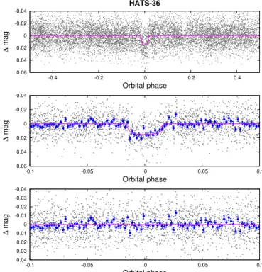
(3) The Astronomical Journal, 155:119 (14pp), 2018 March. Bayliss et al.. Table 2 Summary of HS-K2C7 Photometric Observations Target(s). Date Range. Number of Images. Cadencea (s). all all all all HATS-9 HATS-11 HATS-36 HATS-36 HATS-36 HATS579-037 (EPIC 215234145) HATS579-037 (EPIC 215234145) HATS579-037 (EPIC 215234145) HATS579-039 (EPIC 215353525). 2010 2010 2010 2015 2015 2015 2013 2014 2014 2012 2013 2015 2013. 4293 2556 3287 3754 117401 117601 137 75 80 138 194 168 67. 300 303 303 1800 60.5 60.5 130 139 139 134 130 131 211. Facility HS-1 (LCO) HS-3 (HESS) HS-5 (SSO) K2 Long Cadence (Kepler) K2 Short Cadence (Kepler) K2 Short Cadence (Kepler) PEST GROND GROND ANU2.3 m PEST PEST SWOPE. Mar–2011 Aug Mar–2011 Aug Sep–2011 Aug Oct 4–2015 Dec 2 Oct 4–2015 Dec 2 Oct 4–2015 Dec 2 Jul 1 Jul 24 Jul 28 Sept 8 Jul 7 Aug 11 Aug 20. Filter r r r Kep Kep Kep RC g, r , i, z g, r , i I RC I I. Note. a The mode time difference rounded to the nearest second between consecutive points in each light curve. Includes exposure time and overheads.. (HATS-36b), refinement of the parameters of three known HATSouth transiting planets (HATS-9b, HATS-11b, HATS12b), identification of three Jupiter-radii candidates, and classification of 18 HS-K2C7 candidates as eclipsing binaries or blended eclipsing binaries. Finally in Section 4, we discuss the results and implications of this joint ground/space-based photometry project. 2. Observations 2.1. HATSouth Photometry The HATSouth global telescope network consists of six HS4 units, two each at Siding Spring Observatory (SSO), Las Campanas Observatory (LCO), and the High Energy Spectroscopic Survey (H.E.S.S.) site. Each HS4 unit holds four Takahashi astrographs ( f/2.8, 18 cm apertures), which are each coupled to an Apogee U16M 4K×4K CCD camera. Imaging is performed using Sloan r-band filters and with exposure times of 240 s. A full description of the HATSouth telescope network hardware and operations can be found in Bakos et al. (2013). As part of the HATSouth survey (http://hatsouth.org/), we monitored a 64 square degree field (centered at 19 h 30 m00s, -2230¢00 ) between 2010 March to 2011 August. In total, we obtained 10137 images, with a cadence of approximately 300 s. In Table 2, we set out a summary of the HATSouth observations of this field, including the number of images from each site, the observation dates, and the cadence. HATSouth raw images are reduced to light curves using an automated aperture photometric pipeline detailed in Penev et al. (2013). The light curves are detrended using External Parameter Decorrelation (EPD; Bakos et al. 2010) and the Trend Filtering Algorithm (TFA; Kovács et al. 2005). These light curves are then combed for transit-like features using the box-fitting least squares algorithm (Kovács et al. 2002) with the methodology described in Bakos et al. (2004). We found 25 candidates with transit-like signals that were also were onsilicon for the K2 Campaign 7 (see Section 2.5). We designate these as “HS-K2C7 candidates,” and summarize them in Table 1. Three of these have already been published as confirmed transiting planets HATS-9b (Brahm et al. 2015), HATS-11b (Rabus et al. 2016), and HATS-12b (Rabus et al. 2016). We therefore do not discuss these further in this Section.. Figure 1. Top panel: unbinned instrumental r band light curve of HATS-36 folded with at the period P = 4.1752387 days. The solid magenta line shows the best-fit transit model (see Section 3). Middle panel: a zoom-in on the transit; the dark blue filled points here show the light curve binned in phase using a bin-size of 0.002. Lower panel: the residuals to the best-fit model.. HATSouth light curves for all stars overlapping with the K2 Campaign 7, including the HS-K2C7 candidates, are publicly available at https://hatsurveys.org/data.html. By way of example, we present the HATSouth light curve for HATS36b in Figure 1, which shows the 18 mmag transit-like dip when phase-folded at P = 4.1752387 days. The per-point rms of the HATSouth light curve for HATS-36 from the three HATSouth stations is approximately 10mmag. This is primarily shot noise from the sky background as the star is faint (V=14.386  0.020 ) as well as a small component of systematic noise on the order of 1 mmag. All HATSouth photometric data used in this paper is set out in Table 3. We 3.

(4) The Astronomical Journal, 155:119 (14pp), 2018 March. Bayliss et al.. Table 3 Differential Photometry of HS-K2C7 Candidates HS-K2C7 ID. BJD (2 400 000+). Mag. sMag. Mag (orig). Filter. Instrument. HATS-36 HATS-36 HATS-36 HATS-36 HATS-36 HATS-36 HATS-36 HATS-36 HATS-36 HATS-36. 55800.93945 55788.41475 55755.01420 55679.86013 55800.94295 55725.78922 55788.41822 55755.01796 55679.86505 55725.79268. 0.00446 −0.00216 −0.02741 0.00595 −0.00508 −0.00775 −0.00621 −0.02324 −0.00567 −0.02899. 0.01045 0.01768 0.02600 0.01239 0.00957 0.01555 0.01639 0.03203 0.01186 0.01553. L L L L L L L L L L. r r r r r r r r r r. HS HS HS HS HS HS HS HS HS HS. Note.The data are also available on the HATSouth website athttp://www.hatsouth.org. (This table is available in its entirety in machine-readable form.) Table 4 HS-K2C7 Candidate Classifications EPIC ID (HS-ID) EPIC 217671466 (HATS-9) EPIC 216414930 (HATS-11) EPIC 218131080 (HATS-12) EPIC 215969174 (HATS-36) EPIC218210199 (HATS578-002) EPIC217231249 (HATS578-003) EPIC216579956 (HATS578-004) EPIC214652580 (HATS579-001) EPIC215626177 (HATS579-007) EPIC215716837 (HATS579-008) EPIC215101303 (HATS579-009) EPIC214912104 (HATS579-010) EPIC216442060 (HATS579-014) EPIC217149884 (HATS579-015) EPIC215358983(HATS579-036) EPIC215234145 (HATS579-037) EPIC215353525 (HATS579-039) EPIC216231580 (HATS579-040) EPIC215714765 (HATS579-041) EPIC216562832 (HATS579-043) EPIC217393088 (HATS579-044) EPIC215816368 (HATS579-048) EPIC215474548 (HATS579-050) EPIC214512594 (HATS624-002) EPIC214439239 (HATS624-003). HS Recon. Teff (K). HS Recon. K (km s-1). Sec. Eclipse in K2 LC. Class.. Comment. ... ... ... 6000±300 6014  300 5928  300 5728  300 5861  300 6245  300 5334  300 6260  300 5945  300 SB2 5751  300 6700  100 5524  300 5229  212 5304  300 5645  300 6300  300 5945  300 5320  300 ... 4765  300 .... ... ... ... <2.0 -16.64  0.63 33.04  1.41 <2.0 44.22  0.81 <2.0 <2.0 20.38  2.71 <2.0 ... 13.497±0.011 22.49  0.01 <2.0 <2.0 <2.0 54.92  1.14 <2.0 <2.0 7.24  2.21 ... <2.0 .... NO NO NO NO YES YES YES YES YES YES NO YES YES YES YES NO YES NO YES YES NO NO YES YES YES. TEP TEP TEP TEP EB EB BEB EB BEB EB EB BEB EB EB EB BEB EB CAND EB EB CAND CAND EB EB BEB. HATS-9b(Brahm et al. 2015) HATS-11b(Rabus et al. 2016) HATS-12b(Rabus et al. 2016) HATS-36b (this work) ... Shallow K2 Section eclipse Blended in wide K2 apertures ... Blended in wide K2 apertures Shallow K2 Section eclipse ... Blend with nearby EB (P=43 days) Shallow K2 Section eclipse and OOT Shallow K2 Section eclipse Shallow K2 Section eclipse Color-dependent depth, K2 OOT at P=×2 K2 OOT P=3.9 days candidate (depth=1.9%) Shallow K2 Section eclipse and OOT K2 Section eclipse and OOT at P=×2 P=1.3 days candidate (depth=1.1%) P=10.1 days candidate (depth=2.5%) ... ... Blended in wide K2 apertures. note that as a result of the EPD and TFA detrending, and also due to blending from neighbors, the apparent transit depth in the HATSouth light curves is somewhat shallower than that of the true depth in the Sloanr filter (the apparent depth is typically 85% that of the true depth).. compared with a grid of synthetic templates from the MARCS model atmospheres (Gustafsson et al. 2008) in order to estimate Teff . The results for the HS-K2C7 candidates are set out in Table 4. For scheduling reasons, we obtained reconnaissance spectra for two candidates (HATS579-014 and HATS579-036) using FEROS (Kaufer et al. 1998) on the MPG 2.2 m telescope at the ESO observatory in La Silla, Chile (LSO). Spectral parameters were derived from these spectra using the CERES code (Brahm et al. 2017a) and these are also tabulated in Table 4. We note that the spectrum of HATS579-014showed that the candidate was a spectroscopic binary. We were not able to obtain a spectrum for two candidates, HATS579-050 and HATS624003, as they were too optically faint (V=16.221 and V=15.537 respectively). However, based on their 2MASS colors, apparent magnitudes, and (for HATS579-050) proper. 2.2. Reconnaissance Spectroscopy As part of the usual HATSouth program to follow-up transiting planet candidates, follow-up spectroscopy was obtained for the HS-K2C7 candidates, primarily using WiFeS (Dopita et al. 2007) on the ANU 2.3 m telescope at SSO. Full details for this observing program are given in Bayliss et al. (2013). In summary, we obtain a flux calibrated, high S/N, R = l Dl = 3000 spectrum for each candidate in order to determine the spectral type and class of the host star. These spectra are 4.

(5) The Astronomical Journal, 155:119 (14pp), 2018 March. Bayliss et al.. motion, HATS579-050 is most likely a late K-dwarf and HATS624-003 is most likely an early G-dwarf. We also use WiFeS on the ANU 2.3 m telescope to obtain multi-epoch medium resolution (R = l Dl = 7000 ) spectra to check for large amplitude (K > 2 km s-1) radial velocity variations in phase with the photometric signal. This allows us to identify candidates that are eclipsing binaries without the need of more resource-intensive high-precision radial velocity monitoring. For those targets with multi-epoch spectra, we list the measured semi-amplitudes in Table 4 assuming circular orbits. Again for the candidate HATS579-036, FEROS was used instead of WiFeS to measure the radial velocity semiamplitude. These reconnaissance radial velocity data are available on the HATSouth public archive athttp://www. hatsouth.org.. curves are plotted in Figure 3. The color-dependent depths are a strong indication that this candidate is an eclipsing binary. 3. HATS579-007 (EPIC215626177): we obtained reconnaissance photometric follow-up from the ANU2.3 m imaging camera at SSO on 2013 May 24, the imaging camera on the SWOPE 1 m at LCO on 2013 August 21, and the PEST 0.3 m PEST telescope on 2014 July 3 and 2015 August 27. None of these observations showed a transit feature. It is likely that uncertainties in the HATSouth ephemeris for this candidate were responsible for us missing the transit event for this candidate during these photometric follow-up observations. 4. HATS579-039 (EPIC215353525): we obtained reconnaissance photometric follow-up in I band from the SWOPE 1 m at LCO on 2013 August 20. A deep (25 mmag) V-shaped transit was observed, which was consistent with the r band discovery data. This observation confirmed the transit feature and refined the ephemeris for this candidate. The data for this observation are set out in Table 3.. 2.3. Reconnaissance Photometry In order to further rule out eclipsing binaries, and refine our ephemerides, we obtained ground-based photometric follow-up for four HS-K2C7 candidates. In this section, we detail all of these observations.. A summary of all photometric observations are set out in Table 2. All of the follow-up photometric data are set out in Table 3.. 1. HATS-36 (EPIC 215969174): we obtained initial photometric follow-up on the night of 2013 July 1 using the 0.3 m Perth Exoplanet Survey Telescope (PEST) in Perth, Australia. For a full description of the PEST facility see Zhou et al. (2014) and the PEST website (http:// pestobservatory.com). Imaging was carried out in the RC band with exposure times of 120 s. In total, 137 exposures of HATS-36 were taken. Data was reduced via aperture photometry as described in Zhou et al. (2014). The resulting light curve is plotted in Figure 2 and the data is provided in Table 3. A full transit is clearly detected with a depth and duration consistent with the HATSouth discovery data. These data allowed us to refine the transit ephemeris. The following year, we observed two consecutive partial transits of HATS-36b with the multiband GROND imager (Greiner et al. 2008) on the MPG 2.2 m telescope at LSO in Chile. On the night of 2014 July 24, we observed a transit egress (75×110 s images in g , r , i, z band), while on the night of 2014 July 28, we observed a transit ingress (80×110 s images in g , r , i band). These data were reduced to light curves via aperture photometry following the method set out in Mohler-Fischer et al. (2013). The light curves are plotted in Figure 2 and the data is set out in Table 3. These highprecision light curves confirmed the transit depth was color independent and were consistent with a transiting planet. Both the PEST and GROND light curves for HATS-36 are used in the global fitting described in Section 3. 2. HATS579-037(EPIC215234145): we obtained reconnaissance photometric follow-up from the ANU2.3 m imaging camera at SSO on 2012 September 8 in I band, which showed a “V”-shaped transit with a depth of 20 mmag (compared with the 10 mmagtransit observed in the HATSouth discovery data). This color-dependent depth difference was confirmed with observations from the PEST 0.3 m telescope, which observed a 10 mmagtransit in RC band on 2013 July 7, and a 20 mmagtransiting IC band on 2015 August 11. These depth differences are statistically significant at a >3s -level. The photometric data for this candidate is set out in Table 3, while the follow-up light. 2.4. High-resolution Spectroscopy—Radial Velocities We obtain radial velocity measurements for HS-K2C7 candidates that remain after the reconnaissance spectroscopy and photometry set out in Sections 2.2 and 2.3 respectively. An additional magnitude constraint of V<14.5 is placed on candidates at this stage, as the radial velocity monitoring of candidates fainter than V=14.5 is beyond the reach of most telescopes/instruments. Only in exceptional cases such as an M-dwarf host (e.g., HATS-6b; Hartman et al. 2015) do we attempt high-precision radial velocity measurements for such faint candidates. By this criteria, just seven candidates remained: three of which have already been published (HATS-9b, HATS-11b, and HATS-12b) and four which are presented below: 1. HATS-36 (EPIC 215969174): We measured the radial velocity of HATS-36 using FEROS on the MPG2.2 m at LSO between 2013 July 16 and 2014 July 24. In total, 16 measurements were made spread over the phase of the photometric period (4.1752 day). These data were reduced using the CERES FEROS echelle spectrograph pipeline described in Brahm et al. (2017a). We find a radial velocity variation in phase with the photometric period and with an amplitude of K=356.9  3.6 m s-1, indicating the transiting companion was of a planetary mass. We present these radial velocity data in Table 5 and plot the data along with a best-fit circular orbit in Figure 4. These data are used in Section 3 to model the global parameters of the system— primarily determining the mass of the transiting planet. 2. HATS579-007 (EPIC215626177): We obtained multiple high-resolution spectra of this target from several different instruments; however, the data showed no radial velocity variation above 10 m s-1. Coupled with the lack of a transit in the reconnaissance photometry (see Section 2.3), we put the monitoring of this candidate on hold until K2 data became available (see Section 2.5). 5.

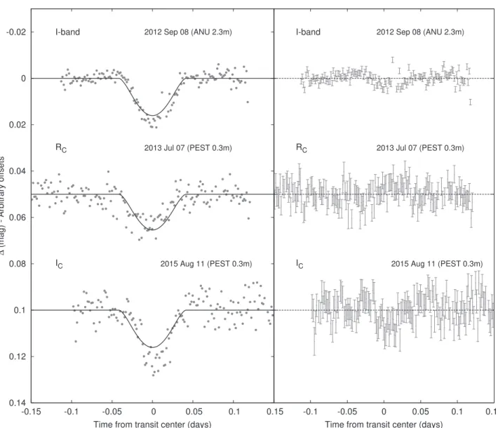
(6) The Astronomical Journal, 155:119 (14pp), 2018 March. Bayliss et al.. Figure 2. Left: unbinned ground-based follow-up transit light curves of HATS-36. The dates, filters, and instruments used for each event are indicated. The light curves have been detrended using the EPD process. Curves after the first are shifted for clarity. Our best fit is shown by the solid red lines. Right: residuals from the fits in the same order as the curves at left.. 7 monitored a field centered on 19 h 11m 19s, -2321¢36. As this K2 field overlapped with the previously monitored HATSouth field described in 2.1, we were able to obtain K2 data for the 25 HS-K2C7 candidates listed in Table 2 via the K2 Guest Observer programs GO7066 and GO7067. A summary of the K2 imaging is set out in Table 1. The K2 data was made available on 2016 April 20. We used three different versions of the K2 light curves downloaded from the Mikulski Archive for Space Telescopes (http://archive. stsci.edu). We used the K2 PDC light curves, the light curves produced by the “self-flat-fielding” technique described in Vanderburg & Johnson (2014), and the K2 light curves from the EVEREST open-source pipeline fully described in Luger et al. (2016, 2017). In addition, we used the K2SC light curves (Aigrain et al. 2016) that were provided to us upon request (B. Pope 2016, private communication). All four of these data products are derived from the same raw pixel data. However, the different apertures and detrending techniques result in light curves with sometimes quite marked differences. We therefore analyzed all four in order to help. 3. HATS579-015 (EPIC217149884): We obtained four FEROS observations for this candidate between 2016 May 18 and 2017 May 31. The observations show an in-phase radial velocity variation with K = 13.497  0.011 km s-1, indicating the companion is of stellar mass and the candidate is therefore an eclipsing binary. 4. HATS579-037 (EPIC215234145): We obtained multiple high-resolution spectra of this target from several different instruments; however, the data showed no radial velocity variation above 10 m s-1. Due to this lack of variation, along with the color-dependent transit depths (see Section 2.3), we put this candidate on hold until K2 data became available (see Section 2.5). 2.5. K2 Photometry The K2 mission (Howell et al. 2014) uses the Kepler space telescope (Borucki et al. 2010) to monitor selected fields in the ecliptic plane for campaigns of approximately 80 days each. Between 2015 October 4 and 2015 December 2, K2 Campaign 6.

(7) The Astronomical Journal, 155:119 (14pp), 2018 March. Bayliss et al.. Figure 3. Left: unbinned ground-based follow-up transit light curves of HATS579-037. Plots as for Figure 2. The over-plotted model is based on a global fit of all available data, and accounts for differences in limb darkening between the R- and i-bands, but assumes all other light curve parameters are the same. The poor fit of this model shows clear differences in the observed transit depths between the R-band and i-band observations, which allow us to classify this candidate as a eclipsing binary.. Due to the space-based environment, the large aperture (1 m), and near continuous 80 day coverage, all of the K2 light curves we used are of very high precision—for K2 Campaign 7, the median 6.5 hr combined differential photometric precision (CDPP) for a Kp=12 mag dwarf star was 120 ppm. With this very high precision, we are able to see features not visible or ambiguous in the HATSouth discovery light curves. Most importantly, we can search for secondary eclipses, out-of-transit ellipsoidal variation, and odd/even transit depth differences. These features, in an optical light curve and at significant amplitudes, are characteristic of eclipsing binary systems rather than transiting exoplanets. The timing was such that the K2 observations and data followed after we had already completed the photometric and spectroscopic follow-up of the HS-K2C7 candidates detailed in Sections 2.3, 2.2, and 2.4. In this respect, some candidates had already been robustly identified as either transiting exoplanets or eclipsing binaries before the K2 data was analyzed.. categorize our HS-K2C7 candidates. Each HS-K2C7 candidate was detrended individually to take into account the fact that each light curve potentially contained a combination of K2 systematics, variability due to stellar rotation, and ellipsoidal variability. We detrended the light curves by first masking the transit/eclipse signal, and then flattening the curve using a fifth order SavitzkyGolay filter (Savitzky & Golay 1964), with the window length selected to detrend variations due to K2 systematics and variability due to stellar rotation, but to avoid flattening any potential ellipsoidal variation or secondary eclipse. The resulting 25 light curves are presented in Figure 5. In most instances, we utilized the Everest light curves; however, for some light curves the Everest algorithm removed real astrophysical variability, so in those cases we used the PDC light curves. Features seen in these light curves, such as secondary eclipses and out-of-transit variability, are noted in Table 4. 7.

(8) The Astronomical Journal, 155:119 (14pp), 2018 March. Bayliss et al.. Table 5 Relative Radial Velocities and Bisector Span Measurements of HATS-36 BJD (2, 450, 000+). RVa (m s-1). sRV b (m s-1). BS (m s-1). sBS. Phase. Instrument. 6489.79353 6492.81654 6841.72454 6842.59071 6844.76223 6846.77951 6847.58993 6852.66976 6852.82588 6853.77517 6855.59317 6856.83423 6857.73972 6858.64854 6859.67881 6862.65477. −113.43 −302.03 328.57 47.37 −57.83 29.47 −226.73 −315.43 −232.63 294.77 −140.43 −291.33 199.17 327.37 −121.03 424.37. 15.60 17.90 15.00 20.00 13.30 13.30 15.30 18.40 19.60 21.50 16.30 16.40 14.20 13.90 16.60 26.90. −3.0 42.0 37.0 4.0 31.0 13.0 2.0 109.0 86.0 58.0 10.0 −76.0 38.0 4.0 13.0 141.0. 17.0 18.0 16.0 21.0 15.0 15.0 15.0 16.0 16.0 19.0 17.0 17.0 15.0 15.0 18.0 26.0. 0.486 0.210 0.776 0.983 0.503 0.987 0.181 0.397 0.435 0.662 0.097 0.395 0.612 0.829 0.076 0.789. FEROS FEROS FEROS FEROS FEROS FEROS FEROS FEROS FEROS FEROS FEROS FEROS FEROS FEROS FEROS FEROS. Notes. a The zero-point of these velocities is arbitrary. An overall offset grel fitted separately to the FEROS velocities in Section 3 has been subtracted. b Internal errors excluding the component of astrophysical/instrumental jitter considered in Section 3.. Figure 5. Two of the 24 K2 light curves for the HS-K2C7 candidates. The full set is available in the online Figure set. Light curves are from Everest (EV) or the K2 PDC pipeline (PDC). Classifications are transiting exoplanet (TEP), candidate (CAND), eclipsing binary (EB) or blended eclipsing binary (BEB). (The complete figure set (24 images) is available.). Figure 4. Top panel: high-precision RV measurements for HATS-36 from MPG 2.2 m/FEROS, together with our best-fit circular orbit model. Zero phase corresponds to the time of mid-transit. The center-of-mass velocity has been subtracted. Middle panel: velocity O - C residuals from the best-fit model. The error bars for each instrument include the jitter, which is varied in the fit. Bottom panel: bisector spans (BS), with the mean value subtracted. Note the different vertical scales of the panels.. Figure 6. K2 Kep band light curve (EVEREST) of HATS-36 folded with the period P = 4.1752387 days resulting from the global fit described in Section 3. The top panel shows the full phase-wrapped light curve. The middle panel shows a zoom-in on the transit. The lower panel shows a zoom around phase 0.5 with no detection of a secondary eclipse. Points are individual K2 measurements. The black solid line is the best-fit global model described in Section 3.. However, in other cases the K2 data were critical to our classification of the candidate. Here, we detail the findings for each HS-K2C7 candidate. 8.

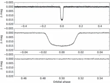
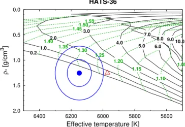
(9) The Astronomical Journal, 155:119 (14pp), 2018 March. Bayliss et al.. 1. HATS-36 (EPIC 215969174): The phase-folded K2 light curve for HATS-36 is presented in Figure 6, and the data is tabulated in Table 3. It shows a 15 mmag U-shaped transit consistent with the discovery and follow-up photometry presented in Sections 2.1 and 2.3, respectively. There is no secondary eclipse, odd/even depth difference, or out-oftransit variation present to the limits of the photometry. This light curve is used in our global analysis of this newly discovered transiting exoplanet system in Section 3. 2. Known HATSouth Planets: The K2 data for HATS-9, HATS-11, and HATS-12 are consistent with the previous published exoplanet discoveries—i.e., there was no evidence of any secondary eclipses, odd/even depth differences, or out-of-transit variations. We analyze these light curves for additional planets, TTVs and phase modulations in Section 3. 3. HATSouth Candidates: HATS579-040, HATS579-044, and HATS579-048 all have K2 light curves that are consistent with the HATSouth discovery data with no sign of secondary eclipses, odd/even depth differences, or outof-transit variations. The light curves are set out in Figure 5. 4. Eclipsing Binaries: The 18 remaining HS-K2C7 candidates are eclipsing binaries. There are 16 candidates that show secondary eclipses in the K2 light curves indicating they are eclipsing binaries. The details for each candidate are set out in Table 4, and the light curves are set out in Figure 5. For HATS579-009, we do not detect a secondary eclipse; however, we detected a high-amplitude (K=20 km s-1) in-phase radial velocity variation (see Section 2.4) indicating it is an eclipsing binary. Likewise, HATS579-037 does not have a detectable secondary eclipse; however, it had color-dependent transit depths (see Figure 3) and the K2 light curve also shows out-of-transit variation when phase-folded at ×2 the discovery period. Therefore, we classify this candidate as a eclipsing binary.. Figure 7. Comparison between the measured values of Teff and r (from ZASPE applied to the FEROS spectra, and from our modeling of the light curves and RV data, respectively), and the Y2 model isochrones from Yi et al. (2001). The best-fit value (dark blue filled circle), and approximate 1σ and 2σ confidence ellipsoids are shown. The value from our initial ZASPE iteration is shown with an open red triangle. Black solid lines show the Y2 isochrones for ages indicated (0.2 to 10.0 Gyr). The green dashed lines show evolutionary tracks for stars with masses indicated in solar mass units.. the physical stellar parameters. Figure 7 shows the final log g value plotted against Teff , with 1σand 2σconfidence ellipsoids and the appropriate Y2 isochrones for various stellar ages. The final parameters indicate that HATS-36 is a G0V dwarf star (Teff = 5970  160 K, log g = 4.400  0.023) with a mass and radius of M = 1.155  0.039 M☉ and R  = 1.222  0.029 R☉, respectively. The metallicity is slightly above solar with [Fe H] = 0.280  0.037. The rotational velocity (v sin i = 4.98  0.29 km s-1) and age (0.62 0.55 Gyr) are not atypical for a star of this type and class. The full list of final stellar parameters are set out in Table 6. To exclude blended eclipsing binary scenarios for HATS36b, we carried out an analysis of all the data following the methodology set out in Hartman et al. (2012). We model the photometric data, including the K2 observations, as an eclipsing binary system blended with a third star. The stars in the model are constrained using the Padova isochrones (Girardi et al. 2000), and also must have a blended spectrum consistent with the determined atmospheric parameters. We also simulate composite cross-correlation functions (CCFs) and use them to predict radial velocities and bisector spans for each blend scenario. All blend models tested can be rejected with >6s confidence based on the photometry alone. Moreover, none of the blend models tested would produce RV variations or non-variable bisectors consistent with the observations. To determine the properties of HATS-36b, we globally model the photometric and spectroscopic data following Pál et al. (2008), Bakos et al. (2010), and Hartman et al. (2012). We fit Mandel & Agol (2002) transit models to the light curves, and a Keplerian orbit is fit to the radial velocity measurements presented in Section 2.4, allowing for RV jitter. For the groundbased light curves, we fixed the quadratic limb-darkening coefficients to tabulated values based on the stellar atmospheric parameters, while for the K2 light curve, we allowed the quadratic limb-darkening coefficients to vary in the fit. For the long-cadence K2 observations, we made use of the EVEREST light curves, with the transit model numerically integrated over. 3. Analysis In this section, we analyze the newly discovered transiting exoplanet HATS-36b, the three known HATSouth with K2 data (HATS-9b, HATS-11b, and HATS-12b), and the three HS-K2C7 targets that remain as transiting exoplanet candidates. 3.1. HATS-36b: A High-mass, Eccentric, Transiting Hot Jupiter To derive the physical properties of HATS-36, we obtain initial stellar parameters from the high-resolution spectra of HATS-36 from FEROS, together with ZASPE (Brahm et al. 2017b). This provides a first estimate of the temperature (Teff ), surface gravity (log g ), metallicity ([Fe H]), and projected equatorial rotation velocity (v sin i ) of HATS-36. The Teff and [Fe H] values are then used with the stellar density r , determined from the combined light-curve and radial velocity analysis, to determine a first estimate of the stellar physical parameters following the method described in Sozzetti et al. (2007). We use the Yonsei–Yale isochrones (Y2; Yi et al. 2001) to derive the stellar mass, radius, and age that best fit our estimated Teff , [Fe H] and r values. We then determine a revised value of log g and perform a second iteration of ZASPE holding log g fixed to this value while fitting for Teff , [Fe H], and v sin i . We again compare this new value of r to the Y2 isochrones to produce our final adopted values for 9.

(10) The Astronomical Journal, 155:119 (14pp), 2018 March. Bayliss et al.. Table 6 Stellar Parameters for HATS-36 Parameter. Value. Astrometric properties and cross-identifications 2MASS-IDK 2MASS19255488-2312100 K2-IDK EPIC 215969174 (K2-145) 19 h25m 54.s 84 R.A. (J2000)K -2312¢10. 0 Decl. (J2000)K -1.5  3.0 m R.A. (mas yr-1) -7.5  3.0 m Decl. (mas yr-1) Spectroscopic properties 6149  76 Teff (K)K 0.280  0.037 [Fe H]K 4.98  0.29 v sin i (km s-1)K -24.392  31 gRV (km s-1)K Photometric properties 15.060  0.030 B (mag)K 14.386  0.020 V (mag)K 14.675  0.010 g (mag)K 14.231  0.010 r (mag)K 14.146  0.050 i (mag)K 14.300  0.030 Kep (mag)K 14.148  0.013 G (mag)K 13.181  0.026 J (mag)K 12.855  0.025 H (mag)K 12.809  0.026 Ks (mag)K Derived properties 1.222  0.029 M (M☉ )K 1.155  0.039 R  (R☉)K 1.26  0.27 r (g cm-3)b K 1.118  0.091 r (g cm-3)b K. 4.400  0.023 1.64  0.17 4.24  0.12 2.897  0.083 0.62  0.55 0.232  0.060 962  37. log g (cgs)K L  (L ☉ )K MV (mag)K MK (mag,ESO) Age (Gyr)K AV (mag)K Distance (pc)K. Table 7 Parameters for the Transiting Planet HATS-36b Sourcea. Parameter Light curve parameters P (days) K Tc (BJD ) K T14 (days) K T12 = T34 (days) K a R  K z R  K Rp /R  K b2 K b º a cos i R  K i (deg) K Limb-darkening coefficients c1, i (linear term) K c2 , i (quadratic term) K c1, r K c2 , r K c1, kep K c2 , kep K RV parameters K (m s-1) K e K RV jitter (m s-1) K Planetary parameters Mp (MJ ) K Rp (RJ ) K C (Mp, Rp ) K rp (g cm-3) K. 2MASS 2MASS UCAC4 UCAC4 ZASPE ZASPE ZASPE FEROS APASS APASS APASS APASS APASS EPIC Gaia DR1 2MASS 2MASS 2MASS Y2+r +ZASPE Y2+r +ZASPE Light curves Y2+Light curves +ZASPE Y2+r +ZASPE Y2+r +ZASPE Y2+r +ZASPE Y2+r +ZASPE Y2+r +ZASPE Y2+r +ZASPE Y2+r +ZASPE. log gp (cgs) K a (AU) K Teq (K) K Θ K áF ñ (108 erg s-1 cm-2 ) K. (å. ci (t - T0 )i +. Nharm (a j , k k= 1. å j=1. NMorlet -0.5 ((t - tj ) s )2 e. cos ((t - T0) kn ) + bj, k sin ((t - T0) kn )). ). 0.2234 0.3621 0.3057 0.3623 0.335±0.051 0.291±0.090 356.9  3.6 0.105  0.028 15  44 3.216  0.062 1.235  0.043 0.61 2.12  0.20 3.718  0.026 0.05425  0.00043 1356  30 0.2307  0.0082 7.64  0.69. where t is the time of observation, T0 is a fixed reference epoch, tj are a fixed evenly spaced set of times for centering the wavelets, σ is a fixed wavelet width which we set equal to tj + 1 - tj , ν is fixed to the dominant quasi-periodic frequency, and ci, aj, k , and bj, k are linearly optimized parameters in the model. For our analysis of HATS-36b, we adopted Npoly = 2, NMorlet = 7, and Nharm = 4. The resulting K2 light curve is shown in Figure 6, while the data are part of the photometry set presented in Table 3. The model is fit simultaneously with the transit model as part of the global analysis. We use a Differential Evolution Markov Chain Monte Carlo procedure to determine the posterior distribution of the parameters. We find a statistically significant non-zero eccentricity of e = 0.105  0.028; hence, we do not assume a circular orbit for this system. The planetary parameters resulting from this global fit are set out in Table 7. HATS-36b is a high-mass (Mp = 3.216  0.062 MJ ), Jupiter-sized (Rp = 1.235  0.043 RJ ) transiting planet with an orbital period of 4.1752387  0.0000022 days. It has a bulk density of 2.12  0.20 g cm-3.. the exposure times. This light curve showed large amplitude quasi-periodic variations, likely due to a combination of lowfrequency systematic errors in the K2 photometry, and the rotational modulation of stellar active regions on the surface of HATS-36. We discuss the stellar activity signature later in this section. In order to model these variations in our analysis, we made use of a Morlet-type wavelet basis and a low order polynomial. This model has the form: Npoly. 4.1752387  0.0000022 2457360.390330  0.000085 0.14428  0.00078 0.01753  0.00076 10.10  0.28 +0.086 15.7490.065 0.10966  0.00067 +0.029 0.2040.034 +0.031 0.4520.040 87.61  0.23. Note. For each parameter, we give the median value and 68.3% (1σ) confidence intervals from the posterior distribution. Detailed notes on parameters can be found in Table 6 of Espinoza et al. (2016).. Notes. a 2MASS (Skrutskie et al. 2006), APASS (Henden et al. 2009), Gaia (Lindegren et al. 2016), ZASPE=Zonal Atmospherical Stellar Parameter Estimator routine for the analysis of high-resolution spectra (Brahm et al. 2017b), Y2 isochrones (Yi et al. 2001). b In the case of r , we list two values. The first value is determined from the global fit to the light curves and radial velocity data, without imposing a constraint that the parameters match the stellar evolution models. The second value results from restricting the posterior distribution to combinations of r +Teff +[Fe H] that match to a Y2 stellar model.. å i=0. Value. (1 ). 10.

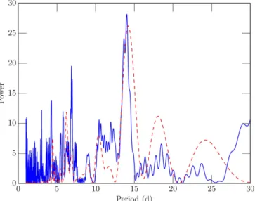
(11) The Astronomical Journal, 155:119 (14pp), 2018 March. Bayliss et al.. methodology described in those papers and in Section 3.1. Here, we make use of the (Espinoza et al. 2016) light curves rather than the EVEREST light curves, and we apply filter lowfrequency variations due to stellar activity and instrumental errors prior to fitting the transit model. For HATS-9b and HATS-11b, short cadence data was available, and we made use of these observations, rather than the long cadence, in our analysis. The results allow us to improve the precision for the planetary parameters for these systems, and we list these in Table 8. Most of the revisions to the planetary parameters are relatively minor. The largest change is for the radius of HATS9b, which is revised upwards by almost 10%. This is primarily due to the limited photometric follow-up that was available when the parameters of HATS-9b were calculated in the original analysis of Brahm et al. (2015). For the case of HATS-11b, our global modeling, assuming a circular orbit, also finds a secondary eclipse with a planet-tostar flux ratio of 0.0032±0.0012. In addition to improving the parameters for these planets, we utilize the K2 light curves to search for additional transiting planets. The discoveries of WASP-47d and WASP-47e (Becker et al. 2015) show that hot Jupiters can have nearby planetary neighbors. After removing the transit events from the hot Jupiters, we search the K2 light curves of HATS-9, HATS-11, and HATS-12, using the BLS search algorithm as discussed in Section 2.1. We do not find any significant evidence for additional transiting planets in any of these systems. Using the original light curves and the K2 data, we check for any changes in the timing of the transits for these exoplanets. We do this by fitting the best-fit transit model (using the parameters set out in Table 8) to each individual transit event and measuring the difference between the best-fit central transit time and the expected transit time from a purely Keplerian orbit. For all three systems, we find no evidence of any transit timing variations. Finally, we analyze the K2 light curves for evidence for of additional variability. HATS-11 and HATS-12 only show longterm drift in the K2 data that is likely caused by systematics from the spacecraft. HATS-9 shows an additional modulation with a period of approximately 8.8days and a peak-to-peak amplitude of approximately 0.1%. If this modulation is indeed due to stellar rotation, it would imply an equatorial rotation of ve = 8.6 km s-1. Given the spectroscopic v sin i of HATS-9 is 4.58  0.90 km s-1, this would mean the spin axis of the star is inclined with respect to our line of sight, and that the planet is on a misaligned orbit.. Figure 8. The power spectrum from a Lomb–Scargle analysis of the HATSouth photometry (blue solid line) and the K2 photometry (red dashed line) for HATS-36. The peak at ∼14 days is the likely rotational period of the star and is prominent in both data sets.. From our radial velocity monitoring, we robustly measure a non-zero eccentricity (e = 0.105  0.028). This is not entirely surprising, as it has been noted that massive hot Jupiters (Mp > 2 MJ ) often show non-zero eccentricity (Turner et al. 2016). Indeed, HATS-36b is very similar in orbital period and eccentricity to HATS-22b (Bento et al. 2017) and HAT-P-14b (Torres et al. 2010), both of which are massive hot Jupiters at 2.7 and 2.2 MJ , respectively. Given the young age of the HATS-36b system (0.62  0.55 Gyr), it is entirely possible that the planet has not had time to tidally circularize as is thought to have occurred for other lower mass and older hot Jupiter systems. We take the raw (pre-detrending) HATS-36 K2 light curve (Vanderburg & Johnson 2014), remove the transit events, and examine the longer timescale variability using a Lomb Scargle analysis. From this analysis, we detect a strong modulation at 14.4days with a peak-to-peak amplitude of approximately 0.5%. Such a rotational period is typical for a star of the spectral type and class of HATS-36 (McQuillan et al. 2014). We confirm this rotational signal is also present in the HATSouth discovery light curve, again showing modulation at P=14days. The Lomb–Scargle power spectrum is presented in Figure 8 for both the K2 data and the HATSouth data. Assuming R  = 1.155  0.039, this rotation period would result in an equatorial rotational of ve = 4.17 km s-1, in contrast the spectroscopic derived v sin i = 4.98  0.29 km s-1. The fact that the derived rotational period is 2 - s below the spectroscopic v sin i may be a sign that we have picked up a harmonic of the rotational period rather than the true rotational period. Alternatively, it may be due to non-equatorial spots and solarlike differential rotation.. 3.3. Candidates Three of the HATSouth candidates from the HS-K2C7 campaign remain viable transiting exoplanet candidates, but have not been confirmed via radial velocity measurements due to the faintness of the host stars. In this Section, we discuss the details for each candidate.. 3.2. HATS-9b,11b,12b. 1. HATS579-040(EPIC216231580): The transiting candidate has a period of P=3.905 days and shows a 17 mmag “U”-shaped transit. The host star is a faint (V=14.963) G9 dwarf (Teff = 5304  300 K). Assuming a host star mass of 0.9 M , and with a radial velocity semi-amplitude of K<2.0 km s-1, we can constrain the companion mass to be less than 15 MJ for an unblended. High-precision K2 data allowed us to revisit the three transiting exoplanets already published by the HATSouth team, namely HATS-9b (Brahm et al. 2015) and HATS-11b and HATS-12b (Rabus et al. 2016). We augment our originally published photometric and spectroscopic data with the new K2 photometry and re-run the global modeling with the 11.

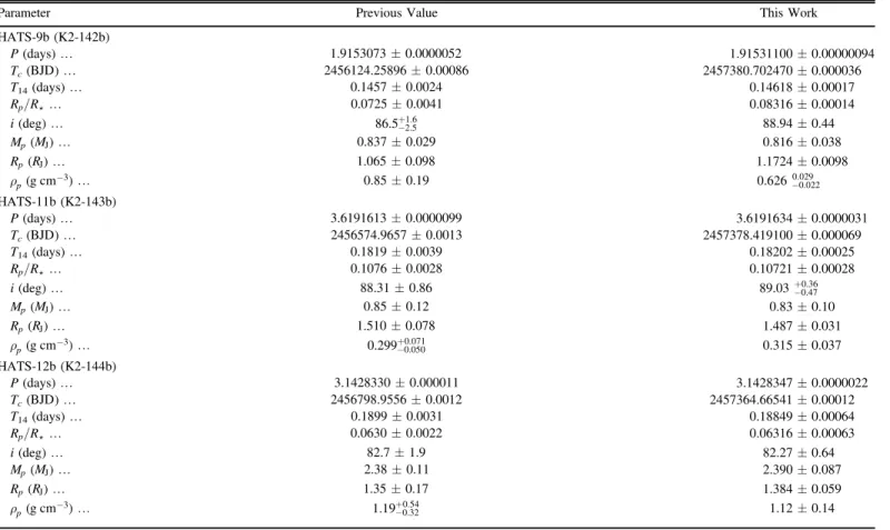
(12) The Astronomical Journal, 155:119 (14pp), 2018 March. Bayliss et al. Table 8 Updated Planet Parameters Previous Value. This Work. HATS-9b (K2-142b) P (days) K Tc (BJD ) K T14 (days) K Rp /R  K i (deg) K Mp (MJ ) K Rp (RJ ) K rp (g cm-3) K. Parameter. 1.9153073  0.0000052 2456124.25896  0.00086 0.1457  0.0024 0.0725  0.0041 +1.6 86.52.5 0.837  0.029 1.065  0.098 0.85  0.19. 1.91531100±0.00000094 2457380.702470±0.000036 0.14618±0.00017 0.08316±0.00014 88.94±0.44 0.816±0.038 1.1724±0.0098 0.626 -0.029 0.022. HATS-11b (K2-143b) P (days) K Tc (BJD ) K T14 (days) K Rp /R  K i (deg) K Mp (MJ ) K Rp (RJ ) K rp (g cm-3) K. 3.6191613  0.0000099 2456574.9657  0.0013 0.1819  0.0039 0.1076  0.0028 88.31  0.86 0.85  0.12 1.510  0.078 +0.071 0.2990.050. 3.6191634±0.0000031 2457378.419100±0.000069 0.18202±0.00025 0.10721±0.00028 +0.36 89.03 0.47 0.83±0.10 1.487±0.031 0.315±0.037. HATS-12b (K2-144b) P (days) K Tc (BJD ) K T14 (days) K Rp /R  K i (deg) K Mp (MJ ) K Rp (RJ ) K rp (g cm-3) K. 3.1428330  0.000011 2456798.9556  0.0012 0.1899  0.0031 0.0630  0.0022 82.7  1.9 2.38  0.11 1.35  0.17 +0.54 1.190.32. 3.1428347±0.0000022 2457364.66541±0.00012 0.18849±0.00064 0.06316±0.00063 82.27±0.64 2.390±0.087 1.384±0.059 1.12±0.14. single-host/single companion system. Gaia DR1 (Lindegren et al. 2016) shows a single source (G = 14.702) having no neighbors within 15″down to the Gaia DR1 magnitude limit (G ~ 20) and separation limit (∼1″). 2. HATS579-044(EPIC217393088): The transiting candidate has a period of P=1.320 days and shows a 10 mmag “U”-shaped transit. The host star is faint (V=15.575) G0 dwarf (Teff = 5945  300 K). Assuming a host star with 1.1 M , and with a radial velocity semi-amplitude of K<2.0 km s-1, we can constrain the companion mass to be less than 11.5 MJ for an unblended single-host/single companion system. Gaia DR1 shows the host is a single source (G = 15.288), having no neighbors within 15″. 3. HATS579-048(EPIC215816368): The transiting candidate has a relatively long period of P=10.148 days and shows a 20 mmag “U”-shaped transit. The host star is a faint (V=15.835) G9 dwarf (Teff = 5320  300 K). Assuming a host star mass of 0.9 M , with a radial velocity semi-amplitude of K 7.24  2.21 km s-1, we would determine a companion mass of 70 MJ -approximately at the lower limit for H-burning. If confirmed, this would join the small population of known transiting brown dwarfs, and would follow the trend of having a longer orbital period than typical hot Jupiters (Bayliss et al. 2017). From the Gaia DR1, we see a primary source (G = 15.610), with a neighbor at 9 5 (G = 18.182). However, by analyzing multiple pixel-aperture sizes from the SFF K2 light curves (Vanderburg & Johnson 2014), we determine the detected transit signal originates from. the primary candidate star rather than the fainter neighbor.. 4. Discussion This is the first time we have vetted HATSouth candidates using the high-precision photometry afforded by the Kepler telescope, although it has been done for HATNet under K2 program GO0116 (PI Bakos) resulting in the discovery of HAT-P-56b (Huang et al. 2015). In the cases of both HATS36b and HAT-P-56b, the radial velocity semi-amplitudes are high (∼300 m s-1), but the stellar jitter is also high (∼100 m s-1), and thus the K2 data is especially helpful in robustly confirming the nature of the systems.. 4.1. HATS-36b HATS-36b is a hot Jupiter with a typical orbital period (P=4.1752387  0.0000022 days). The star is active, which we see manifest in the the variability of the K2 light curve and the rotational periodicity recovered from the HATSouth light curve. It has a moderate but well-measured eccentricity, which is consistent with other high-mass hot Jupiters with measured eccentricities. Due to its high mass, HATS-36b lies in a relatively sparsely populated region of the mass-density relationship for gas giant exoplanets (see Figure 9). However, its bulk density fits well on the mass-density sequence of gas giants. 12.

(13) The Astronomical Journal, 155:119 (14pp), 2018 March. Bayliss et al.. FONDECYT project 1171208, BASAL CATA PFB-06, and project IC120009 “Millennium Institute of Astrophysics (MAS)” of the Millennium Science Initiative, Chilean Ministry of Economy. N.E. is supported by CONICYT-PCHA/Doctorado Nacional. R.B. and N.E. acknowledge support from project IC120009 “Millennium Institute of Astrophysics (MAS)” of the Millennium Science Initiative, Chilean Ministry of Economy. V. S. acknowledges support form BASAL CATA PFB-06. A.V. is supported by the NSF Graduate Research Fellowship, grant No. DGE 1144152. This paper includes data collected by the K2 mission. Funding for the K2 mission is provided by the NASA Science Mission directorate. The K2 observations presented here were obtained through the GO program, with analysis supported by NASA grant NNX16AE68G. This work is based on observations made with ESO Telescopes at the La Silla Observatory. This paper also uses observations obtained with facilities of the Las Cumbres Observatory Global Telescope. We acknowledge the use of the AAVSO Photometric All-Sky Survey (APASS), funded by the Robert Martin Ayers Sciences Fund, and the SIMBAD database, operated at CDS, Strasbourg, France. Operations at the MPG2.2 m Telescope are jointly performed by the Max Planck Gesellschaft and the European Southern Observatory. The imaging system GROND has been built by the high-energy group of MPE in collaboration with the LSW Tautenburg and ESO. We thank the MPG 2.2 m telescope support team for their technical assistance during observations.. Figure 9. Mass-density relationship of all well-characterized (density uncertainty <20%) giant exoplanets. Blue circles are data from NASA Exoplanet Archive (2016 November 23) and the red square is HATS-36b.. 4.2. Candidates Secondary eclipses in K2 allow us to robustly rule out 17 of the 25 HS-K2C7 candidates. However, we have three candidates that remain active. All three candidates require future radial velocity monitoring in order to determine if they are transiting exoplanets/brown dwarfs or (blended) eclipsing binaries. However, such a task is extremely difficult to due to faintness of the host stars. HATS579-048 (EPIC215816368) is the most promising, as we have an indication of a velocity variation of K=7.24  2.21 km s-1. However, the host star is also the faintest of the three candidates at V=15.835.. ORCID iDs D. Bayliss https://orcid.org/0000-0001-6023-1335 J. D. Hartman https://orcid.org/0000-0001-8732-6166 G. Zhou https://orcid.org/0000-0002-4891-3517 G. Á. Bakos https://orcid.org/0000-0001-7204-6727 A. Vanderburg https://orcid.org/0000-0001-7246-5438 R. Brahm https://orcid.org/0000-0002-9158-7315 A. Jordán https://orcid.org/0000-0002-5389-3944 N. Espinoza https://orcid.org/0000-0001-9513-1449 M. Rabus https://orcid.org/0000-0003-2935-7196 T. G. Tan https://orcid.org/0000-0001-5603-6895 K. Penev https://orcid.org/0000-0003-4464-1371 W. Bhatti https://orcid.org/0000-0002-0628-0088 M. de Val-Borro https://orcid.org/0000-0002-0455-9384 V. Suc https://orcid.org/0000-0001-7070-3842. 4.3. Outlook This program shows the benefit of using high-precision K2 space-based photometry to vet candidates identified from ground-based surveys. This concept will naturally extend to the TESS mission (Ricker et al. 2014). The primary differences will be twofold. First, TESS will monitor most stars for only 27 days, about one-third the duration of the K2 campaigns. For many of our HS-K2C7 candidates, such duration would result in only one or two transits to be observed. In these cases, the value of combining the TESS data with ground-based monitoring is greatly enhanced. Second, the spatial resolution of TESS is just 21. 1 pixel−1, meaning many blended systems that can be resolved in K2, such as the blended eclipsing binaries presented in this work, will not be readily identifiable from TESS data alone. In these cases, ground-based data such as that from HATSouth (3. 7 pixel−1) will be highly beneficial in resolving the nature of the systems.. References Aigrain, S., Parviainen, H., & Pope, B. J. S. 2016, MNRAS, 459, 2408 Bakos, G., Noyes, R. W., Kovács, G., et al. 2004, PASP, 116, 266 Bakos, G. Á, Csubry, Z., Penev, K., et al. 2013, PASP, 125, 154 Bakos, G. Á, Torres, G., Pál, A., et al. 2010, ApJ, 710, 1724 Barge, P., Baglin, A., Auvergne, M., et al. 2008, A&A, 482, L17 Bayliss, D., Hojjatpanah, S., Santerne, A., et al. 2017, AJ, 153, 15 Bayliss, D., Zhou, G., Penev, K., et al. 2013, AJ, 146, 113 Becker, J. C., Vanderburg, A., Adams, F. C., Rappaport, S. A., & Schwengeler, H. M. 2015, ApJL, 812, L18 Bento, J., Schmidt, B., Hartman, J. D., et al. 2017, MNRAS, 468, 835 Borucki, W. J., Koch, D., Basri, G., et al. 2010, Sci, 327, 977 Brahm, R., Jordán, A., & Espinoza, N. 2017a, PASP, 129, 034002 Brahm, R., Jordán, A., Hartman, J., & Bakos, G. 2017b, MNRAS, 467, 971 Brahm, R., Jordán, A., Hartman, J. D., et al. 2015, AJ, 150, 33 Dopita, M., Hart, J., McGregor, P., et al. 2007, Ap&SS, 310, 255 Espinoza, N., Bayliss, D., Hartman, J. D., et al. 2016, AJ, 152, 108 Girardi, L., Bressan, A., Bertelli, G., & Chiosi, C. 2000, A&AS, 141, 371 Greiner, J., Bornemann, W., Clemens, C., et al. 2008, PASP, 120, 405 Gustafsson, B., Edvardsson, B., Eriksson, K., et al. 2008, A&A, 486, 951 Hartman, J. D., Bayliss, D., Brahm, R., et al. 2015, AJ, 149, 166. Development of the HATSouth project was funded by NSF MRI grant NSF/AST-0723074. Operations have been supported by NASA grants NNX09AB29G, NNX12AH91H, and NNX17AB61G, and follow-up observations receive partial support from grant NSF/AST-1108686. This work has been carried out within the framework of the National Centre for Competence in Research PlanetS supported by the Swiss National Science Foundation. D.B. acknowledges the financial support of the SNSF. J.H. acknowledges support from NASA grant NNX14AE87G. A.J. acknowledges support from 13.

(14) The Astronomical Journal, 155:119 (14pp), 2018 March. Bayliss et al.. Hartman, J. D., Bakos, G. Á, Béky, B., et al. 2012, AJ, 144, 139 Henden, A. A., Welch, D. L., Terrell, D., & Levine, S. E. 2009, in AAS Meeting 214 Abstracts, 407.02 Howell, S. B., Sobeck, C., Haas, M., et al. 2014, PASP, 126, 398 Huang, C. X., Hartman, J. D., Bakos, G. Á, et al. 2015, AJ, 150, 85 Kaufer, A., & Pasquini, L. 1998, Proc. SPIE, 3355, 844 Kovács, G., Bakos, G., & Noyes, R. W. 2005, MNRAS, 356, 557 Kovács, G., Zucker, S., & Mazeh, T. 2002, A&A, 391, 369 Lindegren, L., Lammers, U., Bastian, U., et al. 2016, A&A, 595, A4 Luger, R., Agol, E., Kruse, E., et al. 2016, AJ, 152, 100 Luger, R., Kruse, E., Foreman-Mackey, D., Agol, E., & Saunders, N. 2017, arXiv:1702.05488 Mandel, K., & Agol, E. 2002, ApJL, 580, L171 McQuillan, A., Mazeh, T., & Aigrain, S. 2014, ApJS, 211, 24 Mohler-Fischer, M., Mancini, L., Hartman, J. D., et al. 2013, A&A, 558, A55 Moutou, C., Deleuil, M., Guillot, T., et al. 2013, Icar, 226, 1625. Pál, A., Bakos, G. Á, Torres, G., et al. 2008, ApJ, 680, 1450 Penev, K., Bakos, G. Á, Bayliss, D., et al. 2013, AJ, 145, 5 Pepper, J., Pogge, R. W., DePoy, D. L., et al. 2007, PASP, 119, 923 Pollacco, D. L., Skillen, I., Collier Cameron, A., et al. 2006, PASP, 118, 1407 Rabus, M., Jordán, A., Hartman, J. D., et al. 2016, AJ, 152, 88 Ricker, G. R., Winn, J. N., Vanderspek, R., et al. 2014, Proc. SPIE, 9143, 20 Savitzky, A., & Golay, M. J. E. 1964, AnaCh, 36, 1627 Skrutskie, M. F., Cutri, R. M., Stiening, R., et al. 2006, AJ, 131, 1163 Sozzetti, A., Torres, G., Charbonneau, D., et al. 2007, ApJ, 664, 1190 Torres, G., Bakos, G. Á, Hartman, J., et al. 2010, ApJ, 715, 458 Turner, O. D., Anderson, D. R., Collier Cameron, A., et al. 2016, PASP, 128, 064401 Vanderburg, A., & Johnson, J. A. 2014, PASP, 126, 948 Yi, S., Demarque, P., Kim, Y.-C., et al. 2001, ApJS, 136, 417 Zhou, G., Bayliss, D., Hartman, J. D., et al. 2014, MNRAS, 437, 2831. 14.

(15)