Searching for variable stars in the cores of five metal rich globular clusters using EMCCD observations
23
0
0
Texto completo
(2) A&A 573, A103 (2015) Table 1. Coordinates and physical parameters of the five clusters. Cluster NGC 6388 NGC 6441 NGC 6528 NGC 6638 NGC 6652. RA (J2000.0) Dec (J2000.0) 17:36:17.23 –44:44:07.8 17:50:13.06 –37:03:05.2 18:04:49.64 –30:03:22.6 18:30:56.10 –25:29:50.9 18:35:45.63 –32:59:26.6. [Fe/H] −0.55 ± 0.15 −0.46 ± 0.06 −0.12 ± 0.24 −0.95 ± 0.13 −0.81 ± 0.17. c 1.75 1.74 1.5 1.33 1.8. Notes. The celestial coordinates are taken from Harris (1996, 2010 edition). Column 4 gives the metallicity of the cluster (from Roediger et al. 2014). Column 5 gives the central concentration c = log10 (rt /rc ), where rt and rc are the tidal and core radii, respectively (from Harris 1996, 2010 edition).. just starting to be explored. High frame-rate imaging makes it possible to observe much brighter stars without saturating the CCD, and the required S/N for the object of interest can be achieved by combining the individual exposures into a stacked image at a later stage. Combining many exposures thus gives a very wide dynamical range, and the possibility to perform highprecision photometry for both bright and faint stars. It should be noted that EMCCD exposures need to be calibrated in a different way than conventional CCD imaging data (Harpsøe et al. 2012). The DIA technique, first introduced by Alard & Lupton (1998), has been improved by revisions to the algorithm presented by Bramich (2008, see also Bramich et al. 2013) and is the optimal way to perform photometry with EMCCD data in crowded fields. This method uses a flexible discrete-pixel kernel model instead of modelling the kernel as a combination of Gaussian basis functions, and it has been shown to give improved photometric precision even in very crowded regions (Albrow et al. 2009). The method is also especially adept at modelling images with point spread functions (PSFs) that are not approximated well by a Gaussian or a Moffat profile. As part of a series of papers on detecting and characterising the variable stars in globular clusters (e.g. Kains et al. 2013, 2012; Figuera Jaimes et al. 2013; Skottfelt et al. 2013; Arellano Ferro et al. 2013b; Bramich et al. 2011), we present our analysis of EMCCD observations of five metal-rich ([Fe/H] > −1) globular clusters. The clusters are listed in Table 1 along with their celestial coordinates, metallicity, and central concentration parameter. The variable star populations of all five clusters have been examined previously, but the dates, methods, and completeness of these studies varies a lot. NGC 6388 and NGC 6441 have been thoroughly studied. The observations made by Pritzl et al. (2001, 2002), where PSF-fitting photometric methods were used, were re-analysed by Corwin et al. (2006) using image subtraction methods, and this revealed a number of new variables, especially in the crowded central regions. NGC 6441 was furthermore included in a Hubble Space Telescope (HST) snapshot program where many new variables were detected (Pritzl et al. 2003). Although NGC 6528 has been heavily studied due to its very high metal abundance, no variable stars have been found to date. Since the central region of NGC 6638 is not heavily crowded, Rutily & Terzan (1977) were able to find several variable stars very close to the centre using only photographic plates. They were, however, not able to determine their periods. Hazen (1989) found several variables inside the tidal radius of NGC 6652, but none in the relatively crowded centre. Due to the relatively small field-of-view (FoV) of the instrument we used, 4500 × 4500 , we only observed the central part A103, page 2 of 23. of these clusters. These are the regions of the clusters which benefit the most from the gain in spatial resolution afforded by EMCCD observations. Therefore, this study cannot be taken as a complete census of the variable star population in each cluster, but only of their crowded central regions. Another important part of the article is to show that the techniques introduced in Skottfelt et al. (2013), i.e. using the very high spatial resolution and high-precision photometry of EMCCDs to locate variable stars in crowded fields, can be performed routinely on a much larger scale. In Sect. 2 we describe our observations and how they were reduced. In Sect. 3 our results for each of the five clusters are presented and Sect. 4 contains a discussion of these results. Finally, in Sect. 5 a summary of our results is given.. 2. Data and reductions 2.1. Observations. The observations were carried out with the EMCCD instrument at the Danish 1.54 m telescope at La Silla, Chile (Skottfelt et al. 2015). The EMCCD instrument consists of a single Andor Technology iXon+ model 897 EMCCD camera which has an imaging area of 512×512 16 µm pixels. The pixel scale is ∼0.00 09, and the FoV is therefore 4500 × 4500 . For these observations a frame-rate of 10 Hz and an EM gain of 1/300 photons/e− was used. The small FoV means that we were limited to targeting the crowded central regions of the clusters. The camera sits behind a dichroic mirror that acts as a long-pass filter with a cut-on wavelength of 650 nm. The cut-off wavelength is determined by the sensitivity of the camera which drops to zero at 1050 nm over about 250 nm. The filter thus corresponds roughly to a combination of the SDSS i0 + z0 filters (Bessell 2005). The first block of observations were made over a five-month period, from the end of April 2013 to the end of September 2013. Each cluster was observed once or twice a week resulting in between 20 and 40 observations of each cluster. Due to the small FoV, it was unfortunately necessary to reject a number of the observations because of bad pointing. Because the crowded central parts of the clusters were targeted, we found that it was not possible to gain any useful information from observations that had a seeing of worse than 1.00 5 in full-width at half-maximum (FWHM). Thus only 10 to 15 observations per cluster were found to be useful, which made it nearly impossible to make reasonable period estimates of the variable stars. It was thus decided to perform a second block of observations over a 6 week period from mid-April 2014 to the start of June 2014. This increased the number of epochs to between 28 and 37, which enabled us to derive much better period estimates. To achieve a reasonable S/N, each observation has a total exposure time of 8 min, except for NGC 6441 where they are 10 min long. With the frame-rate of 10 Hz, the 8 and 10 min observation consist of 4800 and 6000 single exposures, respectively. 2.2. EM data reduction. The algorithms described by Harpsøe et al. (2012) were used to make bias, flat and tip-tilt corrections, and to find the instantaneous image quality (PSF FWHM) for each exposure. The tip-tilt correction and image quality are found using the Fourier cross correlation theorem. Given a set of k exposures, each containing i pixel columns and j pixel rows, a comparison.
(3) J. Skottfelt et al.: Variable stars in metal-rich globular clusters. image C(i, j) is constructed by taking the average of 100 randomly chosen exposures. The cross correlation Pk (i, j) between C and a bias- and flat-corrected exposure Ik (i, j) can be found using h i (1) Pk (i, j) = FFT−1 FFT(C) · FFT(Ik ) where FFT is the fast Fourier transform. The appropriate shift, that will correct the tip-tilt error, can now be found by locating the (i, j) position of the global maximum in Pk . A measure for the image quality qk is found by scaling the maximum value of Pk with the sum of its surrounding pixels within a radius r qk = P. Pk (imax , jmax ) · |(i−imax , j− jmax )|<r Pk (i, j). (2). (i, j),(imax , jmax ). Using this factor, instead of just the maximum value of the pixel values in the frame (Smith et al. 2009), helps to mitigate the effects of fluctuations in atmospheric extinction and scintillation that can happen on longer time scales. A cosmic ray detection and correction algorithm was used on the full set of exposures in each observation. For a conventional CCD, where the noise is normally distributed, the mean and sigma values of each (i, j) pixel in the frame over all k exposures can be found. Sigma clipping can then be used to reject cosmic rays. For an EMCCD the noise is not normally distributed, and we have therefore developed a method that takes this into account (Skottfelt et al., in prep.). Instead of finding the mean value, the rate of photons is estimated for each pixel in the frame over all the frames. Using this photon rate at each pixel position, the probability p for the observed pixel values in each exposure can be calculated and if a pixel value is too improbable, then it is rejected. The output of the EM reduction of a single observation is a ten-layer image cube, where each layer is the sum of some percentage of the shift-and-added exposures after the exposures have been organised into ascending order by image quality. The specific percentages can be modified, but to preserve as much of the spatial information as possible, we have chosen the following (non-cumulative) percentages for the layers: (1, 2, 5, 10, 20, 50, 90, 98, 99, 100). This means that the first layer contains the sum of the best 1% of the exposures in terms of image quality, the second layer the second best 1%, the third the next 3%, and so on. If the shift needed to correct for tip-tilt error is too big (more than 20 pixels) for a given exposure, then the exposure is rejected. This is done to ensure that, except for a 20 pixel border, each layer has a uniform number of input exposures. The total number of exposures used to create the ten-layer image cube might therefore be a little lower than expected. 2.3. Photometry. To extract the photometry from the observations, the DanDIA pipeline1 was used (Bramich 2008; Bramich et al. 2013). The pipeline has been modified to stack the sharpest layers from all of the available cubes to create a high-resolution reference image, such that an optimal combination of spatial resolution and S/N is achieved. Using this method, we were able to achieve resolutions between 0.00 39 and 0.00 53 for the reference 1. DanDIA is built from the DanIDL library of IDL routines available at http://www.danidl.co.uk. Table 2. Reference image details. Cluster NGC 6388 NGC 6441 NGC 6528 NGC 6638 NGC 6652. Exp. Time (s) 240.0 312.0 348.0 374.4 403.2. PSF FWHM 0.00 42 0.00 39 0.00 48 0.00 53 0.00 46. Fig. No. 2 7 12 15 18. Notes. Combined exposure time and FWHM for the reference images. The reference images are used to show the positions of the variable stars in Sect. 3 and the last column gives the Figure numbers for these.. images for the five clusters, and still have a good S/N. Table 2 reports the combined integration time and FWHM of each of the reference images. The peculiar PSFs that can be seen in the reference images (Figs. 2, 7, 12, 15, 18) come from a triangular coma that is particular to the Danish telescope and this effect manifests itself under good seeing conditions. The telescope was commissioned in 1979 and is therefore not built for such high-resolution instruments. Reference fluxes and positions of the stars are measured from the reference image. Each ten-layer cube is then stacked into a single science image. The reference image, convolved with the kernel solution, is subtracted from each of the science images to create difference images, and, in each difference image, the differential flux for each star is measured by scaling the PSF at the position of the star (for details, see Bramich et al. 2011). The noise model for EMCCD data differs from that for conventional CCD data (Harpsøe et al. 2012). In the EMCCD noise model for a single exposure, the variance in pixel i j is found to be σ2i j =. σ20 Fi2j. +. 2 · S ij Fi j · GEM · GPA. (3). where σ0 is the CCD readout noise (ADU), Fi j is the master flat-field image, S i j is the image model (sky + object photons), GEM is the EM gain (photons/e− ) and GPA is the PreAmp gain (e− /ADU). When N exposures are combined by summation, the pixel variances of the combined frame are thus σ2i j,comb =. N · σ20 Fi2j. +. 2 · S i j,comb · Fi j · GEM · GPA. (4). The DanDIA software has therefore been further modified to employ this noise model. In Table 3, we outline the format of the data as it is provided at the CDS. 2.4. Astrometry. HST observations of all five clusters have been performed during different observing campaigns (e.g. Djorgovski 1995; Piotto 1999; Feltzing 2000). We made use of the high spatial resolution and precise astrometry of the HST images to derive an astrometric solution for each of our reference images. The astrometric calibration was performed using the object detection and field overlay routines in the image display tool GAIA (Draper 2000). The astrometric fit was then used to calculate the J2000.0 celestial coordinates for all of the variables in our FoV. A103, page 3 of 23.
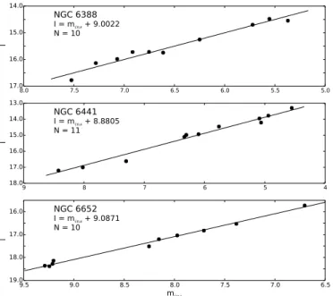
(4) A&A 573, A103 (2015) Table 3. Format for the time-series photometry of all confirmed variables in our field of view of the five clusters. Cluster. #. Filter. NGC 6388 NGC 6388 .. . NGC 6441 NGC 6441 .. .. V29 V29 .. . V63 V63 .. .. I I .. . I I .. .. HJD (d) 2 456 436.95140 2 456 455.86035 .. . 2 456 454.78961 2 456 509.61751 .. .. Mstd (mag) 14.620 14.375 .. . 16.770 16.561 .. .. σm fref σref fdiff σdiff (mag) (ADU s−1 ) (ADU s−1 ) (ADU s−1 ) (ADU s−1 ) 0.003 44 901.760 4397.950 54 393.674 627.525 0.003 44 901.760 4397.950 87 182.547 578.940 .. .. .. .. .. . . . . . 0.007 9899.919 2247.418 –17 795.506 260.090 0.005 9899.919 2247.418 –8594.633 212.423 .. .. .. .. .. . . . . .. mins (mag) 5.617 5.372 .. . 7.889 7.680 .. .. p 4.6389 3.3446 .. . 6.1094 6.0163 .. .. Notes. The standard Mstd and instrumental mins magnitudes listed in Cols. 5 and 6 respectively correspond to the cluster, variable star, filter and epoch of mid-exposure listed in Cols. 1–4, respectively. The uncertainty on mins is listed in Col. 7, which also corresponds to the uncertainty on Mstd . For completeness, we also list the reference flux fref and the differential flux fdiff (Cols. 8 and 10 respectively), along with their uncertainties (Cols. 9 and 11), as well as the photometric scale factor p. Instrumental magnitudes are related to the other quantities via mins = 17.5−2.5·log10 ( fref + fdiff /p). This is a representative extract from the full table, which is available at the CDS. 14.0. I = mins + 9.0022 N = 10. I. 15.0. where mins is the instrumental magnitude, to provide approximate I magnitudes for these two clusters as well.. NGC 6388. 16.0 17.08.0 13.0 14.0. 7.5. 7.0. 6.5. 6.0. 5.5. 5.0. NGC 6441. I = mins + 8.8805 N = 11. I. 15.0. 2.6. Colour–magnitude diagrams. 16.0 17.0 18.09. I. 16.0 17.0. 8. 7. 6. 5. 4. NGC 6652. I = mins + 9.0871 N = 10. 18.0 19.09.5. 9.0. 8.5. 8.0. mins. 7.5. 7.0. 6.5. Fig. 1. Standard I magnitudes against the instrumental magnitudes. The solid line in each panel shows the best fit calibration.. 2.5. Photometric calibration. Using the colour information that is available from the colour– magnitude diagram (CMD) data (see Sect. 2.6), rough photometric calibrations can be made for NGC 6388, NGC 6441 and NGC 6652. A number of reasonably isolated stars were selected and by matching their positions with the CMD data, their standard I magnitudes were retrieved. By finding the offset between the standard I magnitudes and the mean instrumental magnitudes found by DanDIA, a rough photometric calibration was found. Figure 1 shows a plot of the standard I magnitudes versus the mean instrumental magnitudes along with the fit for each of the clusters where CMD data are available. Due to the non-standard filter that is used for these observations, the photometric calibration is only approximate and there is therefore some added uncertainty in the listed I magnitudes. For NGC 6528 and NGC 6638 where no CMD data are available, we have chosen to adopt the photometric conversion of I = mins + 9.0, A103, page 4 of 23. (5). As we only have observations in one filter, it is not possible to make a CMD based on our own data. Three of the clusters; NGC 6388, NGC 6441 and NGC 6652; are part of The ACS Survey of Galactic Globular Clusters (Sarajedini et al. 2007), and the data files from the survey, that include V and I magnitudes and celestial coordinates, are available online2 . We were able to match many of the variable stars using celestial coordinates and I magnitudes, enabling us to recover colour information for these objects. Unfortunately, for some of the variables, their proximity to a bright star meant that we were unable to do this. For NGC 6528 and NGC 6638, no suitable data to create a CMD were found. The Piotto et al. (2002) study includes NGC 6638, but the data files that are available do not contain any celestial coordinates and are therefore not useful for our purposes.. 3. Results Several methods were used to detect the variable stars in our data. Firstly an image representing the sum of the absolutevalued difference images with pixel values in units of sigma, was constructed for each cluster. These images were visually inspected for peaks indicating stars that show signs of variability. Secondly a diagram of the root-mean-square (rms) magnitude deviation versus mean magnitude for the calibrated light curves was produced, from which we selected stars with a high rms for further inspection. Finally, the difference images were blinked in sequence in order to confirm the variations of all suspected variables. Period estimates were made using a combination of the string-length statistic S Q (Dworetsky 1983) and the phase dispersion minimisation method (Stellingwerf 1978). The results for each cluster are presented below. Note that the RR Lyrae (RRL) nomenclature introduced by Alcock et al. (2000) has been adopted for this paper; thus RR0 designates an RRL pulsating in the fundamental mode, RR1 designates an RRL pulsating in the first-overtone mode, and RR01 designates a double-mode (fundamental and first-overtone) RRL. 2. http://www.astro.ufl.edu/~ata/public_hstgc/.
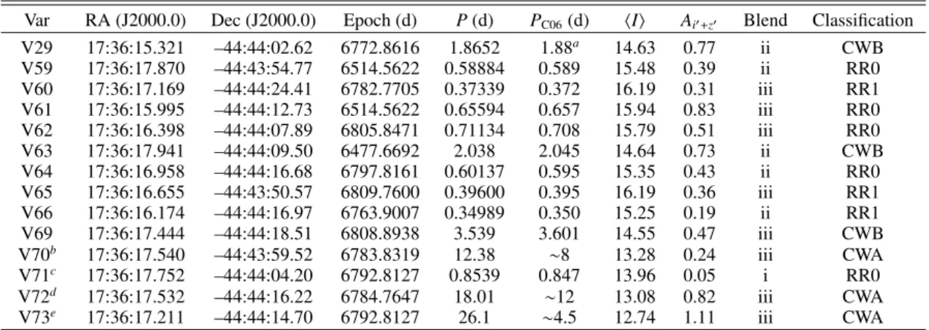
(5) J. Skottfelt et al.: Variable stars in metal-rich globular clusters. Stars in the upper part of the instability strip are in some parts of the literature referred to as Population II Cepheids (P2C). We have adopted the “W Virginis” or “CW” nomenclature, with sub-classifications CWA for CW stars with periods between 8 and 30 days, and CWB for CW stars with periods shorter than 8 days (General Catalog of Variable Stars (GCVS), Samus et al. 2009). CW stars with periods between 0.8 and 3 days are possibly anomalous Cepheids (AC), which are believed to be too luminous for their periods. If the period is longer than 30 days, then we classify them as RV Tauri stars (RV; Clement et al. 2001). For variable stars on the red giant branch (RGB), which in some parts of the literature are just referred to as long period variables (LPV), we have adopted the nomenclature of the GCVS. Thus stars on the RGB showing a noticeable periodicity and with periods over 20 days are classified as semiregular (SR), and stars that show no evidence of periodicity are classified as long-period irregular (L). Note that some stars might actually be on the asymptotic giant branch (AGB) and not the RGB. However, distinguishing the two is difficult without a proper spectroscopic analysis and is therefore not possible from the CMDs in this study. 3.1. NGC 6388 3.1.1. Background information. The first 9 variable stars in NGC 6388 were reported by Lloyd Evans & Menzies (1973). These were assigned the numbers V1-V9 by Sawyer Hogg (1973) in her third catalogue of variable stars in globular clusters. Three new variables, V10-V12, were found by Lloyd Evans & Menzies (1977) using observations from V and I band photographic plates. They also confirmed the existence of the previous 9 variables, but were not able to provide periods for any of the variables. Using B-band photographic plate observations, Hazen & Hesser (1986) presented 14 new variables, V13-V26, within the tidal radius, and 4 field variables. Silbermann et al. (1994) were the first to use CCD observations to search for variable stars in the cluster, and were able to find 3 new variables, V27-V29, and 4 suspected ones. Periods were given for the three new variables and for V17 and V20. From observations obtained at the 0.9 m telescope at the Cerro Tololo Inter-American Observatory (CTIO), Pritzl et al. 2002, hereafter P02) were able to find 28 new variables, V30-V57, which includes 3 of the 4 suspected variables in Silbermann et al. (1994). The data for the P02 paper were obtained over 10 days, so only very few long period variables were found. Due to the high central concentration (see Table 1) none of the variable stars found up to this point are located in the central part of the cluster, except for V29. However, when the P02 data were re-analysed by Corwin et al. (2006, hereafter C06) using the ISIS version 2.1 image-subtraction package (Alard 2000; Alard & Lupton 1998), 12 new variables, V58-V69, and 6 suspected ones, denoted SV1-SV6, were found. All of these variables are either RRL or CW stars and most of them are located in the central parts of the cluster. 3.1.2. This study. A finding chart for the cluster containing the variables detected in this study is shown in Figs. 2 and 3 shows a CMD of the stars in our FoV, with the variables overplotted.. Figure 4 shows the rms magnitude deviation for the 1824 stars with calibrated I light curves versus their mean magnitude. From this plot it is evident that stars fainter than 18th magnitude have not been detected, which can probably be explained by the very dense stellar population in the central region of the cluster. This creates a very high background intensity, which makes it hard to detect faint stars, and which increases the possibility of blending, making some stars appear brighter than they are. 3.1.3. Known variables. All of the previously known variables within our FoV are recovered in this analysis. The light curves for these variables are shown in Fig. 5 and their celestial coordinates and estimated periods are listed in Table 4, along with the periods found in C06. The table also reports the mean I magnitude, the amplitude in our filter, and the classification of the variables. A discussion of individual variables is given below, but generally it can be noted that we find similar periods to those given in C06. Only the three CWs; V70, V72 and V73; have very different periods. In C06 these three stars are listed as suspected variables (SV) due to uncertainty in the classification. We find some variables to be somewhat brighter than would be expected for their classification. This is most likely due to blending with very close neighbours which, as mentioned above, can lead to an overestimation of the reference flux (e.g. see Col. 9 of Table 4). An overestimated reference flux subsequently leads to an underestimation of the amplitude of the variable star. Errors in the mean magnitudes might also be caused by the rough photometric calibration, but this should only give discrepancies on a much lower level, and should not affect the amplitude. Unless otherwise stated below, the classifications that are given in P02 or C06 are confirmed by our light curves and the CMD, and have therefore been adopted. A period-luminosity diagram for the stars in the upper part of the instability strip is shown in Fig. 22, and is discussed in more detail in Sect. 4.1. Discussion of individual variables (square brackets gives approximate position in the CMD as [V − I, V]): V29, V63: based on the relation between period and luminosity compared to the other CW stars, these two stars are classified as CWB stars and not AC stars. V29 is the only variable that is also found in the P02 paper, i.e. where difference image analysis was not used. V59, V60: no matching stars have been found in the CMD for these two variables. However, their periods, mean magnitude, and amplitude strongly indicate that the classifications as RR0 and RR1, respectively, are correct. V61-V62, V64-V65: CMD positions, periods, magnitudes and amplitudes all verify the classifications given in C06. V66: this RR1 seems to have an overestimated mean magnitude, and correspondingly underestimated amplitude. This is most likely caused by blending with another star, as the position in the CMD [0.4, 16.5] verifies the classification. V69: no CMD position for this star is found, but based on its period and mean magnitude it is classified as a CWB. V70, V73: those are two of the suspected variables from C06 that are also in our FoV. We report reliable periods in Table 4. The periods and CMD positions ([1.0, 14.3], [1.0, 13.6]) indicate that they are CWA stars. V71: this star is also a suspected variable from C06. The star is highly blended with a brighter star which leads to a mean magnitude that is too bright and a heavily underestimated A103, page 5 of 23.
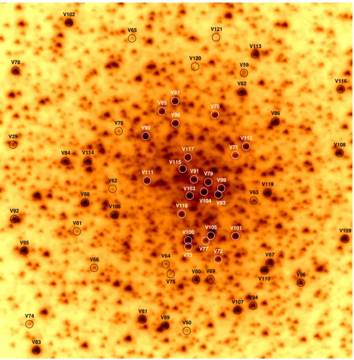
(6) A&A 573, A103 (2015). V102 V121. V65. V113 V120 V78. V59 V116. V82 V97 V85. V70 V86. V98 V76 V90 V29. V112 V117. V114. V84. V108. V71. V115 V91 V79. V111. V99. V62. V119 V103. V63. V88 V104. V93. V118. V106 V92 V61. V105. V101. V109. V100 V95 V77 V64. V66. V72. V87. V73 V80. V69. V96 V110. V75 V94 V107 V81 V74. V89 V60. V83. Fig. 2. NGC 6388: finding chart constructed from the reference image marking the positions of the variable stars. Labels and circles are white/black only for clarity. North is up and east is to the right. The cluster image is ∼4100 by 4100 .. amplitude. No CMD position is available, but its period and light curve strongly suggest that the star is an RR0. V72: this is the last of the C06 suspected variables in our FoV, and we report a reliable period in Table 4. No CMD position is found for this variable, so it could be a SR, but CWA is a more likely classification considering the relationship between magnitude and period compared to the other CW stars (see Fig. 22).. 3.1.4. New variables. In this study we were able to find 48 new variable stars for NGC 6388. Their light curves are shown in Fig. 6 and their details are listed in Table 5. A103, page 6 of 23. Most of the new variables are RGB stars and many of them have small amplitudes, which is probably the reason why they have not been detected until now. There are however also two (possibly three) previously undetected RRL stars and three new CW stars. For many of the new long period variables it has been hard to determine a period, which may indicate that they are irregular. Discussion of individual variables: V74: this star has a very noisy light curve, where a period matching an RR1 has been estimated. The mean magnitude also matches this classification, but it falls on the red-clump in the CMD [1.0, 16.9]. Our RR1 classification is therefore tentative. V75: the light curve and the position of the star in the CMD [0.5, 16.7], strongly suggest that this is an RR1..
(7) J. Skottfelt et al.: Variable stars in metal-rich globular clusters 12 13 14. V. 15 16 17 18 19 20 0.0. 0.5. 1.0. 1.5. 2.0. V-I. 2.5. 3.0. Fig. 3. NGC 6388: (V − I), V colour–magnitude diagram made from HST/ACS data as explained in Sect. 2.6. The stars that show variability in our study are plotted as follows: RRL as filled circles (RR0 in red, RR1 in green, RR01 in blue), CW as filled triangles (CWA in green, CWB in cyan, AC in magenta, RV in yellow), and RGB stars as filled squares (SR in red, L in blue). An open symbol means that the classification is uncertain.. 1. SR stars. Most of the stars have fairly small amplitudes (0.04–0.15 mag) V92, V93: these two stars are not in the CMD, but based on their periods and luminosity they are most likely SR stars. V96-V118: These stars are also on the RGB, but it has not been possible to find any periods that phase their light curves satisfactorily. We have therefore classified them as L stars. V119: the position of this star in the CMD [0.8, 13.4] puts it in the CW region. However, we have not been able to find a period that phases the light curve properly and the star has therefore been tentatively classified as an L star. V120, V121: these two stars were not identified by the pipeline and no stars are visible at these positions on the reference image. However, when blinking the difference images some variability is clearly seen and the differential fluxes have thus been measured for these positions in the difference images. This means that there is no measurement of the reference flux and magnitudes or amplitudes are therefore not given. The fact that the stars are not visible on the reference image is probably because they are very faint at the epoch of the reference image. No good candidates for the stars have been found in the CMD, and no reasonable periods could be estimated. Without more information it is hard to classify the two stars, but one possibility could be a type of cataclysmic variable, as these are known to have prolonged low and high states, which can be quasi-periodic or have no clear periodicity.. RMS (mag). 3.2. NGC 6441 3.2.1. Background information. 0.1. 0.01. 0.001 11. 12. 13. 14. 15. Mean I magnitude. 16. 17. 18. Fig. 4. NGC 6388: plot of the rms magnitude deviation versus the mean magnitude for each of the 1824 calibrated I light curves. The variables are plotted with the same symbols as in Fig. 3.. V76: this star has a very good light curve, where the light curve shape, period and mean magnitude strongly indicate an RR0. However, the CMD position [1.1, 16.8] is a little discrepant. V77: no CMD information is available for this star, but as the luminosity seems a bit too high compared to its period, we classify it as a possible AC (see Fig. 22). The star is located very close to another and much brighter variable V105, and it would have been very difficult to resolve these stars using conventional imaging. V78, V79, V81: these three stars have similar positions in the CMD [1.7, 14], and they are therefore most likely SR stars. V80,V82: these two stars are most likely RV stars, based on their position in the CMD [1.1, 12.8] and their relation between period and luminosity (see Fig. 22). V83-V92,V94,V95: all of these stars are on the RGB and combined with their long periods, these can be classified as. The first 10 variables in NGC 6441 were found by Fourcade et al. (1964). In Hesser & Hartwick (1976) the authors report that they may have found two variable stars. These two stars are, however, found to be non-variable in Layden et al. (1999), whom made use of CCD imaging. Layden et al. (1999) were able to identify, classify, and determine periods for 31 long period variables, 11 RRL stars and 4 eclipsing binaries. A further 9 suspected variables were found but not classified. From CTIO observations, Pritzl et al. (2001) were able to find 48 new variables, of which 35 are RRL stars. Similar to NGC 6388, this cluster has a high central concentration (see Table 1), and none of the variable stars found up to this point are located in the central part of the cluster, except for V63. Pritzl et al. (2003, hereafter P03) used HST observations to reveal 41 previously undiscovered variables, V105–V145, the main part of which are located in the central parts. The Pritzl et al. (2001) data were also re-analysed using ISIS in the C06 paper. In this analysis, five new variables, V146-V150, were found (and recovered in the HST data), but three variables (V136, V138, and V145) that were found in the HST data were not found in the ISIS analysis – all three bonafide variables located within 1000 of the centre of the cluster. 3.2.2. This study. A finding chart for the cluster containing the variables detected in this study is shown in Figs. 7, and 8 shows a CMD of the stars within our FoV, with the variables overplotted. Figure 9 shows the rms magnitude deviation for the 1860 stars with calibrated I magnitudes versus their mean magnitude. From this plot it is evident that stars fainter than 18th magnitude have not been detected, which can probably be A103, page 7 of 23.
(8) A&A 573, A103 (2015). 0.0. I I. 0.5. 1.0. 0.5. 1.0. V64 P=0.60137. 0.5. 1.0. V70 P=12.38. 13.15. 13.92. 0.0. 0.5. 1.0. V71 P=0.8539. 13.94. 13.25. 0.5. 1.0. 16.4. 0.5. 1.0. 0.0. 0.5. 1.0. V66 P=0.34989. 16.1 14.2. 0.0. 0.5. 1.0. V69 P=3.539. 14.4 15.25. 14.6. 15.35 0.0. 0.5. 1.0. 0.0 12.0. V72 P=18.01. 0.5. 1.0. 14.8. 0.0. 0.5. 1.0. V73 P=26.1. 12.4 12.8. 13.4 0.0. 15.9. 15.15. 13.0. 13.98 0.0. V65 P=0.39600. 12.6. 13.96. 13.35. 1.0. 16.2. 15.5 0.0. 0.5. 16.0. 15.3. 14.6. 0.0. V62 P=0.71134. 15.5 15.7. 16.2. 16.4 0.0. V61 P=0.65594. 15.8. 16.2. 15.1. V63 P=2.038. 15.4. V60 P=0.37339. 16.0. 15.6. 14.2. 15.0. V59 P=0.58884. 15.4. 14.6 15.0. I. 15.2. V29 P=1.8652. 14.2. 13.2 0.0. 0.5. 1.0. 0.0. 0.5. 1.0. Fig. 5. NGC 6388: phased light curves for the known variables in our FoV. Red triangles are 2013 data and blue circles are 2014 data. Error bars are plotted but are smaller than the data symbols in many cases. Table 4. NGC 6388: details of the 14 previously known variables in our FoV. Var V29 V59 V60 V61 V62 V63 V64 V65 V66 V69 V70b V71c V72d V73e. RA (J2000.0) 17:36:15.321 17:36:17.870 17:36:17.169 17:36:15.995 17:36:16.398 17:36:17.941 17:36:16.958 17:36:16.655 17:36:16.174 17:36:17.444 17:36:17.540 17:36:17.752 17:36:17.532 17:36:17.211. Dec (J2000.0) –44:44:02.62 –44:43:54.77 –44:44:24.41 –44:44:12.73 –44:44:07.89 –44:44:09.50 –44:44:16.68 –44:43:50.57 –44:44:16.97 –44:44:18.51 –44:43:59.52 –44:44:04.20 –44:44:16.22 –44:44:14.70. Epoch (d) 6772.8616 6514.5622 6782.7705 6514.5622 6805.8471 6477.6692 6797.8161 6809.7600 6763.9007 6808.8938 6783.8319 6792.8127 6784.7647 6792.8127. P (d) 1.8652 0.58884 0.37339 0.65594 0.71134 2.038 0.60137 0.39600 0.34989 3.539 12.38 0.8539 18.01 26.1. PC06 (d) 1.88a 0.589 0.372 0.657 0.708 2.045 0.595 0.395 0.350 3.601 ∼8 0.847 ∼12 ∼4.5. hIi 14.63 15.48 16.19 15.94 15.79 14.64 15.35 16.19 15.25 14.55 13.28 13.96 13.08 12.74. Ai0 +z0 0.77 0.39 0.31 0.83 0.51 0.73 0.43 0.36 0.19 0.47 0.24 0.05 0.82 1.11. Blend ii ii iii iii iii ii ii iii ii iii iii i iii iii. Classification CWB RR0 RR1 RR0 RR0 CWB RR0 RR1 RR1 CWB CWA RR0 CWA CWA. Notes. The celestial coordinates correspond to the epoch of the reference image, which is the HJD ∼ 2 456 522.48 d. Epochs are (HJD – 2 450 000). hIi denotes mean I magnitude and Ai0 +z0 are the amplitudes found in our special i0 + z0 filter. The blend column describes whether the star is blended with (i) brighter star(s); (ii) star(s) of similar magnitude; or (iii) fainter/no star(s). PC06 are periods from C06, which have been included as a reference. (a) Period from Pritzl et al. (2002). (b) Denoted SV1, (c) SV2, (d) SV4, and (e) SV5 in C06.. explained by the very dense stellar population in the central region, similar to NGC 6388. 3.2.3. Known variables. All of the previously known variables within our FoV are recovered in this analysis. The light curves for these variables are shown in Fig. 10, and their details are listed in Table 6. The table includes the periods found in P03 and C06. A discussion of individual variables is given below, but generally it can be noted that for all RRL and CW variables, the same periods are estimated as in P03 and/or C06. For the long period variables there are a few discrepancies. A number of the variables are found to be somewhat brighter than in P03. This is most likely due to blending with very close neighbours, leading to an overestimation of the reference flux. The classification that is given in P03 and/or C06 seems to be correct in almost all cases and have thus been adopted, unless otherwise noted below. A period-luminosity diagram for the stars in the upper part of the instability strip is shown in Fig. 22, and is discussed in more detail in Sect. 4.1. A103, page 8 of 23. Satisfactory light curves are found for the three variables that were not detected by C06: V136, V138, and V145. Of the five new variables that C06 discovered, three (V146-V148) are within our FoV and have reasonable light curves. This highlights the power of EMCCD observations and DIA combined. Discussion of individual variables: V63: this RR0 is the only variable that is also found in Pritzl et al. (2001). V105: we find a slightly shorter period for this SR than in P03. V110, V122: no CMD positions are found for these two variables, but their periods and phased light curves clearly indicate that they are RR0 stars. V111: this RR0 is highly blended with a brighter star, and the mean magnitude is therefore too bright. Due to the strong blending the correct position in the CMD has not been found. V113, V121: due to blending with nearby stars of similar brightness, these RR0 stars have overestimated mean magnitudes. V114: this RR0 star is heavily blended with a brighter star. V117, V119: both stars are in a very crowded area and their positions and reference fluxes were not found by the pipeline. The correct positions of the stars were found in the summed difference image, and the differential fluxes have.
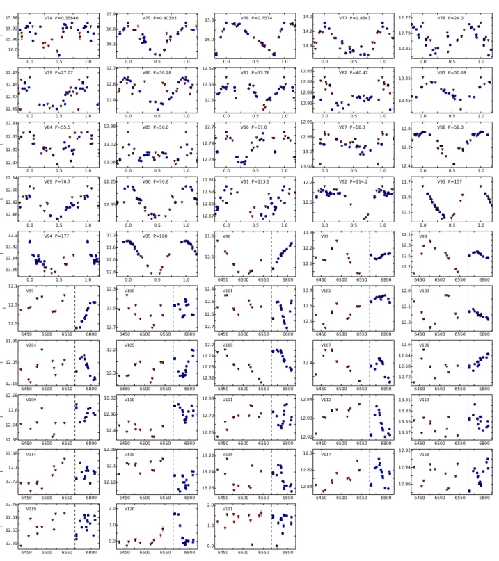
(9) J. Skottfelt et al.: Variable stars in metal-rich globular clusters 15.88. 15.9. V74 P=0.35840. I. 15.92. V75 P=0.40393. 14.0. V76 P=0.7574. 15.6. 16.0. 15.96. 14.2 16.0. 16.1. 16.0 0.0 12.43. 0.5. 1.0. V79 P=27.07. 12.7. 0.0. 0.5. 1.0. V80 P=30.28. 12.8. 12.52. 0.0. 0.5. 1.0. 12.47 12.49 12.81. 0.0. 0.5. 1.0. I. 12.83 12.85 12.87 12.34. 0.0. 0.5. 0.0. 1.0. 13.06. 12.78 0.0. 12.25. 0.5. 1.0. V90 P=70.8. I. 12.46. I. 13.3. 0.5. 1.0 11.2. V94 P=177. 13.32. 11.6. 13.34. 12.0. 13.36. 12.4. I. 0.0. 0.5. 1.0. 12.3. V99. 12.3. 0.5. 0.0. 0.5. 1.0. 6450. 6500. 6550. 6800. V104. 12.7 12.2. 6450. 6500. 6550. 6800. I. 12.6. 6450. 6500. 6550. 6800. V114. 6450. 6500. 6550. 6800. 12.2. V105. 1.0. 6550. 6800. 6450. 6500. 6550. 6800. V115. 6500. 6550. 6800. 6450 2.0. V119. 6500. 6550. 6800. V120. 1.0. 12.53. 13.02. 0.0. 0.5. 1.0. V92 P=114.2. 6450. 6500. 6550. 6800. 12.4. 0.0. 0.5. 1.0. V93 P=157. 11.7 11.9. 6550. 11.8. 0.0. 0.5. 1.0. 12.2. 12.3. 12.6. 12.7. 6800. 6450 12.4. 6500. 6550. 6800. 6550. 6800. 1.0. 6500. 6550. 6800. 6500. 6550. 6800. 6500. 6550. 6800. 6500. 6550. 6800. 6500. 6550. 6800. V103. 12.1 12.2 6450. V106. 6450 12.0. V102. 12.5. 6500. 0.5. V98. 12.5. 12.6 6450. 0.0 12.1. V97. 6500. 6550. 6800. 6450 12.6. V107. V108. 12.64. 12.4. 12.68 12.72. 6500. 6550. 6800. 6450 12.84. V111. 6500. 6550. 6800. 6550. 6800. 12.92 12.8. V116. 13.35 13.37 6450. 6500. 6550. 6800. V117. 12.92. 12.82. 12.94. 13.26. 12.84. 12.96. 6450. 6500. 6550. 6800. 6500. 6550. 6800. V113. 13.33. 12.88. 6500. 6450 13.31. V112. 13.24. 2.0. 1.0. 6450. 6500. 6550. 6800. 6450 V118. 6450. V121. 1.0. 0.0. 12.55. 6500. V101. 6450 13.22. I. 12.12. V96. 6450 12.68. V110. 0.5 V88 P=58.3. 12.2. 12.32. 12.76. 12.08. 1.0. 12.28 6500. 0.0 12.0. 12.1 0.5. 12.24. 12.4. 12.72 6450. 12.7. 12.72. 12.1. 12.51 I. 0.5 V87 P=58.3. 12.6. 12.5. 12.36. 12.7. 12.49. 0.0. 12.2. 12.6. 6450 12.32. V109. 12.64. 12.68. 1.0. V91 P=113.9. 6450 12.4. V100. 12.3. 12.68. 0.5. 12.5. 12.05. 12.56. 12.96. 13.0. 0.0 11.5. V95 P=180. 1.0. 12.98. 0.0. 1.0. 12.5. 12.5. I. 0.0. 0.5 V83 P=50.68. 12.45. 12.67 0.0. 12.15. 1.0. 12.65. 12.35. 0.0 12.35. 12.63. 12.42. 11.95. 0.5 V86 P=57.0. 12.61. 12.38. 12.1. 0.0. 12.74. V82 P=40.47. 12.91. 12.7. 13.02. 1.0. V89 P=70.7. 0.5 V85 P=56.8. 1.0. 12.89. 12.6. 12.98. V84 P=55.5. 0.5. 12.87. 12.56. 12.9. 12.81 0.0. 12.85. V81 P=33.78. V78 P=24.0. 12.79. 14.4. I. 12.45. 12.77. V77 P=1.8643. 6450. 6500. 6550. 6800. 0.0. 6450. Fig. 6. NGC 6388: light curves for the new variables in our FoV. Red triangles are 2013 data and blue circles are 2014 data. Error bars are plotted but are smaller than the data symbols in many cases. Light curves with confirmed periods are phased. For those variables without periods the x-axis refers to (HJD – 2 450 000), and the dashed line indicates that the period from HJD 2 456 570 to 2 456 760 has been removed from the plot, as no observations were performed during this time range. Note that V120 and V121 are plotted in differential flux units, 103 ADU/s, and not calibrated I magnitudes.. been measured for these positions in the difference images. Therefore, as no reference flux could be measured, magnitudes and amplitudes are not given for either of these RR0 stars. V118: using the period of this star, P03 and C06 can not give a certain classification, but suggest RR0 or CW. Based on the position of the star in the CMD [0.82, 16.9] we classify it as an RR0 star, although the period is unusually long for this type of star.. V120: this variable is classified as an RR1 in both P03 and C06. Due to the scatter in our light curve and the position of the star in the CMD [0.60, 17.3], we have analysed the light curve for any secondary periods, but none have been found. We therefore support the RR1 classification. V126-V129: in P03 these stars are described as CWA candidates. The positions that these stars occupy in the CMD [(1.0−1.3), (14.0−15.5)], seem to support that they are indeed CWA stars. A103, page 9 of 23.
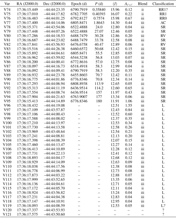
(10) A&A 573, A103 (2015) Table 5. NGC 6388: Details of the 48 new variables found in the cluster. Var V74 V75 V76 V77 V78 V79 V80 V81 V82 V83 V84 V85 V86 V87 V88 V89 V90 V91 V92 V93 V94 V95 V96 V97 V98 V99 V100 V101 V102 V103 V104 V105 V106 V107 V108 V109 V110 V111 V112 V113 V114 V115 V116 V117 V118 V119 V120 V121. RA (J2000.0) 17:36:15.449 17:36:17.010 17:36:16.483 17:36:17.400 17:36:15.371 17:36:17.448 17:36:17.286 17:36:16.687 17:36:17.841 17:36:15.516 17:36:15.892 17:36:16.962 17:36:18.200 17:36:18.097 17:36:16.092 17:36:16.932 17:36:16.775 17:36:17.293 17:36:15.313 17:36:17.554 17:36:17.904 17:36:15.413 17:36:18.432 17:36:17.109 17:36:17.106 17:36:17.588 17:36:17.210 17:36:17.730 17:36:15.969 17:36:17.241 17:36:17.398 17:36:17.460 17:36:16.413 17:36:17.731 17:36:18.893 17:36:18.929 17:36:18.038 17:36:16.778 17:36:17.873 17:36:17.999 17:36:16.136 17:36:17.172 17:36:18.924 17:36:17.231 17:36:17.147 17:36:18.093 17:36:17.337 17:36:17.575. Dec (J2000.0) –44:44:23.35 –44:44:17.82 –44:44:01.25 –44:44:14.06 –44:43:54.06 –44:44:07.26 –44:44:18.53 –44:44:23.02 –44:43:56.93 –44:44:26.38 –44:44:04.61 –44:43:59.02 –44:44:00.41 –44:44:16.73 –44:44:09.41 –44:44:23.78 –44:44:01.86 –44:44:06.94 –44:44:11.19 –44:44:08.74 –44:44:21.63 –44:44:14.89 –44:44:19.08 –44:43:57.87 –44:44:00.43 –44:44:08.02 –44:44:13.97 –44:44:13.58 –44:43:48.64 –44:44:08.81 –44:44:08.39 –44:44:13.47 –44:44:10.89 –44:44:22.13 –44:44:04.17 –44:44:14.09 –44:44:17.56 –44:44:06.99 –44:44:03.22 –44:43:52.65 –44:44:04.61 –44:44:05.70 –44:43:56.82 –44:44:04.38 –44:44:10.91 –44:44:08.59 –44:43:53.93 –44:43:50.60. Epoch (d) 6790.7919 6782.7705 6792.8127 6805.8471 6522.4888 6522.4888 6488.7479 6488.7479 6476.6758 6460.6572 6805.8471 6544.5238 6772.8616 6518.4918 6790.7919 6455.8603 6776.8346 6808.8938 6436.9514 6436.9514 6763.9007 6776.8346 – – – – – – – – – – – – – – – – – – – – – – – – – –. P (d) 0.35840 0.40393 0.7574 1.8643 24.0 27.07 30.28 33.78 40.47 50.68 55.5 56.8 57.0 58.3 58.3 70.7 70.8 113.9 114.2 157 177 180 – – – – – – – – – – – – – – – – – – – – – – – – – –. hIi 15.96 16.07 15.98 14.30 12.80 12.46 12.86 12.58 12.89 12.42 12.85 13.03 12.75 12.99 12.20 12.42 12.34 12.65 12.60 11.97 13.34 11.91 12.51 12.43 12.52 12.37 12.53 12.58 12.54 12.13 12.07 12.27 12.28 12.41 12.68 12.63 12.38 12.73 12.88 13.35 12.71 12.11 13.24 12.83 12.95 12.53 – –. Ai0 +z0 0.12 0.22 0.67 0.44 0.04 0.05 0.20 0.08 0.06 0.15 0.05 0.07 0.08 0.04 0.35 0.11 0.14 0.05 0.65 0.43 0.06 1.06 1.55 0.84 0.60 0.35 0.34 0.26 0.21 0.20 0.15 0.14 0.12 0.12 0.12 0.09 0.08 0.08 0.07 0.06 0.05 0.04 0.04 0.04 0.04 0.05 – –. Blend ii ii iii iii iii ii iii iii ii iii iii iii ii ii iii iii ii iii ii iii iii iii iii iii iii iii ii iii iii iii iii ii iii iii iii iii iii iii iii iii iii ii iii iii iii iii – –. Classification RR1? RR1 RR0 AC SR SR RV SR RV SR SR SR SR SR SR SR SR SR SR SR SR SR L L L L L L L L L L L L L L L L L L L L L L L L? ? ?. Notes. The celestial coordinates correspond to the epoch of the reference image, which is the HJD ∼ 2 456 522.48 d. Epochs are (HJD – 2 450 000). hIi denotes mean I magnitude and Ai0 +z0 are the amplitudes found in our special i0 + z0 filter. The blend column describes whether the star is blended with (i) brighter star(s); (ii) star(s) of similar magnitude; or (iii) fainter/no star(s).. V130: the period of P03 does not phase our light curve well and our best fit period is significantly longer. Some of the data points seem to have a sort of systematic scatter and it may therefore be an L star, which is supported by its position in the CMD, [1.64, 15.0]. V132: this star is quite heavily blended, which is reflected in a rather scattered light curve and the fact that we found a mean I magnitude that is about a magnitude higher than what was found in P03. Based on its position in the CMD and the relation between period and luminosity, we classify this star as a CWB. A103, page 10 of 23. V133, V137: for these two stars it is not possible to phase the light curves properly with the periods given in P03, or any other period, and this suggests that they are L stars. No period is therefore given for these two variables. V136, V138: these two RR0 stars were not found in the C06 analysis. Our data are properly phased by the periods of P03. V139: this SR phases well with the period found by P03. V144: the period from P03 does phase this SR reasonably well, but the phased light curve still looks a bit peculiar, so it might also be an L star..
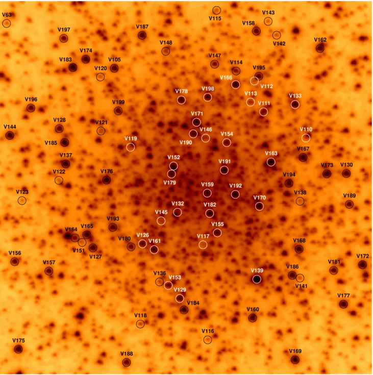
(11) J. Skottfelt et al.: Variable stars in metal-rich globular clusters V143. V63. V115 V158. V187. V197. V148. V162. V142. V174 V183. V147. V105. V114 V195. V120 V166. V196. V112. V198. V178. V113. V199. V133 V111. V171 V128. V121. V144. V110. V146 V154 V119. V190. V185. V167 V137. V163. V152 V191. V173. V176. V122. V130. V194 V179. V159. V192. V123. V138. V189. V170 V132. V182. V145 V193 V164. V155. V165 V180. V126 V161. V117 V168. V151. V156. V172. V127 V181. V157 V139. V136. V186. V153 V141. V129. V177 V184 V160 V118 V116 V175 V169. V188. Fig. 7. NGC 6441: finding chart constructed from the reference image marking the positions of the variable stars. Labels and circles are white/black only for clarity. North is up and east is to the right. The cluster image is ∼4100 by 4100 .. V145: this star is highly blended with a star of similar brightness and was not found in the C06 paper. P03 classifies this as an RR1. We are able to find a fundamental and first overtone period of P0 = 0.72082 and P1 = 0.55588, respectively. This gives a first-overtone to fundamental period ratio of P1 /P0 = 0.7712, which is only slightly higher than the “canonical” ratio of ∼0.745 (Clement et al. 2001). We therefore classify this as a double-mode RRL, which also agrees well with the position of the star in the CMD [0.64, 17.3]. Studies of other clusters and dwarf galaxies have shown that the period ratio for RR01 stars generally does not exceed 0.748 (e.g. Clementini et al. 2004, figure 13), and the period ratio for this star should therefore be confirmed when more data become available for NGC 6441.. V146-V148: these RR1 stars seems to be blended with multiple stars. However, their periods and light curves, although with some scatter, are consistent with their classification. 3.2.4. New variables. In this study we were able to find 49 new variable stars for NGC 6441. These are all listed in Table 7 and their light curves are shown in Fig. 11. Similar to NGC 6388, most of the new variables are RGB stars, many with small amplitudes, which is probably the reason why they have not been detected until now. There are, however, also one (possibly two) previously undetected A103, page 11 of 23.
(12) A&A 573, A103 (2015) 12 13 14. V. 15 16 17 18 19 20 0.0. 0.5. 1.0. 1.5. 2.0. V-I. 2.5. 3.0. Fig. 8. NGC 6441: (V − I), V colour–magnitude diagram made from HST/ACS data as explained in Sect. 2.6. The stars that show variability in our study are plotted with the same symbols as in Fig. 3.. RMS (mag). 1. positions and differential fluxes were found manually, but again the reference flux is not measured, so no magnitude or amplitude is given. Based on the period, light curve shape, and CMD position [0.85, 17.4], we classify this tentatively as an RR0 star. V153, V154: based on their periods, light curves, and positions in the CMD [1.05, 15.0], we classify these two stars as CWA stars. V155: both the period and magnitude suggest that this is either a CW or an SR star, but the position of this star in the CMD is [−0.5, 13.5], which means that it is far too blue to fit any of these classifications. We do not attempt to classify this variable. V156-V162, V165-V168: the CMD puts all of these stars on the RGB. As it has been possible to estimate periods for them, we classify these as SR stars. V163: this star has no CMD information, but based on the period, light curve, and magnitude, it is most likely an SR star. V164: the CMD position [1.1, 15.5] and the mean magnitude of this star would normally imply that it is a CW star. However the light curve is scattered and the derived period uncertain. We refrain from classifying this variable. V169-V199: we have classified these RGB stars for which we have been unable to derive periods as L stars. 3.3. NGC 6528. 0.1. 3.3.1. Background information. 0.01. 0.001 11. 12. 13. 14. 15. Mean I magnitude. 16. 17. 18. Fig. 9. NGC 6441: plot of the rms magnitude deviation versus the mean magnitude for each of the 1860 calibrated I light curves. The variables are plotted with the same symbols as in Fig. 3.. RRL stars and two new CW stars. For many of the new long period variables it has been hard to determine a period, which could indicate that they are irregular. It should be noted that three of the new variables (V151, V164, and V165) are located very close to each other. Resolving these three variables would have been difficult using conventional imaging, as they are all within a radius of ∼0.00 9. Discussion of individual variables: V151: from the period and position in the CMD [0.6, 17.0] this star can be safely classified as an RRL star, and the asymmetry of the light curve suggests that it is most likely an RR0. The amplitude listed is very large compared to other RRL stars, and there seems to be some scatter in the light curve (caused by its proximity to three other brighter variables) so the actual amplitude is probably about Ai0 +z0 ∼ 0.8 mag. V152: this star is highly blended with a star of similar brightness and lies very close to another variable star, V179. The position and reference flux were therefore not found by the pipeline, as in the cases of V117 and V119. The A103, page 12 of 23. According to Sawyer Hogg (1973) there are a few variables from the rich Galactic field projected against the cluster, but none are considered to be cluster members. As NGC 6528 might be the most metal-rich cluster in the Galaxy, it has been studied quite extensively in a number of photometric studies (e.g. Ortolani et al. 1992; Richtler et al. 1998; Feltzing & Johnson 2002; Calamida et al. 2014). However, so far no variable stars have been reported. Ortolani et al. (1992) mention that the large spread in the RGB that is found may be due to variability, but this is not mentioned in any later article. 3.3.2. New Variables. A finding chart for the cluster containing the variables detected in this study is shown in Figs. 12, and 13 shows the rms magnitude deviation for the 1103 stars with calibrated I magnitudes versus their mean magnitude. We are able to find seven new variable stars for NGC 6528. Unfortunately there is no CMD for this cluster, which complicates the classification of the variables, but we classify one (possibly two) as RRL stars and four as long period irregular stars. The light curves for these variables are shown in Fig. 14 and their details are listed in Table 8. V1: the period of this star suggests that it is an RR1, and the magnitude indicates that it is highly blended with a brighter star. Due to the scatter in the light curve, we have analysed it for secondary periods, but none were found. V2: the period of this star indicates that it is a RR0, even though the light curve looks somewhat noisy. Since the amplitude is somewhat smaller than what we expect for an RR0 star, we leave our classification as tentative. V3-V6: these four stars are most likely L stars, based on their magnitudes and that it has not been possible to find any periods that phase their light curves in a reasonable way..
(13) J. Skottfelt et al.: Variable stars in metal-rich globular clusters 16.3. V63 P=0.69789. I. 16.5 16.7 0.0. 15.6. 16.4. 14.38. 0.5. 1.0. V118 P=0.9792. 16.1 16.3 0.0 16.3. 0.5. 2.0. 1.0. V114 P=0.67389. 0.0. 13.4 0.5. 1.0. V130 P=58.00. 0.5. 1.0. V119 P=0.68627. 12.6. 16.6 0.0. 0.0. 13.8 14.0. 0.5. 1.0. V126 P=20.62. 0.0. 0.5. 16.15. 0.5. 1.0. I. 16.25 16.35 16.45 0.0 13.02. 0.5. 1.0. V144 P=70.6. 0.0. 0.5. 1.0. V127 P=19.77. 0.0. 0.5. 1.0. 0.5. 1.0. 6500. 6550. 6800. 1.0. 0.0. 15.5. 0.5. 1.0. 16.1. 0.0. 0.5. 1.0. 0.0. 1.0. 0.5. 1.0. V122 P=0.74270. 0.0. 12.8. V128 P=13.519. 0.5. 1.0. V129 P=17.83. 13.0 13.2 13.4 0.0. 0.5. 1.0. 0.0 13.04. V136 P=0.80574. 0.5. 1.0. V137. 13.08 13.12 13.16 0.0. 0.5. 1.0. 6450 16.2. V142 P=0.8840. 6500. 6550. 6800. V143 P=0.8628. 16.2 16.4. 16.3 0.0. 0.5. 1.0. 16.4. 0.0. 14.14. V146 P=0.40232. 0.5. 1.0. V147 P=0.35487. 0.0. 0.5. 1.0. 14.2. 16.6. 0.0. 0.5. 1.0. V148 P=0.39045. 15.35. 14.16. 15.65 0.5. 15.8. 15.45. 14.18. 13.14 0.0. 16.2. 16.1. V141 P=0.8446. 0.0 15.8. 16.4. 15.9. 15.55. 15.3. 0.5 V117 P=0.74537. 16.0. 15.7. 15.45. V145 P=0.55588. 1.0. V121 P=0.83748. 13.5. V133. 6450. 13.0 15.2. I. 0.5. 0.0. 16.15. 0.5. 15.7. 13.9. 16.05. 0.0. 8.0. 15.6. 13.6. 12.0. 16.6. 4.0. 15.5. V120 P=0.36396. 15.95. V139 P=249. 1.0. V116 P=0.58229. 0.0. 13.7. 1.0. 13.06 13.1. 1.0. 13.0. 11.0. V138 P=0.8020. 0.5. 12.8. I. 0.0. 0.0. 13.2. 12.6. 0.5. 16.2. 0.0. 1.0. 14.4. 13.5. 0.0. 16.6. 12.8. V132 P=2.547. V112 P=0.61415. 15.8 16.2. 15.8. V115 P=0.86315. 15.8. 14.2. 13.3. 16.4. 16.2. 13.0. 1.0. 16.2. -6.0. 16.5. 0.5. 16.0. 16.0. 1.0. V123 P=0.33566. 0.0. -2.0. 16.4. 13.1. 0.5. 14.95 0.0. 15.9 I. 13.4. 14.85. 15.7. I. 14.34. 0.0. V111 P=0.74464. 14.3. 16.2. 14.75. 15.4. V110 P=0.76869. 16.0. 13.0. 1.0. V113 P=0.58846. 15.2 I. 0.5. 15.8. V105 P=113.6. 12.6. 0.0. 0.5. 1.0. 15.55. 0.0. 0.5. 1.0. Fig. 10. NGC 6441: light curves for the known variables in our FoV. Red triangles are 2013 data and blue circles are 2014 data. Error bars are plotted but are smaller than the data symbols in many cases. Light curves with confirmed periods are phased. For those variables without periods the x-axis refers to (HJD – 2 450 000), and the dashed line indicates that the period from HJD 2 456 570 to 2 456 760 has been removed from the plot, as no observations were performed during this time range. Note that V117 and V119 are plotted in differential flux units, 103 ADU/s, and not calibrated I magnitudes.. V7: the mean magnitude of this star is at the limit of our detection threshold, and it disappears in ∼30% of our images. It is probably an eclipsing binary (E), but we refrain from making a firm classification.. A finding chart for the cluster containing the variables detected in this study is shown in Fig. 15. Figure 16 shows the rms magnitude deviation for the 981 stars with calibrated I magnitude versus their mean magnitude.. 3.4. NGC 6638. 3.4.1. Known variables. The first 19 variable stars in this cluster were found by Terzan (1968). Of these, four were classified as Mira variables with periods between 156 and 279 days, and the remaining ones were neither classified nor had their periods estimated. Sawyer Hogg et al. (1974) were able to discover the variability of a further 26 stars from a photographic collection made in 1939 and 1972. All of these 45 variable stars are distributed in a wide field of 300 × 300 and only a few are located close to the central parts of the cluster. In Rutily & Terzan (1977, hereafter R77) a total of 63 variables are presented. That article contains finding charts and periods for many of the variables. As NGC 6638 does not have a very dense central region, it was possible to detect variable stars quite close to the centre, but no periods for the central stars are given.. All of the previously known variable stars within our FoV have been located and confirmed as variables, and this is the first study to present periods and classifications for these stars. The light curves are plotted in Fig. 17a and their details can be found in Table 9. The fact that no CMD is available for this study makes it a little harder to classify the variables, but with the periods and magnitudes found, we are quite certain that they are all RRL stars. V25-V27, V30-V32: these stars all have periods, light curve shapes, and amplitudes typical of RR0 stars. V29: the star given as V29 in R77 is not found to be variable. A star located 300 away is found to be variable and we believe that this is the actual V29. Based on the period and magnitude, this star is classified as an RR1, despite the unusual asymmetric shape of the light curve. A103, page 13 of 23.
(14) A&A 573, A103 (2015) Table 6. NGC 6441: details of the 35 previously known variables within our FoV. Var V63 V105 V110 V111 V112 V113 V114 V115 V116 V117 V118 V119 V120 V121 V122 V123 V126 V127 V128 V129 V130 V132 V133 V136 V137 V138 V139 V141 V142 V143 V144 V145 V146 V147 V148. RA (J2000.0) 17:50:11.338 17:50:12.320 17:50:14.068 17:50:13.685 17:50:13.607 17:50:13.567 17:50:13.441 17:50:13.276 17:50:13.117 17:50:13.096 17:50:12.500 17:50:12.451 17:50:12.190 17:50:12.182 17:50:11.783 17:50:11.439 17:50:12.539 17:50:12.081 17:50:11.799 17:50:12.869 17:50:14.433 17:50:12.869 17:50:13.977 17:50:12.687 17:50:11.850 17:50:14.000 17:50:13.584 17:50:13.982 17:50:13.823 17:50:13.748 17:50:11.341 17:50:12.716 17:50:13.145 17:50:13.245 17:50:12.798. Dec (J2000.0) –37:02:47.42 –37:02:52.61 –37:03:00.76 –37:02:57.78 –37:02:54.37 –37:02:56.68 –37:02:53.23 –37:02:46.52 –37:03:22.64 –37:03:12.21 –37:03:20.74 –37:03:01.31 –37:02:53.53 –37:02:59.46 –37:03:04.76 –37:03:06.89 –37:03:11.94 –37:03:12.26 –37:02:59.09 –37:03:18.03 –37:03:04.75 –37:03:08.57 –37:02:57.05 –37:03:16.16 –37:03:02.97 –37:03:07.68 –37:03:16.12 –37:03:16.11 –37:02:49.41 –37:02:47.86 –37:02:59.71 –37:03:09.47 –37:03:00.51 –37:02:52.43 –37:02:50.88. Epoch (d) 6541.5439 6476.7769 6770.9142 6509.6175 6454.7896 6541.5439 6541.5439 6795.7897 6476.7769 6781.7949 6805.8572 6541.5439 6789.7942 6773.8400 6789.7942 6792.8040 6782.7959 6775.8182 6790.8008 6564.5424 6476.7769 6784.7970 – 6791.7776 – 6797.8236 6541.5439 6789.7942 6784.7970 6781.7949 6782.7959 6770.8270 6797.8236 6455.7466 6454.7896. P (d) 0.69789 113.6 0.76869 0.74464 0.61415 0.58846 0.67389 0.86315 0.58229 0.74537 0.9792 0.68627 0.36396 0.83748 0.74270 0.33566 20.62 19.77 13.519 17.83 58.00 2.547 – 0.80574 – 0.8020 249 0.8446 0.8840 0.8628 70.6 0.55588b 0.40232 0.35487 0.39045. PP03 (d) 0.69781 111.6 0.76867 0.74464 0.61419 0.58845 0.67389 0.86311 0.58229 0.74529 0.97923 0.68628 0.36396 0.83748 0.74270 0.33566 20.625 19.773 13.519 17.832 48.90 2.54737 122.9 0.80573 51.2 0.80199 249.1 0.84475 0.88400 0.86279 70.6 0.55581 – – –. PC06 (d) 0.700a – 0.769 0.743 0.614 0.586 0.675 0.860 0.582 0.745 0.979 0.686 0.364 0.848 0.744 0.336 – – – – – – – – – – – 0.847 0.887 0.863 – – 0.402 0.355 0.390. hIi 16.60 13.11 16.23 14.35 16.23 15.40 14.88 16.22 16.43 – 16.09 – 16.06 15.66 16.17 16.49 13.28 13.27 13.75 13.18 13.39 14.32 12.85 15.87 13.12 16.34 12.20 16.08 16.28 16.42 13.09 15.29 15.57 14.17 15.46. Ai0 +z0 0.45 0.88 0.58 0.09 0.78 0.36 0.18 0.39 0.89 – 0.54 – 0.42 0.25 0.47 0.28 1.04 0.74 0.41 0.59 0.38 0.44 0.41 0.47 0.12 0.27 1.72 0.20 0.25 0.32 0.11 0.16 0.18 0.05 0.17. Blend iii iii i i iii ii i ii iii ii iii i ii ii iii iii iii iii iii iii iii i iii ii iii iii iii iii iii iii iii ii ii i ii. Classification RR0 SR RR0 RR0 RR0 RR0 RR0 RR0 RR0 RR0 RR0 RR0 RR1 RR0 RR0 RR1 CWA CWA CWA CWA SR?, L? CWB L RR0 L RR0 SR RR0 RR0 RR0 SR?, L? RR01 RR1 RR1 RR1. Notes. The celestial coordinates correspond to the epoch of the reference image, which is the HJD ∼ 2 456 541.54 d. Epochs are (HJD – 2 450 000). hIi denotes mean I magnitude and Ai0 +z0 are the amplitudes found in our special i0 + z0 filter. The blend column describes whether the star is blended with (i) brighter star(s); (ii) star(s) of similar magnitude; or (iii) fainter/no star(s). PP03 and PC06 , are periods from P03 and C06, respectively, which have been included as a reference. (a) Period from Pritzl et al. (2001). (b) First-overtone period; fundamental period is found to be 0.72082 d.. V33: based on the period, light curve shape, and magnitude, we classify this star as an RR1. 3.4.2. New variables. In this study we were able to find eight new variable stars for NGC 6638. The lack of a CMD complicates the classification, but we classify five as RRL stars and three as long period variables. The light curves for these variables are shown in Fig. 17b and their details are listed in Table 10. Especially interesting are the two variables V64 and V68, that are located very close to the same bright star (within 1.00 2 and 0.00 8, respectively). Using conventional imaging it would have been hard to distinguish these three stars from each other, but with the high resolution we achieve with the EMCCD camera this is possible. V64, V65: based on the period, light curve shape, and magnitude, these stars can be safely classified as RR1. V66-V68: three stars with periods and light curve shapes, that strongly indicate that they are RR0 stars. A103, page 14 of 23. V69: the period found for this SR phases the light curve reasonably well, but there are some outlier points, which might indicate that it is actually irregular. V70: the light curve of this SR is phased well by the period. V71: no period was found for this star, and it is therefore classified as an L star. 3.5. NGC 6652 3.5.1. Background information. Using 23 photographic plates taken with the 1m Yale telescope at CTIO in 1977, Hazen (1989) found 24 variable stars in this cluster. Nine variables (V1-9) were found within the tidal radius of the cluster, and 15 outside it. Two of the variables (V7 and V9) had already been published by Plaut (1971) as part of the Palomar-Groningen variable-star survey. None of these variable stars are close to the rather dense central part of the cluster nor do they lie within our FoV. There are 12 known X-ray sources in NGC 6652 (Deutsch et al. 1998, 2000; Heinke et al. 2001; Coomber et al. 2011; Stacey et al. 2012; Engel et al. 2012). Sources A-C have been.
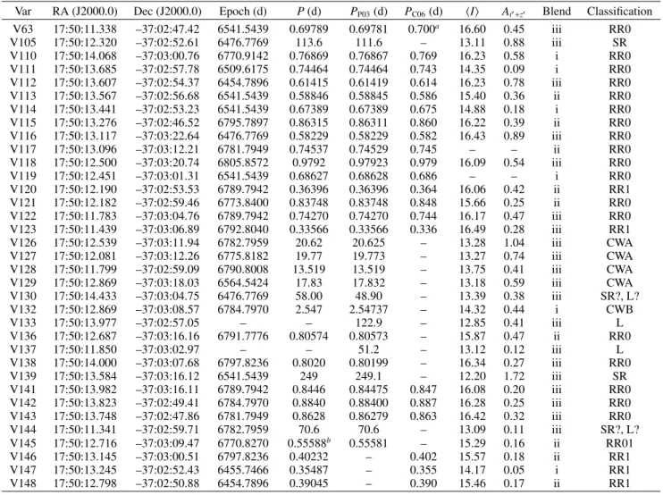
(15) J. Skottfelt et al.: Variable stars in metal-rich globular clusters Table 7. NGC 6441: details of the 49 new variables found in the cluster. Var V151 V152 V153 V154 V155 V156 V157 V158 V159 V160 V161 V162 V163 V164 V165 V166 V167 V168 V169 V170 V171 V172 V173 V174 V175 V176 V177 V178 V179 V180 V181 V182 V183 V184 V185 V186 V187 V188 V189 V190 V191 V192 V193 V194 V195 V196 V197 V198 V199. RA (J2000.0) 17:50:11.983 17:50:12.843 17:50:12.767 17:50:13.338 17:50:13.231 17:50:11.357 17:50:11.670 17:50:13.637 17:50:13.147 17:50:13.536 17:50:12.645 17:50:14.220 17:50:13.742 17:50:11.919 17:50:12.027 17:50:13.434 17:50:14.037 17:50:13.980 17:50:13.918 17:50:13.625 17:50:13.065 17:50:14.561 17:50:14.253 17:50:12.059 17:50:11.371 17:50:12.222 17:50:14.376 17:50:12.930 17:50:12.822 17:50:12.433 17:50:14.294 17:50:13.165 17:50:11.939 17:50:12.906 17:50:11.845 17:50:13.911 17:50:12.583 17:50:12.364 17:50:14.453 17:50:13.032 17:50:13.309 17:50:13.406 17:50:12.269 17:50:13.902 17:50:13.649 17:50:11.542 17:50:11.861 17:50:13.173 17:50:12.346. Dec (J2000.0) –37:03:11.63 –37:03:03.48 –37:03:16.58 –37:03:01.06 –37:03:10.93 –37:03:13.57 –37:03:14.69 –37:02:48.90 –37:03:06.55 –37:03:20.37 –37:03:12.61 –37:02:50.97 –37:03:03.30 –37:03:11.12 –37:03:10.81 –37:02:54.72 –37:03:02.88 –37:03:12.93 –37:03:25.06 –37:03:08.13 –37:02:58.75 –37:03:14.81 –37:03:04.74 –37:02:51.54 –37:03:23.18 –37:03:04.85 –37:03:19.09 –37:02:56.26 –37:03:04.36 –37:03:12.24 –37:03:15.36 –37:03:08.78 –37:02:52.42 –37:03:19.30 –37:03:00.62 –37:03:15.79 –37:02:49.07 –37:03:24.91 –37:03:08.15 –37:03:00.01 –37:03:04.07 –37:03:06.76 –37:03:10.06 –37:03:05.68 –37:02:53.87 –37:02:56.76 –37:02:49.20 –37:02:56.04 –37:02:57.29. Epoch (d) 6564.5424 6564.5424 6541.5439 6455.7466 6564.5424 6789.7942 6775.8182 6784.7970 6782.7959 6795.7897 6564.5424 6770.8270 6546.5297 6564.5424 6564.5424 6546.5297 6789.7942 6789.7942 – – – – – – – – – – – – – – – – – – – – – – – – – – – – – – –. P (d) 0.48716 0.9432 9.89 10.83 11.45 11.76 15.10 17.50 18.5 20.3 24.6 29.3 41.03 41.14 51.6 52 86 128 – – – – – – – – – – – – – – – – – – – – – – – – – – – – – – –. hIi 16.46 – 13.72 13.57 13.03 13.97 13.71 13.89 13.03 13.31 12.95 13.68 12.59 14.37 12.86 12.83 12.78 13.13 12.99 12.89 12.71 13.06 13.10 13.06 13.27 12.65 13.35 12.91 12.72 13.72 13.73 12.62 12.72 12.84 13.07 13.17 13.25 13.70 13.81 13.04 12.46 12.80 13.19 13.19 13.41 13.81 14.07 13.13 13.46. Ai0 +z0 0.80 – 0.15 0.15 0.04 0.03 0.04 0.05 0.06 0.11 0.09 0.06 0.11 0.27 0.21 0.17 0.13 0.11 0.68 0.48 0.29 0.21 0.16 0.14 0.14 0.11 0.09 0.08 0.07 0.07 0.07 0.06 0.06 0.06 0.06 0.06 0.06 0.06 0.06 0.05 0.04 0.04 0.04 0.04 0.04 0.04 0.04 0.03 0.03. Blend iii i iii iii iii iii iii iii ii iii iii iii iii ii iii iii iii iii iii iii iii iii iii iii iii iii iii iii ii iii iii iii iii iii iii iii iii iii iii iii iii iii iii ii iii iii iii iii iii. Classification RR0 RR0? CWA CWA ? SRa SRa SRa SRa SR SR SR SR? ? SR SR SR SR L L L L L L L L L L L L L L L L L L L L L L L L L L L L L L L. Notes. The celestial coordinates correspond to the epoch of the reference image, which is the HJD ∼ 2 456 541.54 d. Epochs are (HJD – 2 450 000). hIi denotes mean I magnitude and Ai0 +z0 are the amplitudes found in our special i0 + z0 filter. The blend column describes whether the star is blended with (i) brighter star(s); (ii) star(s) of similar magnitude; or (iii) fainter/no star(s). (a) These stars have shorter periods than expected for stars of the SR class, but it is not clear how to otherwise classify them according to the GCVS schema given their position on the RGB.. assigned variable numbers V10-V12, respectively, by Clement (priv. comm.). Seven of the X-ray sources lie within our FoV (sources B-E and G-H). Only sources B and H show signs of variability in our difference images and for the remaining sources we cannot find any clear optical counterparts in our reference image at the positions given by Coomber et al. (2011) and Stacey et al. (2012), although we note that our limiting magnitude is ∼19.5 mag (see Fig. 20).. of the stars within our FoV with the variables overplotted. Figure 20 shows the rms magnitude deviation for the 1098 stars with calibrated I magnitudes versus their mean magnitude. The light curves of the variables are plotted in Fig. 21 and their details may be found in Table 11.. A finding chart for the cluster containing the variables detected in this study is shown in Figs. 18 and 19 shows a CMD. V11 (source B) was found by Coomber et al. (2011) to be undergoing rapid X-ray flaring on time scales of less than 100 s.. 3.5.2. Known variables. A103, page 15 of 23.
(16) A&A 573, A103 (2015). I. 15.5. V152 P=0.9432. 0.0. 0.5. 1.0. V156 P=11.76. -5.0 13.68. 0.0. 0.5. 1.0. V157 P=15.10. 0.5. 1.0. V161 P=24.6. 0.0. 0.5. 1.0. 1.0. 13.91. 0.0 12.99. V158 P=17.50. 0.5. 1.0. 13.01. 0.5. 1.0. V163 P=41.03. 13.32 0.0. 0.5. 1.0. V164 P=41.14. 14.2. 12.7. 14.3. 12.8. 12.96. 12.6. 14.4. 12.64. 12.9. 13.7. 14.5. I. 12.56. 13.68. I. 0.5. 1.0. 0.0 12.7. V166 P=52. 0.5. 1.0. 0.5. 1.0. V171. I. 12.6. 6450. 6500. 6550. V176. 0.5. 1.0. 0.0 13.0. V172. 0.5. 1.0. V173. 0.5. 1.0. 6500. 6550. 6800. V177. I. 6500. 6550. 6800. 13.72 13.76 6450. 6500. 6550. 6450. 6550. 6800. V191. 6500. 6550. 6800. 6450. 6500. 6550. 6550. 6800. 6450. 6500. 6550. 6800. V179. 13.35 6450 13.68. 6500. 6550. 6800. 6450 12.8. V183. 6500. 6550. 6800. 6450 13.66. 6500. 6550. 6800. V188. 13.76. 13.23. 13.68. 13.78. 13.25. 13.7. 13.8. 13.27. 13.72. 12.77. 6450. 6500. 6550. 6800. V192. 6500. 6550. 6800. V193. 6550. 6800. V197. 6500. 6550. 6800. 6500. 6550. 6800. 13.21 13.435. V198. 13.12. 13.445. 13.13. 13.455. 13.14 6450. 6550. 6800. 6500. 6550. 6800. 6550. 6800. 6500. 6550. 6800. 6500. 6550. 6800. 6500. 6550. 6800. V185. 6450 13.0. V190. 13.02 13.04 13.06 6450. 6500. 6550. 6800. 6450 13.38. V194. V195. 13.4 13.42. 6450 13.11. 6500. V189. 13.19. 13.21 6500. 13.84 13.17. 13.19. 6450. 6450. 13.82 6450. 13.17. 6500. V180. 6450 13.03. V184. 13.09. 6800. 6800. 13.72. 12.86. 6550. 6550. 12.74. 12.74 6500. 6500. 13.25. 12.64 V187. 1.0. V175. 13.05. 14.08 6500. 6450. 13.07. 14.06. 6450. 6800. 12.82. 14.04. 13.81. 6550. 12.84. 6800. V196. 6500. V174. 12.7. 12.81. 12.47. 6450. 12.72 6450. 0.5. V170. 12.7. 6450 12.68. V182. 12.79. 12.45. V178. 12.66. 1.0. 12.8. 12.6. 13.21. 6500. 6800. 0.5 V165 P=51.6. 13.0. 12.62 6800. V186. 6550. 12.94 6450. 12.58. V181. 6500. 12.9. 13.38 6450. 6450 12.86. 12.95. 0.0. 0.0 12.6. 13.05. 13.1. 13.34. 12.7. 13.83. 0.0. 6450 13.3. 12.66. 13.79. 12.9. 6800. 12.62. 12.43. 0.0 V169. 13.0. 13.14. 13.1. 12.8. 13.12 13.14 13.16 13.18 13.2. 12.6. 13.0. 12.7. 13.68. 1.0. 13.18 0.0. 12.58. 0.5 V168 P=128. 13.1. 12.8. 12.5. 0.0 13.06. V167 P=86. 1.0. 13.36. 13.66. 0.0. 0.5 V160 P=20.3. 13.28. 13.05 0.0. 0.0 13.24. V159 P=18.5. 13.03. 12.52. V162 P=29.3. 13.64. 12.9. I. 0.5. 13.87. 12.8. I. 13.85. 13.05 0.0. 12.92. 12.7. I. 13.6. 13.89. 13.72 0.0. V155 P=11.45. 13.01 13.03. 13.7. 13.98. I. V154 P=10.83. 13.5. 13.75. 13.96. 12.88. V153 P=9.89. 13.65. 5.0. 16.5. 13.94. I. V151 P=0.48716. 6450. 6500. 6550. 6800. 6500. 6550. 6800. 6450. V199. 13.465 6450. 6500. 6550. 6800. 6450. Fig. 11. NGC 6441: light curves for the new variables in our FoV. Red triangles are 2013 data and blue circles are 2014 data. Error bars are plotted but are smaller than the data symbols in many cases. Light curves with confirmed periods are phased. For those variables without periods the x-axis refers to (HJD – 2 450 000), and the dashed line indicates that the period from HJD 2 456 570 to 2 456 760 has been removed from the plot, as no observations were performed during this time range. Note that V152 is plotted in differential flux units, 103 ADU/s, and not calibrated I magnitudes.. Like Engel et al. (2012), we have detected clear variability in the optical counterpart with an amplitude of up to ∼1.1 mag (see Fig. 21). However, as in previous studies, we cannot find a period on which the light curve can be phased. Stacey et al. (2012) suggest that V11 might be a special type of low mass X-ray binary (LMXB) or a very faint X-ray transient (VFXT). One of the advantages of high frame-rate imaging is that it is possible to achieve a high time-resolution by combining the single exposures into short-exposure images. This technique could A103, page 16 of 23. be applied to V11 to determine the time scale of the optical flickering, but it is too faint to be able to do this with our data. 3.5.3. New variables. We found two new variables in the cluster: V13: this star has the same position as the X-ray source H, and we therefore assume that it is the same star. The star has a.
Figure

+7


Documento similar