UNIVERSIDAD DE VALLADOLID
ESCUELA DE INGENIERIAS INDUSTRIALES
Máster en Ingeniería Industrial
ESTUDIO NÚMERICO DE UN FLUJO
IMCOMPRESIBLE A TRAVES DE UNA
PARTICULA CON RUGOSIDAD
Autor:
Ríos Llamas, Judit
Parra Santos, María Teresa
San Diego State university
TFM REALIZADO EN PROGRAMA DE INTERCAMBIO
TÍTULO:
Numerical study of the incompressible flow around a particle with
roughness
ALUMNO:
Judit Ríos LLamas
Abstract
Estudio mediante simulación en el programa CFD de una partícula con forma de
cilindro circular por la que pasa un flujo incomprensible. Inicialmente, se realiza el
estudio de la partícula con superficie perfectamente lisa para números de Reynolds
de 80 y 240. Posteriormente se hace el estudio de esa misma partícula con
diferentes rugosidades, variando en la superficie la frecuencia en unos casos y el
radio en otros, de nuevo para los números de Reynolds de 80 y 240.
Al comparar los resultados obtenidos de la partícula lisa con las partículas con
variación de radio o variación de frecuencia en su superficie, se observa como el
coeficiente de arrastre, coeficiente principal a tener en cuenta, aumenta cada vez
más conforme se le va añadiendo una rugosidad mayor a la partícula. Otros
coeficientes como el de presión, el de elevación y la velocidad, también son
estudiados.
Keywords
NUMERICAL STUDY OF
THE INCOMPRESSIBLE FLOW
AROUND A PARTICLE WITH ROUGHNESS
A Thesis
Presented to the
Faculty of
San Diego State University
In Partial Fulfillment
of the Requirements for the Degree
Master of Science in Aerospace Engineering
by
Abstract
The main objective is the study of a circular cylinder when the cylinder has a wavy wall. For this reason, the influence of a change in frequency and radius for the cylinder wall are investigated.
Contents
Abstract i
List of Figures iv
List of Tables v
1 Introduction 1
2 Governing equations and Computational model 6
3 Results and discussion 9
3.1 Circular cylinder with different Reynolds numbers . . . 9
3.1.1 Drag coefficient . . . 9
3.1.2 Lift coefficient . . . 10
3.1.3 Velocity . . . 11
3.1.4 Pressure . . . 13
3.2 Circular cylinder with a wavy wall when Reynolds number is 240 . . . 15
3.2.1 Radius variation to Reynolds number of 240 . . . 15
3.2.2 Frequency variation to Reynolds number of 240 . . . 20
3.3 Circular cylinder with a wavy wall when Reynolds number is 80 . . . 25
3.3.1 Radius variation to Reynolds number of 80 . . . 25
3.3.2 Frequency variation to Reynolds number of 80 . . . 28
4 Conclusions 31
List of Figures
1 Images of flow patterns that pass around a cylinder [4] a) Re=0.01 b) Re=20 c)Re=75 1
2 Flow patterns that pass around a cylinder [3] a) For Reynolds numbers less than 4 b)
For Reynolds number between 4 and 47 c) For Reynolds number between 47 and 2000. 2
3 Strouhal number as a function of the Reynolds number for a long circular cylinder [6]. 2
4 Drag coefficient as a function of the Reynolds number for a long circular cylinder [1] . 3
5 Graphic representation of base suction coefficient (-CpB) over Reynolds number [7]. . 4
6 Symmetrically placed vortices [7]. . . 4
7 Geometry and boundary conditions used to carry out the study . . . 7
8 Grid used . . . 8
9 Zoom of grid used . . . 8
10 Comparison between graphic representation of the drag coefficient when Reynolds num-ber is 80 and 240 for a circular cylinder with smooth wall . . . 9
11 Graphic representation of the drag coefficient versus Reynolds number. Comparison of dates between literature and simulation. . . 10
12 Comparison between the lift coefficient to circular cylinder with smooth wall when Reynolds number is 80 and Reynolds number is 240. . . 10
13 a) Contour of velocity to Reynolds number of 80. b) Contour of velocity to Reynolds number of 240 . . . 11
14 a) Vorticity contour with maximum velocity 100m/s to Reynolds number 80 for a circular cylinder with a smooth wall. b) Vorticity contour with maximum velocity 100m/s to Reynolds number 240 for a circular cylinder with a smooth wall . . . 11
15 Graphic representation of the normalized velocity . . . 12
16 Graphic representation of Area-Weighted Average Velocity Magnitude over flow time when Reynolds number is 80 for a circular cylinder with a smooth wall. . . 12
17 a) Contour of pressure to Reynolds number of 80 b)Contour of pressure to Reynolds number of 240 . . . 13
18 a) Contour zoom of pressure when Reynolds number is 80 b)Contour zoom of pressure when Reynolds number is 240 . . . 13
19 Plot of the pressure coefficient over position around circular cylinder . . . 14
20 Graphic representation of Mass-Weighted Average Pressure Coefficient over flow time when Reynolds number is 80 and 240 for a circular cylinder with a smooth wall. . . . 14
21 Circular cylinder cases with frequency value 16 and different radius. a) Case R1: radius of 0.0008 b) Case R2: radius of 0.002 c) Case R3: radius of 0.005 d) Case R4: radius of 0.01 . . . 15
22 Graphic representation of the drag coefficient for the different radius cases to Reynolds number of 240 . . . 15
23 Graphic representation of the lift coefficient for the different radius cases when Reynolds number is 240. . . 16
24 Graphic representation of normalized velocity for the different cases of radius to Reynolds number of 240 . . . 17
25 Graphic representation of Area-Weighted Average Velocity Magnitude over flow time when Reynolds number is 240 for a circular cylinder with different radius. . . 17
26 Graphic representation of average pressure coefficient for the different cases of the radius when Reynolds number is 240 . . . 18
28 Circular cylinder cases with radius value of 0.01 and different frequency. a) Case F1: frequency of 6 b) Case F2: frequency of 16 c) Case F3: frequency of 32 d) Case F4:
frequency of 64 . . . 20
29 Graphic representation of the drag coefficient for the frequency cases when Reynolds
number is 240. . . 20
30 Graphic representation of the lift coefficient for different frequencies when Reynolds
number is 240. . . 21
31 Graphic representation of normalized velocity for the different cases of frequency when
Reynolds number is 240. . . 22
32 Graphic representation of Area-Weighted Average Velocity Magnitude over flow time
when Reynolds number is 240 for a circular cylinder with different frequencies. . . 22
33 Graphic representation of average pressure coefficient for the different frequency cases
when Reynolds number is 240 . . . 23
34 Graphic representation of Mass-Weighted Average Pressure Coefficient over flow time
for frequency cases when Reynolds number is 240. . . 24
35 Graphic representation of the drag coefficient for the different radius case when Reynolds
number is 80 . . . 25
36 Graphic representation of the lift coefficient for the radius cases when Reynolds number
is 80 . . . 26
37 Graphic representation of normalized velocity for the different cases of radius when
Reynolds number is 80 . . . 26
38 Graphic representation of average pressure coefficient for the different cases of the radius
when Reynolds number is 80 . . . 27
39 Graphic representation of the drag coefficient for different frequency variations when
Reynolds number is 80 . . . 28
40 Graphic representation of the lift coefficient for different frequency variations when
Reynolds number is 80 . . . 29
41 Graphic representation of normalized velocity for the different cases of frequency when
Reynolds number is 80. . . 29
42 Graphic representation of average pressure coefficient for the different cases of frequency
List of Tables
1 Average drag coefficient values when Reynolds number is 80 and 240 for a circular
cylinder with smooth wall. . . 9
2 Drag coefficient error rate . . . 10
3 Average values of Area-Weighted Average Velocity Magnitude over flow time when
Reynolds number is 80 and 240 for a circular cylinder with a smooth wall. . . 12
4 Average values of Mass-Weighted Average Pressure Coefficient over flow time when
Reynolds number is 80 and 240 for a circular cylinder with a smooth wall. . . 14
5 Average of the drag coefficient value for the different cases of radius when Reynolds
number is 240. . . 16
6 Strouhal number for the different radius cases when Reynolds number is 240 . . . 16
7 Average values of Area-Weighted Average Velocity Magnitude over flow time when
Reynolds number is 240 for a circular cylinder with different radius. . . 18
8 Maximum Pressure Coefficient for radius cases when Reynolds number is 240 . . . 18
9 Average values of Mass-Weighted Average Pressure Coefficient over flow time when
Reynolds number is 240 for radius cases. . . 19
10 Average values of drag coefficient for different frequencies when Reynolds number is 240 21
11 Strouhal number for the cases of frequency when Reynolds number is 240 . . . 21
12 Average values of Area-Weighted Average Velocity Magnitude for the different cases of
frequency when Reynolds number is 240 . . . 23
13 Maximum pressure coefficient along the circular cylinder wall for the cases with different
frequencies to Reynolds number of 240. . . 23
14 Average values of Mass-Weighted Average Pressure Coefficient over flow time for
fre-quency cases when Reynolds number is 240. . . 24
15 Average value of drag coefficient for the different cases of the radius when Reynolds
number is 80. . . 25
16 Maximum Pressure Coefficient for the radius cases when Reynolds number is 80 . . . . 27
17 Average values of drag coefficient for different frequency variations when Reynolds
number is 80 . . . 28
18 Maximum Pressure coefficient for the cases with different frequency when Reynolds
1
Introduction
Considering that the majority of situations in which the interaction of a flow with a nearby object occurs, the object does not have a simple geometry, it has a complex geometry. The main objective is to investigate how the different parameters are affected when we go from a perfectly round and smooth particle to a particle with different roughness. For this reason, the direct numerical simulation is used, simulating the behavior of a fluid around different particles. Therefore, it is a fundamental study of the wake formed when flow passes around particles with different roughness.
The investigation of the behavior of a fluid around a circular cylinder has been carried out by different studies. Previous investigation will be discussed in the next part.
Strouhal [5] developed the first experiment in 1878. This experiment was based on wire experi-encing vortex shedding and sound in the wind. To develop, Strouhal connected a wire between two holders and move it through the air. He realized that neither the wire tension nor its type of material nor its length influenced the vortexes and the sound of the wind produced. It was only affected by the speed with which the wire moved through the air and its diameter. He also concluded that increasing the speed or the diameter of the wire, the vortexes produced become more complex and later will even become turbulent. This wake was named Karman Vortex Street.
The characteristics of a flow past a circular cylinder which is perpendicular to the flow may be classified by the Reynolds number regime. Considering that the Reynolds number is defined as Re =
U∞d/ν, where U is the free stream velocity, d is a reference length (in this case is the diameter of the
circular cylinder) andν is the kinematic viscosity.
A general scheme of how Karman street is developing is shown in figure 2. When a low velocity flow passes around a cylinder or when the diameter of the cylinder is small enough, the stream lines (representing the lines tangent to the velocity vectors at each point of the fluid) only surround the ob-stacle and continue in the flow direction. In the figure 2a, it is observed how the stream lines surround the circular cylinder and close behind it without causing eddies. By increasing the diameter of the cylinder or at higher relative speeds between the fluid and the object, the fluid begins to accumulate in the upstream part of the cylinder such that the pressure between the front and rear of the cylinder increases. Now, the stream lines do not close behind the cylinder and vortexes are formed downstream of the cylinder. The figure 2b shows the typical scheme for this case, where a pair of counter-rotating vortexes that remain behind the circular cylinder are observed. Finally, when the speed or size of the cylinder is even greater, the vortexes are alternately separated behind the cylinder, as it is shown in the figure 2c. These vortexes are the Karman vortexes. In the figure 1, images of the real situations can be seen.
Figure 2: Flow patterns that pass around a cylinder [3] a) For Reynolds numbers less than 4 b) For Reynolds number between 4 and 47 c) For Reynolds number between 47 and 2000.
In addition to the Reynolds number, another important parameter that describes the karman street is Strouhal number. It gives the frequency of shedding of the vortexes and relates the oscillation of a flow with its average velocity [2]. The Strouhal number is defined as St= fd/U, where f is the flow frequency, d is the characteristic length scale (in this case cylinder diameter), and U is the free-stream flow velocity. To different Reynolds number come different frequencies of shedding of vortex pairs. One can see in the figure 3 the Strouhal number plotted against Reynolds number for the flow passing in a circular cylinder.
Other parameter considered is the drag coefficient, cd. It is defined as a dimensionless quantity that is used to quantify the drag or resistance of an object in a fluid environment. A lower drag coefficient indicates the object will have less aerodynamic or hydrodynamic drag. It is defined by
the following formula: cd = 2Fd/ρu2A, where Fd is the drag force which is by definition the force
component in the direction of the flow velocity,ρis the density of the fluid, u is the flow speed of the
object relative to the fluid and A is the reference area. In the next figure, figure 4, one can be seen the plot of drag coefficient over Reynolds number to circular cylinder:
Figure 4: Drag coefficient as a function of the Reynolds number for a long circular cylinder [1]
The flow behavior also affects the elevation coefficient and the pressure coefficient. The lift coef-ficient (cl) is a dimensionless coefcoef-ficient that relates the lift generated by a lifting body to the fluid density around the body, the fluid velocity and an associated reference area. The lift coefficient is
defined as cl = 2L/ρu2A where, L is lift, ρ is density, u is velocity and A is body area. And the
pressure coefficient is a dimensionless number which describes the relative pressures throughout a flow
field in fluid dynamics. It is defined howcp=p−p∞/12ρ∞U
2
∞=p−p∞/po−p∞ where p is is the
static pressure at the point at which pressure coefficient is being evaluated,p∞is the static pressure
in the free-stream,pois the stagnation pressure in the free-stream,ρ∞is the free-stream fluid density
andU∞ is the free-stream velocity of the fluid.
Several attempts have been made to identify parameters which can uniquely define the behavior of the wake. This is complicated because there are three layers of shear involved that interact with each other: a boundary layer, a separating free layer of shear and a wake [8]. These issues were researched by Williamson [7] and his study described below. Also, Mathis et al. [3] studied these issues, and his work is mentioned.
Williamson classified the flow regimes and the transition regimes according to the base suction
coefficient (−CpB), this coefficient represents the dimensionless pressure at the point 180 degrees
Figure 5: Graphic representation of base suction coefficient (-CpB) over Reynolds number [7].
• Regime up to A: Laminar Steady Regime (Re < 49) In this regimen the wake has a steady
recirculation region of two symmetrically placed vortices on each side of the wake. It can be seen in the figure 6.
Figure 6: Symmetrically placed vortices [7].
• Regime A-B: Laminar Vortex Shedding (49<Re<140-194) The regimen shows a sharp
devi-ation, it is the beginning of the vortices shedding.
• Regime B-C: Wake-transition Regime (190<Re<260) In this region there are two discontinuous
• Regime C-D: Increasing Disorder in the Fine-Scale 3D (260<Re<1000) At the point Re=260 its behave is as laminar shedding mode. Moreover, when Reynolds number increased towards point D in the plot appear an increasing disorder in the fine-scale 3D effects.
• Regime D-E: Shear-Layer Transition Regime (1k<Re<200k) In this region, stability increases
because of the separation of the cutting layers from the sides of the body.
• Regime E-G: Asymmetric Reattachment (200k < Re< 500k) The base suction and the drag
decrease drastically owing to separation-reattachment bubble causing the revitalized boundary layer to separate much further downstream then for the laminar case.
• Regime G-H: Symmetric Reattachment Regime(500k<Re<1M) This region has a supercritical
regimen. For this reason the flow is symmetric with tow separation-reattachment bubbles, one on each side of the body.
• Regime H-J: Boundary-Layer Transition Regime (Re>1M) This regimen is associated with a
sequence of fundamental shear flow instabilities.
On the other hand, Mathis et al. (1984) performed laboratory experiments in an open circuit
wind tunnel with a Doppler laser and determined that vortex shedding occurs for Reynolds numbers
Re>47. In the figure 2 the Mathis et al. values are shown.
Considering both studies, it can be concluded that the shedding starts at Reynolds number of 47-49.
We investigate the influence of particles with different roughness on the flow and wake and how the different parameters are affected by these particles. It is carried out using two different Reynolds num-ber. We can conclude that the behavior of the calculated parameters is the same for both Reynolds number studied. The more roughness the particle has, the more the parameters obtained from the smooth wall results move away
2
Governing equations and Computational model
Governing equations
The CFD software has been used to calculate the flow over a circular cylinder with different roughness. First, we show the governing Reynolds Average Navier-Stokes Equations which Fluent uses as flow model are describing. Secondly, some aspects of the numerical methodology. Finally, the computa-tional model will be described.
Navier-Stokes equations are the governing equations of Computational Fluid Dynamics. It is based on the conservation law of physical properties of fluid. The principle of conservational law is the change of properties, such as mass, energy, and momentum, in an object is decided by the input and output.
Applying the mass, momentum and energy conservation, we can derive the continuity equation, momentum equation and energy equation as follows.
The continuity equation is defined in the expression 1:
Dρ Dt +ρ
∂Ui
∂xi
= 0 (1)
The momentum equation is show in the expression 2, where the first term isLocal change with time,
the second term ismomentum convection, the third term isSurface force, the fourth term is
Molecular-dependent momentum exchange (diffusion)and the last one term isMass force.
ρ∂Uj ∂t +ρUi
∂Uj
∂xi
=−∂P
∂xj
−∂τij
∂xi
+ρgj (2)
The energy equation is defined in the nest expression, expression 3. Its terms are the following
ones in the same order: Local energy change with time, Convective term, Pressure work, Heat flux
(diffusion)and Irreversible transfer of mechanical energy into heat
ρcµ
∂T
∂t +ρcµUi ∂T ∂xi
=−P∂Ui
∂xi
+λ∂
2T
∂x2
i
−τij
dUj
∂xi
(3)
Computational model
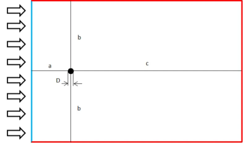
The physical domain developed and used is shown in the figure 7. This physical domain is a rectangle with dimensions 50x70m. The circular cylinder diameter is defined as D and is located in middle of the domain. The distance between the inlet and the circular cylinder is defined as ‘a’ and its length is 7 meters, ‘c’ whose value is 57 meters is the length between the circular cylinder and the outlet on the right, and the length between circular cylinder and the up and down outlets is defined as ‘b’ and its length is 22 meters.
Furthermore, in the figure 7, we can see the boundary conditions which are:
• Inlet (blue line): velocity-inlet. At the inlet the inflow is homogeneous and uniform.
• Outlet (red line): outflow
• Circular cylinder: wall
Figure 7: Geometry and boundary conditions used to carry out the study
The value of circular cylinder diameter will be 1m, the value of the viscosity will be 1 kg/(m·s) and
the value of the density will be 1 kg/m3 in all cases. Therefore, when the velocity is 80, the Reynolds
number is 80 and when the velocity is 240, the Reynolds number is 240.
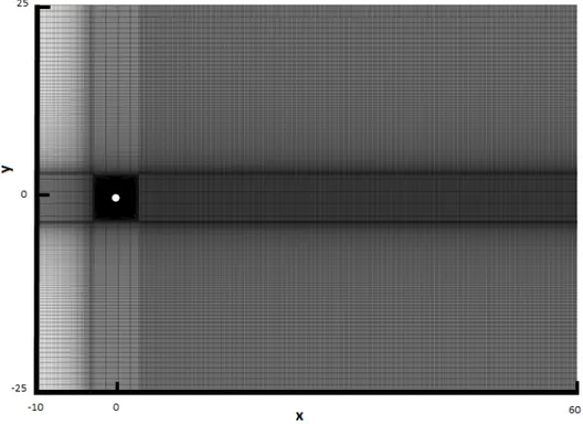
Figure 8: Grid used
3
Results and discussion
3.1
Circular cylinder with different Reynolds numbers
The study of the circular cylinder with a smooth wall is carried out with the two Reynolds numbers, 80 and 240. The results are shown below.
3.1.1 Drag coefficient
Figure 10 and table 1 show the graphic representation of the drag coefficient and its average values respectively. For Reynolds numbers of 80 the oscillation amplitude is lower than for Reynolds number of 240.
1.15 1.2 1.25 1.3 1.35
Cd
flow time (s)
Re80 Re240
Figure 10: Comparison between graphic representation of the drag coefficient when Reynolds number is 80 and 240 for a circular cylinder with smooth wall
Case Reynolds number Average drag coefficient
1 80 1.3768
2 240 1.2019
Table 1: Average drag coefficient values when Reynolds number is 80 and 240 for a circular cylinder with smooth wall.
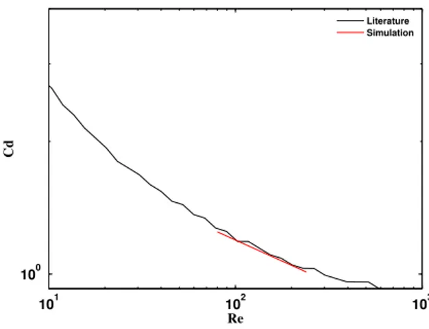
Validate the results against literature.
101 102 103 100
Cd
Re
Literature Simulation
Figure 11: Graphic representation of the drag coefficient versus Reynolds number. Comparison of dates between literature and simulation.
Case Re Average Cd simulation Cd literature error rate
1 80 1.3768 1.4127 2.54
2 240 1.2019 1.2201 1.49
Table 2: Drag coefficient error rate
3.1.2 Lift coefficient
The lift coefficient graphic representation for the two Reynolds numbers is shown in figure 12. The amplitude and the frequency of the oscillation is higher for Reynolds number of 240 than for Reynolds number of 80.
62.2 62.3 62.4 62.5 62.6 62.7 −0.4
−0.3 −0.2 −0.1 0 0.1 0.2 0.3 0.4
Cd
flow time (s)
Re80 Re240
3.1.3 Velocity
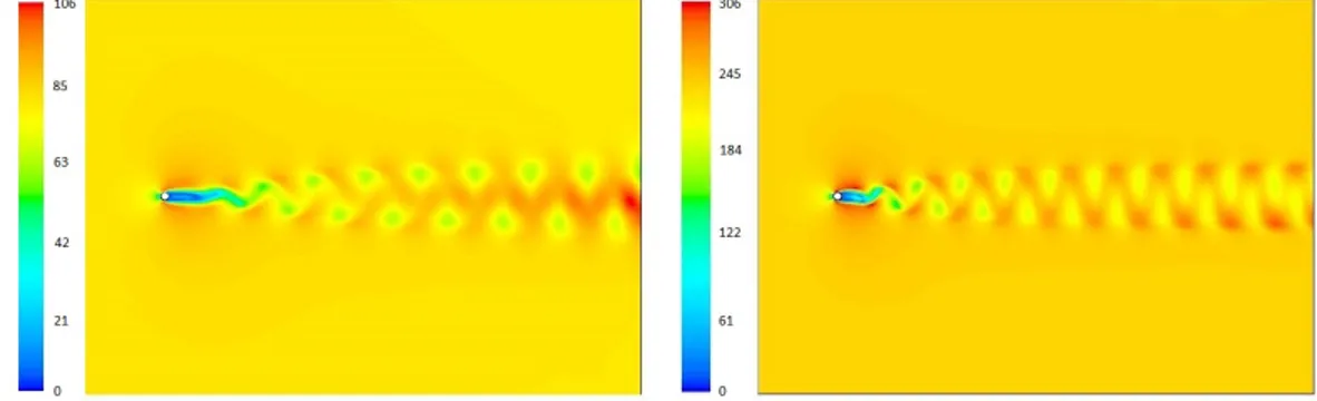
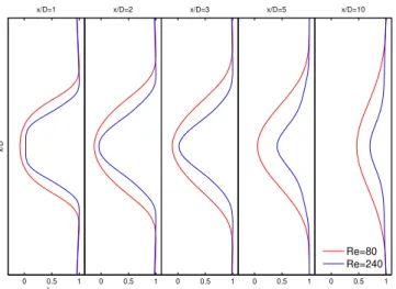
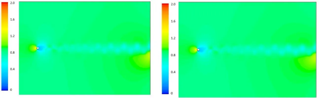
The velocity contours for both cases, Reynolds number of 80 and Reynolds number of 240, are repre-sented in the figure 13. We can appreciate that for higher Reynolds numbers the Karman street has higher frequencies of vortex pairs.
Figure 13: a) Contour of velocity to Reynolds number of 80. b) Contour of velocity to Reynolds number of 240
The vorticity contours are shown in the figure 14, where we can see that for the higher Reynolds value the vorticity contour has a more pronounced Karman street
Figure 14: a) Vorticity contour with maximum velocity 100m/s to Reynolds number 80 for a circular cylinder with a smooth wall. b) Vorticity contour with maximum velocity 100m/s to Reynolds number 240 for a circular cylinder with a smooth wall
0 0.5 1
u*
x/D
x/D=1
0 0.5 1
x/D=2
0 0.5 1
x/D=3
0 0.5 1
x/D=5
0 0.5 1
x/D=10
Re=80 Re=240
Figure 15: Graphic representation of the normalized velocity
The graphic representations of Area-Weighted Average Velocity Magnitude over flow time for both cases are shown in the figure 16. The average values of this representation are shown in the table 3.
79.24 79.241 79.242 79.243 79.244 79.245 79.246 79.247 79.248
Area−Weighted Average Velocity Magnitude
flow time (s)
Case 80 238.9 238.95 239 239.05 239.1 239.15
Area−Weighted Average Velocity Magnitude
flow time (s)
Re240
Figure 16: Graphic representation of Area-Weighted Average Velocity Magnitude over flow time when Reynolds number is 80 for a circular cylinder with a smooth wall.
Case Re Average of Area-Weighted Average Velocity Magnitude
1 80 79.2436
2 240 239.0498
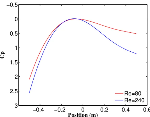
3.1.4 Pressure
The figure 17 shows the pressure coefficient contours for the both Reynolds numbers studied, 80 and 240.
Figure 17: a) Contour of pressure to Reynolds number of 80 b)Contour of pressure to Reynolds number of 240
Figure 18 is obtained by zooming in the previous contours of the pressure coefficient. In this figure, we can appreciate how the pressure behaves on the circular cylinder wall.
Figure 18: a) Contour zoom of pressure when Reynolds number is 80 b)Contour zoom of pressure when Reynolds number is 240
−0.4 −0.2 0 0.2 0.4 0.6 −0.5
0
0.5
1
1.5
2
2.5
3
Cp
Position (m)
Re=80 Re=240
Figure 19: Plot of the pressure coefficient over position around circular cylinder
In the figure 20 we can see the graphic representation of Mass-Weighted Average Pressure Coeffi-cient over flow time. The average values of this representation are shown in the table 4.
0.6 0.7 0.8 0.9 1 1.1 1.2 1.3 1.4 1.5
Mass−Weighted Average Pressure Coefficient
flow time (s)
Re80
Re240
Figure 20: Graphic representation of Mass-Weighted Average Pressure Coefficient over flow time when Reynolds number is 80 and 240 for a circular cylinder with a smooth wall.
Case Re Average of Mass-Weighted Average Pressure Coefficient
1 80 0.88848
2 240 1.1758
3.2
Circular cylinder with a wavy wall when Reynolds number is 240
3.2.1 Radius variation to Reynolds number of 240
The circular cylinder study has been carried out for four different radius with the same frequency value, 16. The different cases are shown in the figure 21:
Figure 21: Circular cylinder cases with frequency value 16 and different radius. a) Case R1: radius of 0.0008 b) Case R2: radius of 0.002 c) Case R3: radius of 0.005 d) Case R4: radius of 0.01
The obtained results are shown bellow.
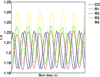
Drag coefficient
In figure 22 and table 5 show the graphic representation and the average drag coefficient values respectively. It can been appreciated that the variation of the drag coefficient is very little. When radius value increases, the value of the drag coefficient increases too, moving away from the drag coefficient value for the circular cylinder. However, it is appreciated in the case R1 that when the radius increases a very little, the value of the drag coefficient is similar to circular cylinder case.
1.18 1.19 1.2 1.21 1.22 1.23 1.24 1.25
Cd
flow time (s)
CC R1 R2 R3 R4
Case Radius Frequency Average drag coefficient
Circular cylinder - - 1.2019
Case R1 0.0008 16 1.2018
Case R2 0.003 16 1.2024
Case R3 0.005 16 1.2081
Case R4 0.01 16 1.2210
Table 5: Average of the drag coefficient value for the different cases of radius when Reynolds number is 240.
Lift coefficient
Figure 23 shows the graphic representation of the lift coefficient. One can see that the oscillation amplitude is similar but oscillation frequency varies for the different cases.
−0.4 −0.3 −0.2 −0.1 0 0.1 0.2 0.3 0.4
Cl
flow time (s)
CC R1 R2 R3 R4
Figure 23: Graphic representation of the lift coefficient for the different radius cases when Reynolds number is 240.
The value of period, oscillation frequency and Strouhal number to the different cases are shown in table 6, where one can see that the Strouhal number varies very little.
Cases Period Oscillation frequency Strohual number
Circular cylinder 0.02470 40.493 0.1687
Case R1 0.02467 40.541 0.1689
Case R2 0.02465 40.565 0.1690
Case R3 0.02468 40.512 0.1688
Case R4 0.02479 40.340 0.1681
velocity
The figure 24 shows the normalized velocity (u*) for the different cases in the position x/D= 1, 2, 3, 5 and 10. The value of normalized velocity is a little less when the radius increases although its variation is very small.
0 0.5 1 −2 −1.5 −1 −0.5 0 0.5 1 1.5 2 u* x/D
x/D=1 x/D=2 x/D=3 x/D=5 x/D=10
CC R1 R2 R3 R4
Figure 24: Graphic representation of normalized velocity for the different cases of radius to Reynolds number of 240
The average velocity over flow time for the four radius cases is represented in the figure 25 and its average values are shown in the table 7. These values practically do not vary.
238.9 238.95 239 239.05 239.1 239.15
Area−Weighted Average Velocity Magnitude
flow time (s)
CC R1 R2 R3 R4
Cases Average Area-Weighted Average Velocity Magnitude
Circular cylinder 239.050
Case R1 239.018
Case R2 239.067
Case R3 239.018
Case R4 239.051
Table 7: Average values of Area-Weighted Average Velocity Magnitude over flow time when Reynolds number is 240 for a circular cylinder with different radius.
Pressure
In figure 26, we can see the average pressure coefficient along the wall of cylinder. It is appreciated that when the radius increases the amplitude and frequency of oscillation increase too.
−0.4 −0.2 0 0.2 0.4 0.6
−1
−0.5
0
0.5
1
1.5
2
2.5
3
Cp
Position (m)
CC R1 R2 R3 R4
Figure 26: Graphic representation of average pressure coefficient for the different cases of the radius when Reynolds number is 240
The value of the maximum pressure coefficients for the different cases are shown in the table 8. This value is lower when radius increases.
Cases Maximum Pressure Coefficient
Circular cylinder 2.55
Case R1 2.38
Case R2 2.34
Case R3 2.28
Case R4 2.22
The graphic representation of Mass-Weighted Average Pressure Coefficient over flow time is shown in the figure 27. The average values of this representation are shown in the table 9 and its value is smaller when the radius is increased.
0.7 0.8 0.9 1 1.1 1.2 1.3
Mass−Weighted Average Velocity Magnitude
flow time (s)
CC R1 R2 R3 R4
Figure 27: Graphic representation of Mass-Weighted Average Pressure Coefficient over flow time when Reynolds number is 240 for radius cases.
Case Average of Mass-Weighted Average Pressure Coefficient
Circular cylinder 1.1758
Case R1 1.0480
Case R2 1.0597
Case R3 0.0569
Case R4 0.0508
3.2.2 Frequency variation to Reynolds number of 240
The circular cylinder study has been carried out for four different frequencies with the same radius, 0.01. The different cases are shown in the figure 28:
Figure 28: Circular cylinder cases with radius value of 0.01 and different frequency. a) Case F1: frequency of 6 b) Case F2: frequency of 16 c) Case F3: frequency of 32 d) Case F4: frequency of 64
The obtained results are shown bellow.
Drag coefficient
The drag coefficient values to the different cases are shown in figure 29 and table 10. It can been appreciated that when the frequency increases, the value of the drag coefficient increases too.
65.2 65.22 65.24 65.26 65.28 65.3 1.15
1.2 1.25 1.3 1.35 1.4
Cd
flow time (s)
CC F1 F2 F3 F4
Case Radius Frequency Average drag coefficient
Circular cylinder - - 1.2019
Case F1 0.01 6 1.2152
Case F2 0.01 16 1.2210
Case F3 0.01 32 1.2248
Case F4 0.01 64 1.3422
Table 10: Average values of drag coefficient for different frequencies when Reynolds number is 240
Lift coefficient
Figure 30 shows the graphic representation of the lift coefficient. The oscillation amplitude for the lift coefficient is similar in all the cases but its oscillation frequency varies.
−0.4 −0.3 −0.2 −0.1 0 0.1 0.2 0.3 0.4
Cl
flow time (s)
CC F1
F2 F3 F4
Figure 30: Graphic representation of the lift coefficient for different frequencies when Reynolds number is 240.
The value of period, oscillation frequency and Strouhal number to frequency cases are shown in the table 11. It can be seen the Strouhal number varies very little when the circular cylinder increases its roughness.
Cases Period Oscillation frequency Strohual number
Circular cylinder 0.02470 40.493 0.1687
Case F1 0.02469 40.502 0.1688
Case F2 0.02479 40.340 0.1681
Case F3 0.02484 40.254 0.1677
Case F4 0.02632 38.000 0.1583
Velocity
The figure 31 shows the normalized velocity (u*) for the cases in the position x/D= 1, 2, 3, 5 and 10. One can see that the value of the normalized velocity is smaller when the circular cylinder has frequencies in its wall, although the difference is very small.
u*
x/D
x/D=1 x/D=2 x/D=3 x/D=5 x/D=10
CC F1 F2 F3 F4
Figure 31: Graphic representation of normalized velocity for the different cases of frequency when Reynolds number is 240.
The graphic representation of average velocity over flow time and its average velocity values can be seen in figure 32 and in table 12. These values vary very little.
238.9 238.95 239 239.05 239.1 239.15
Area−Weighted Average Velocity Magnitude
flow time (s)
CC R1 R2 R3 R4
Cases Average Area-Weighted Average Velocity Magnitude
Circular cylinder 239.0498
Case F1 239.0486
Case F2 239.0506
Case F3 238.9826
Case F4 239.1492
Table 12: Average values of Area-Weighted Average Velocity Magnitude for the different cases of frequency when Reynolds number is 240
Pressure
In figure 33, it is appreciate the average pressure coefficient along the wall of cylinder. The more frequency the circular cylinder wall has, the more amplitude and frequency of oscillation has the graphic representation.
−0.4 −0.2 0 0.2 0.4 0.6
−4
−3
−2
−1
0
1
2
3
Cp
Position (m)
CC R1 R2 R3 R4
Figure 33: Graphic representation of average pressure coefficient for the different frequency cases when Reynolds number is 240
The value of the maximum pressure coefficient decreases when the circular cylinder wall has fre-quency. These values are shown in the table 13
Cases Pressure coefficient
Circular cylinder 2.55
Case F1 2.26
Case F2 2.22
Case F3 1.44
Case F4 0.07
The graphic representation of Mass-Weighted Average Pressure Coefficient over flow time is shown in the figure 34. The average values of this representation are shown in the table 14 and its value is smaller when the frequency increases.
62.5 62.55 62.6 62.65 62.7
−1 −0.5 0 0.5 1 1.5
Mass−Weighted Average Pressure Coefficient
flow time (s)
CC F1 F2 F3 F4
Figure 34: Graphic representation of Mass-Weighted Average Pressure Coefficient over flow time for frequency cases when Reynolds number is 240.
Case Average of Mass-Weighted Average Pressure Coefficient
Circular cylinder 1.1758
Case F1 1.0803
Case F2 1.0508
Case F3 0.7835
Case F4 -0.9841
3.3
Circular cylinder with a wavy wall when Reynolds number is 80
The same calculations are made next but with Reynolds number of 80 with a different step time. The results are shown below and its behavior is the same as the case with Reynolds number of 240.
3.3.1 Radius variation to Reynolds number of 80
Drag coefficient
The drag coefficients values and its graphic representation are shown in figure 35 and the table 15.
230 230.1 230.2 230.3 230.4 230.5 230.6 230.7 230.8 230.9 231
1.24 1.245 1.25 1.255 1.26 1.265
Cd
flow time (s)
CC F1 F2 F3 F4
Figure 35: Graphic representation of the drag coefficient for the different radius case when Reynolds number is 80
Case Radius Frequency Average drag coefficient
Circular cylinder - - 1.2464
Case R1 0.0008 16 1.2468
Case R2 0.003 16 1.2467
Case R3 0.005 16 1.2492
Case R4 0.01 16 1.2561
Lift coefficient
The figure 36 shows the graphic representation of the lift coefficient for the cases of radius when Reynolds number is 80:
248.3 248.4 248.5 248.6 248.7 248.8 248.9 249 −0.02 −0.015 −0.01 −0.005 0 0.005 0.01 0.015 0.02 0.025 Cl
flow time (s)
CC F1 F2 F3 F4
Figure 36: Graphic representation of the lift coefficient for the radius cases when Reynolds number is 80
Velocity
The figure 37 shows the normalized velocity (u*) for the different cases of radius to Reynolds number of 80 in the position x/D= 1, 2, 3, 5 and 10.
0 0.5 1 −2 −1.5 −1 −0.5 0 0.5 1 1.5 2 u* x/D
x/D=1 x/D=2 x/D=3 x/D=5 x/D=10
CC F1 F2 F3 F4
Pressure
In figure 38, one can see the average pressure coefficient along the wall of cylinder for the four radius cases when Reynolds number is 80. And the values of the maximum pressure coefficients for these cases are shown in the table 16.
−0.4 −0.2 0 0.2 0.4 0.6
−0.5
0
0.5
1
1.5
2
2.5
Cp
Position (m)
CC F1 F2 F3 F4
Figure 38: Graphic representation of average pressure coefficient for the different cases of the radius when Reynolds number is 80
Cases Maximum Pressure Coefficient
Circular cylinder 2.0944
Case R1 2.059
Case R2 2.060
Case R3 2.049
Case R4 2.092
3.3.2 Frequency variation to Reynolds number of 80
Drag coefficient
The drag coefficient graphic representation and its average values to the frequency cases when Reynolds number is 80 are shown in figure 39 and the table 17.
249 249.1 249.2 249.3 249.4 249.5 249.6 249.7 249.8 249.9 250
1.22 1.24 1.26 1.28 1.3 1.32 1.34 1.36 1.38
Cd
flow time (s)
CC F1 F2 F3 F4
Figure 39: Graphic representation of the drag coefficient for different frequency variations when Reynolds number is 80
Case Radius Frequency Average Drag coefficient
Circular cylinder - - 1.2465
Case F1 0.01 6 1.2528
Case F2 0.01 16 1.2561
Case F3 0.01 32 1.2603
Case F4 0.01 64 1.3657
Lift coefficient
The figure 40 shows the graphic representation of the lift coefficient when Reynolds number is 80 in the cases of frequency variations.
231.5 231.55 231.6 231.65 231.7 231.75 231.8 231.85 231.9 231.95 232 −0.03 −0.02 −0.01 0 0.01 0.02 0.03 Cl
flow time (s)
CC F1 F2 F3 F4
Figure 40: Graphic representation of the lift coefficient for different frequency variations when Reynolds number is 80
Velocity
The figure 41 shows the normalized velocity (u*) for the cases in the position x/D= 1, 2, 3, 5 and 10 for the frequency cases when Reynolds number is 80.
0 0.5 1 −2 −1.5 −1 −0.5 0 0.5 1 1.5 2 u* x/D
x/D=1 x/D=2 x/D=3 x/D=5 x/D=10
CC F1 F2 F3 F4
Pressure
In the figure 42 it is appreciate the graphic representation of the average pressure coefficient along the wall of cylinder when Reynolds number is 80 for the frequency cases.
−0.4 −0.2 0 0.2 0.4 0.6
−3
−2
−1
0
1
2
3
Cp
Position (m)
CC F1 F2 F3
F4
Figure 42: Graphic representation of average pressure coefficient for the different cases of frequency when Reynolds number is 80
The value of the maximum pressure coefficient for these cases can see in table 18.
Cases Pressure coefficient
Circular cylinder 2.0944
Case F1 2.0814
Case F2 2.0926
Case F3 1.6261
Case F4 0.2947
4
Conclusions
After having carried out the study of the different particles for Reynolds numbers 80 and 240, it can been concluded that as the roughness of the particle increases, the different parameters move further and further away from the values for a particle with a smooth surface. This behavior happens for both Reynolds number, 80 and 240.
In the case of the drag coefficient, as the more you increase the roughness (radius or frequency) the more the drag coefficient value increases.
While, the amplitude of oscillation in the graphic representation of the lift coefficient is similar for the cases compared, the oscillation frequency varies. Therefore, Strohual number varies.
The normalized velocity varies very little and does so by decreasing its value as the roughness increases. Also, the average velocity varies very little from one case to another for all the cases with the same Reynolds number.
The last parameter treated is the pressure coefficient, the maximum value of this coefficient de-creases when the roughness inde-creases. Furthermore, when the roughness inde-creases, one can see in the graphical representation of the pressure coefficient how the oscillation of its representation increases too. The average pressure coefficient over time decreases when the circular cylinder has roughness.
References
[1] Robert W Fox and Alan T McDonald. Introduction to fluid mechanics, john wiley&sons. Inc.,
New York, 1994.
[2] PK Kundu and IM Cohen. Fluid mechanics, 3rd edn. San Diego, CA, USA: Elsevier Academic
Press, 1:271–377, 2004.
[3] Christian Mathis, Michel Provansal, and Louis Boyer. The b´enard-von k´arm´an instability: an
experimental study near the threshold. Journal de Physique Lettres, 45(10):483–491, 1984.
[4] Gemma Sibera Quilez. Estudio de la calle de von k´arm´an en un cilindro mediante piv. 2013.
[5] V Strouhal. On one particular way of tone generation.Annalen der Physik und Chemie (Leipzig),
ser. 3, 5:216–251, 1878.
[6] Frank M White and Isla Corfield. Viscous fluid flow. 3, 2006.
[7] Charles HK Williamson. Vortex dynamics in the cylinder wake.Annual review of fluid mechanics,
28(1):477–539, 1996.
[8] MM Zdravkovich. Different modes of vortex shedding: an overview. Journal of fluids and
![Figure 3: Strouhal number as a function of the Reynolds number for a long circular cylinder [6].](https://thumb-us.123doks.com/thumbv2/123dok_es/5378189.720315/11.918.213.712.656.955/figure-strouhal-number-function-reynolds-number-circular-cylinder.webp)
![Figure 5: Graphic representation of base suction coefficient (-CpB) over Reynolds number [7].](https://thumb-us.123doks.com/thumbv2/123dok_es/5378189.720315/13.918.140.823.129.612/figure-graphic-representation-base-suction-coefficient-reynolds-number.webp)