Abstract Innovative Families Of Double-Layer Tensegrity Grids: Quastruts and Sixstruts

1

Innovative Families Of Double-Layer Tensegrity Grids: Quastruts and Sixstruts

1

Valentin Gomez-Jauregui 1, Cesar Otero 2, Ruben Arias 3, Cristina Manchado 4 2

3 4

Abstract

5

Double-layer tensegrity grids (DLTG) are spatial reticulated systems based on tensegrity principles, 6

which have been studied in detail over recent years. The most important investigations have been 7

carried out focusing on a short list of tensegrity grids. This paper explains with real examples how 8

to use Rot-Umbela Manipulations, a unique technique developed for generating innovative 9

typologies of tensegrity structures. It is applied to two already existing tensegrity grids in order to 10

obtain two new DLTGs. Their analysis permits us to identify, inside these novel grids, the modules 11

that compose them which were unknown until now. A brief description of these components is 12

provided, as well as some information about their static analysis, e.g. states of self-stress and 13

internal mechanisms. These novel modules belong to a family, all of them with similar 14

characteristics in terms of geometry and topology, and can be used to generate a wide catalogue 15

of DLTGs. Some examples of new grids are presented, describing the methodology on how to 16

obtain many more models for other designers interested in creating and studying innovative 17

DLTGs. 18

1

Corresponding author: B.Eng, MSc Arch. Assistant lecturer, University of Cantabria, Spain.Tel. +34 620 956 969, E-mail address: [email protected]. Dpt. Geographic Engineering and Graphical

Expression Techniques. Avda./ Castros s/n. 39005 Universidad de Cantabria, Spain

2

Dpt. Geographic Engineering and Graphical Expression Techniques. Avda./ Castros s/n. 39005 Universidad de Cantabria, Spain

3

Dpt. Geographic Engineering and Graphical Expression Techniques. Avda./ Castros s/n. 39005 Universidad de Cantabria, Spain

4 _{Dpt. Geographic Engineering and Graphical Expression Techniques. Avda./ Castros s/n. 39005 Universidad}

2

Subject Heading

1

Structural engineering, Architectural engineering, Structural design, Grid systems, Tension 2

structures, Space structures. 3

Keywords

4

tensegrity, structures, double-layer, grids, Rot-Umbela, self-stress, tension, mechanism, Quastrut, 5 Sixstrut 6

Abbreviations

a Amplitude or length of opening of the Rot-Umbela Manipulation 9

b number of nodes 10

C Damping matrix 11

D Force Density matrix 12

dim number of dimensions 13

e number of members 14

f vector of external forces 15

j number of restrictions 16

k Class of tensegrity (maximum number of struts concurring to the same joint) 17

L Length of the cables of top or bottom layer 18

M Mass matrix 19

m Number of internal mechanisms (not including rigid body mechanisms) 20

n Number of struts concurring at each vertex 21

q Force density vector 22

r Rotation of the Rot-Umbela Manipulation 23

3 R Residual Force vector

1

s Number of states of self-stress 2 u Umbela valence 3 v Vertex valence 4 5

4 1

2

Introduction

3

Double-layer tensegrity grids (DLTGs) are tensegrity spatial reticulated systems containing two 4

parallel networks of members in tension forming the top and bottom chords, whose nodes are 5

linked by vertical and/or inclined web members under compression and tension. Even if this 6

concept is clear, definition of Tensegrity has always been very ambiguous and important 7

differences arise depending on different authors. In this paper, tensegrities will be considered as 8

self-stressed and auto-stable structures composed by isolated components in compression inside 9

a net of continuous tension, in such a way that the compressed members (usually bars or struts) 10

do not touch each other and the pre-stressed tensioned members (usually wires or even tensile 11

membranes) delineate the system spatially (Gomez-Jauregui 2010). Compressed elements can be 12

contiguous as long as they are only and always under compression and pin-jointed; in that case, it 13

could be considered that there are not several simple elements under compression, but just one 14

complex component constituted by an assembly of elementary elements in compression (Motro 15

2003). When this happens, k>1, k being the class of the tensegrity, which is the maximum number 16

of struts concurring at one node of the structure (Skelton et al. 1998). 17

Tensegrity structures and, more specifically, DLTGs have been the center of attention of several 18

kinds of engineers (civil, mechanical, electronic, etc.) and architects due to their lightweight, 19

efficiency, deployability and flexibility, among other benefits. Although there are also some 20

disadvantages (cost, complex assembly, high deflections, vibrations, etc.), they have been taken 21

into account frequently for many recent studies and projects (Dalilsafei and Tibert 2012; Knight et 22

al. 2000; Rhode-Barbarigos et al. 2010; Stucchi et al. 2006). Main researches have dealt with their 23

5

application to roofs (Panigrahi et al. 2009), but some others have tried to incorporate them to 1

architecture as double glazing walls (Mitsos et al. 2011). 2

A perspective of the historical proposals for DLTGs over their relatively short history (60 years) has 3

been presented recently (Gomez-Jauregui et al. 2011). However, some important projects in the 4

80s should be remarked upon, like the grid composed by Half-Cuboctahedrons, by Motro (1987), 5

who studied a grid composed by quadrangular tensegrity pyramids (mainly the same modules 6

showed by Emmerich (1964) in his first patent), by means of joining the ends of their struts. The 7

possibilities offered by the juxtaposition of simple tensegrity modules (with 3, 4, 5 and 6 struts), 8

were analyzed by Hanaor (1991), experiencing with the composition of tensegrity prisms (for 9

planar systems) and truncated pyramids (for domical configurations), avoiding contacts between 10

struts. A large catalogue was created by Emmerich (1988) by combinational assembly of tensegrity 11

prisms and pyramids, which is also an inspiration for the development of the last section of this 12

paper. He mainly used prismatic, anti-prismatic, anti-pyramidal, interlaced and inter-penetrated 13

tensegrity modules, creating several and variable tessellations. In the next decade, Kono and 14

Kunieda (1996) designed an original DLTG composed by tripod-like modules and patented it as long 15

as some of its variations. Different geometries were tested, depending on the attachments of the 16

wires of the bigger base (direct to the edges of the struts, to the gravity center of the base or to 17

some intermediate points of the bisectrices of the base). A big-scale model composed by 33 18

triangular modules, with an 80m2 covered area, was constructed at the end of the experiment, 19

including a newly proposed member joint system for their assembly. However, maybe one of the 20

most important breakthroughs was achieved by Vinicius Raducanu (2001), who was integrated into 21

the Tensarch project at the LMGC of University of Montpellier. In his PhD thesis, he proposed a new 22

methodology for creating tensegrity grids by means of the use of interdependent expanders instead 23

of independent auto-stable modules, applying topological and geometrical relationships between 24

6

them. This innovative technique lead to an important step forward, obtaining new forms never 1

found before, materialized on 15 new grids and a new line of research for future studies. 2

Recently, the authors of the present work have also proposed a new approach for generating new 3

DLTGs (Gomez-Jauregui et al. 2012), which will be described in more detail in section 2. Known as 4

Rot-Umbela Manipulations, they open an endless catalogue of different types of DLTGs and a very 5

interesting line of research in the field of Tensegrity. At the same time, the same authors have 6

developed a systematic methodology for generating automatically different tessellations and 7

double-layer grids (DLGs), following a defined and specific nomenclature proposed originally for 8

such a task. This particular nomenclature, which will be used in this paper, defines the notation of 9

mosaics and DLGs in a synthesized and unique manner, with the advantage that it shows how to 10

generate and design them after the parameters expressed in their own names (Gomez-Jauregui, 11

Otero, et al. 2012). 12

It is not the intention of this work to analyze the structural behavior of new DLTGs in full detail, but 13

to show a new family of tensegrity modules obtained after the application of Rot-Umbela 14

Manipulations to some other tensegrity grids. Following this, combinatorial composition with that 15

family of modules is straightforward and, thus, creation of many novel DLTGs is possible. 16

The paper is organized as follows: Firstly, there is an introduction to the concept of Rot-Umbela 17

Manipulation and then an explanation to this operation applied to two different DLTG made by 18

means of expanders. Next section discerns the sub-products obtained on the new grids and 19

analyzes their properties; furthermore, it formulates new structures of the same family taking into 20

consideration the geometry and topology of the precedent modules. The main advantages of 21

these new modules over other existing similar configurations will also be exposed. Then, possible 22

modifications and changes of the original elements are studied in order to formulate more 23

7

variations in the family. Some examples of innovative DLTGs are given to illustrate the wide range 1

of possibilities that the proposed method offers; it does not attempt to be exhaustive and leaves 2

many combinations open for other designers to choose from. The conclusions of the study are 3

summarized just before the last section of the paper, which points out further research to be done 4

on this subject. 5

Generation by Rot-Umbela Manipulation

6

Applied to polyhedra, Umbela Manipulation is defined as “an operation that consists on opening a 7

given direction in space” (i.e. generating a spatial radiation around a certain axis) “ in such a way 8

that we can obtain a regular polygon with its vertices placed in a plane perpendicular to the 9

chosen direction” (Gancedo Lamadrid et al. 2004). In the case of a grid or tessellation, we will 10

define Rot-Umbela Manipulation as a conventional Umbela Manipulation in which the direction of 11

the opening (with a certain amplitude a) is always on the plane of the tessellation and new 12

irregular and rotated polygons (with an angle of rotation r) could also result (Gomez-Jauregui 13

2012). Final shape and rotation would be defined by the initial conditions imposed to geometry 14

and state of self-stress applied to the structure. For any vertex of valence v, a new polygon of u 15

sides could be generated around it, saying that it has an umbela valence u. If vertex valence and 16

umbela valence are coincident (u=v), as seen in vertex A and B of demi-regular tessellation of 17

Figure 1, it is said that the vertex has a ‘natural’ umbela valence. An example of the opposite case 18

is vertex C of the same figure (v=4, u=3). 19

8 1

Figure 1. Rot-Umbela Manipulation on a tessellation with vertex valence v=4 and umbela valence u=4 (nodes A, B) 2

and u=3 (node C) 3

Rot-Umbela on DLTG 4

_{-Be1-Te1 (Expander V22)}

4

Rot-Umbela Manipulations parting from some existing grids, depending on each case, permit a 5

new DLTG to be obtained. A novel case among them is the application of Rot-Umbela 6

Manipulations to DLTG 44-Be1-Te1 (Figure 2), according to nomenclature by (Gomez-Jauregui, 7

Otero, et al. 2012). This grid, originally patented by Raducanu and Motro under the name “2-way 8

grid” and composed by expanders V22, identical V-shape subsets of struts and wires distributed 9

inside the grid between both layers (detail of Fig. 2). This DLG can be modified by means of a Rot-10

Umbela Manipulation with the following parameters: 11

 natural umbela valence: u = v = n = 2 (n being the number of struts concurring at each 12

vertex) in both upper and lower nodes; 13

 amplitude: a = L · /2 = L · /2 (L being the length of the cables of top and bottom 14

layers) 15

 rotation: r = 270° / n = 135° 16

With these considerations, a new DLTG is obtained, class k=n=2, where cables are not aligned in 17

plan view with the struts (which have twisted too) and form 18º with them (not like in the original 18

grid of Figure 2, where all cables are aligned with the struts). 19

9 1

Figure 2. DLTG 44-Be1-Te1. Plan view and perspective (with detail of an Expader V22). 2

10

In the original grid, class is k=2, so there are two struts concurring at any vertex. In the case of 1

struts, it is unambiguous to define how to operate the Rot-Umbela, i.e. how to split, open and 2

rotate their common nodes, which is shown in Figure 3. 3

4

Figure 3. Evolution of struts during Rot-Umbela on DLTG 44-Be1-Te1. a) Initial position: L=Length of cables. b) Opening 5

with amplitude a=L· /2. c) Rotation process: r=Angle of rotation. d) Final position: r=135°. 6

7

8

Figure 4. Two options for the evolution of cables of top layer during Rot-Umbela on DLTG 44-Be1-Te1. a) S-shape 9

configuration. b) Z-shape configuration. 10

In contrast, in top and bottom layers there are four wires arriving at each node. Therefore, there 11

are several possibilities to modify original cables and change their positions when the first 12

operation of the Rot-Umbela manipulation is done, i.e. when opening the vertex. Consequently, 13

which edge of each cable is going to follow the edge of which strut needs to be decided. The best 14

11

method to explain the implications of this situation is to show a couple of examples taking into 1

consideration the cables of one of the layers, e.g. top layer. In the first example (Figure 4.a), edges 2

of the cables (dash lines) follow the edges of the struts (not shown in the figure for clarity) in such 3

a way that at the end of the rotation (Figure 4.a4) those wires (A-B and C-D) are shorter than the 4

amplitude of the opening (wire B-C). On the contrary, in the second example (Figure 4.b), at the 5

end of the manipulation (Figure 4.b4), cables A-B and C-D are longer than the inner cable B-C. In 6

both examples, an extra cable B-C has been included, joining the edges of the bifurcation, forming 7

an Z-shape net that is rotated continuously until it becomes an S-shape (Figure 4.a) and vice versa 8

(Figure 4.b). 9

As a result, two different grids are obtained, with the same configuration of struts but different 10

distribution of wires. The first one generates a top layer with cables forming an S-shape (three 11

stretches A-B, B-C and C-D forming 90º between them), while the second one produces a Z-shape 12

(the same stretches forming 45º between them). 13

14

Figure 5. Evolution of all elements during Rot-Umbela on DLTG 44-Be1-Te1. a) Opening with amplitude a=L· /2. b) 15

Rotation process: r=Angle of rotation. c) Final position: r=135°. d) Final position with additional peripheral wires. 16

Finally, the result for the first configuration of cables, in Figure 5.c, is a module composed by four 17

struts (continuous thick lines) overlapping each other, an S-shape net of cables on the top layer (A-18

B, B-F, F-E, forming 90º between them, in thin dashed dark lines), and another S-shape net of 19

cables on the bottom layer (C-D, D-H, H-G, in thick dashed clear lines) rotated by 180º relative to 20

the superior one. 21

12 1

Figure 6. DLTG obtained from Rot-Umbela Manipulation of DLTG 44-Be1-Te1. Plan view and perspective. 2

13

This configuration is not stable, as there are no members in tension between both layers. It is 1

shown in Figure 5.d that it is obligatory to add four more wires in the periphery of the module (B-2

C, D-E, F-G and H-A, in thin boundary lines), closing the square shape of the module in the plan 3

view. 4

The final grid obtained after the application of the Rot-Umbela Manipulation to the DLTG 44 -Be1-5

Te1 is shown in Figure 6, following the same pattern of lines for struts and wires. Only elements 6

affected by the Rot-Umbela are shown, for clarity of the image. 7

8

Rot-Umbela on DLTG 3

_{-Be1-Te1 (Expander V33)}

9

In the same way as in the precedent case, if the Rot-Umbela Manipulation is applied in both layers 10

to DLTG 36-Be1-Te1 (Figure 7), which is composed by expanders V33 (similar to expanders V22 but 11

each subset is composed by joining at the same vertex three struts instead of two), another novel 12

tensegrity grid is found. In this occasion: 13

 natural umbela valence: u = v = n = 3 (n being the number of struts concurring at each 14

vertex) in both upper and lower nodes; 15

 amplitude: a = L · /2 = L · /2 (L being the length of the cables of top and bottom 16

layers) 17

 rotation: r = 270° / n = 90° 18

Analogously to the Rot-Umbela on DLTG 44-Be1-Te1, the manipulation of the struts would follow 19

the opening and rotation shown in Figure 8. 20

14 1

Figure 7. DLTG 36-Be1-Te1. Plan view and perspective (with detail of an Expader V33). 2

15 1

Figure 8. Evolution of struts during Rot-Umbela on DLTG 36-Be1-Te1. a) Initial position: L=Length of cables. b) Opening 2

with amplitude a=L· /2. c) Rotation process: r=Angle of rotation. d) Final position: r=90°. 3

4

The two possible connections of the top wires are illustrated in Figure 9.a and Figure 9.b. Opposite 5

to the Rot-Umbela on DLTG 44-Be1-Te1, when applied to DLTG 36-Be1-Te1, the second alternative 6

(homologue to the Z-shape configuration) is not feasible in this case, because the wires of the 7

bases cross each other and the connections are not clear and net, as it is exposed in Figure 9.b4. 8

9

Figure 9. Two options for the evolution of cables of top layer during Rot-Umbela on DLTG 36-Be1-Te1. The second one 10

is not feasible because wires interfere with each other. 11

12

As a result, the behavior of all the elements together, following the first option, would look like 13

Figure 10. If the same procedure as in the precedent example is taken, additional cables would 14

16

need to be attached in the periphery of the new form to give stability to the system. The final 1

configuration of the arrangement allows us to identify a new module that can be isolated as it is 2

shown in Figure 10.d. 3

4

Figure 10. Evolution of all elements during Rot-Umbela on DLTG 36-Be1-Te1. a) Opening with amplitude a=L· /2. b) 5

Rotation process: r=Angle of rotation. c) Final position: r=90°. d) Final position with additional peripheral wires. 6

7

The final grid obtained after the application of the Rot-Umbela Manipulation to the DLTG 36 -Be1-8

Te1 is shown in Figure 11, following the same pattern of lines for struts and wires. Only elements 9

affected by the Rot-Umbela are shown, for clarity of the image. 10

17 1

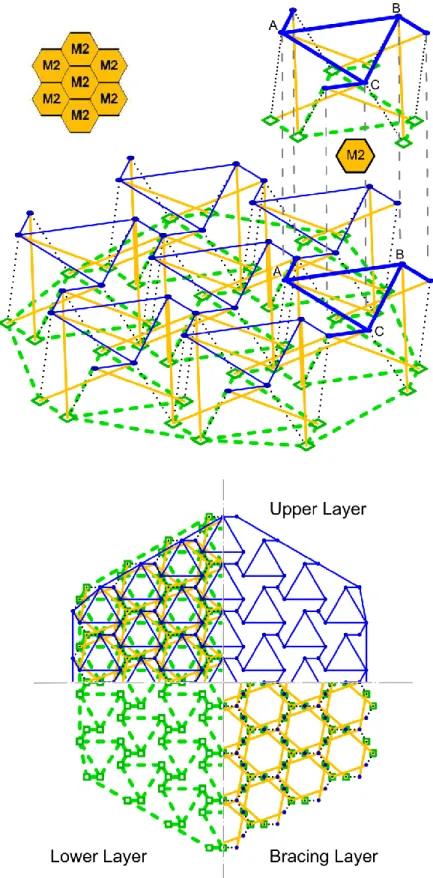
Figure 11. DLTG obtained from Rot-Umbela Manipulation of DLTG 36-Be1-Te1. Plan view and perspective. 2

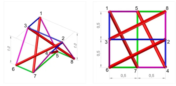
18 1

Figure 12. Perspective and plan view of Quastrut-S 2 3

Independent Modules

Quastrut

As has just been proved in last paragraph, by means of doing a Rot-Umbela Manipulation to DLTG 6

44-Be1-Te1, it is possible to generate two new shapes inside the original grid. These subsystems, 7

when isolated, produce two innovative module configurations. Because they are composed of 8

groups of four struts, we will call them Quastrut (Figure 12). As was shown in precedent figures, 9

there are two ways of connecting the cables of the layers: forming an S-shape, with three 10

stretches forming 90º between them (Figure 12) or forming a Z-shape, with three stretches 11

forming 45º between them (Figure 13). At the moment of their discovery, according to the 12

knowledge of the authors, they were totally novel tensegrity structures. However, thanks to 13

information provided by Dr. Simon D. Guest (personal correspondence) it can be stated that a 14

figure similar to the Quastrut-S was previously illustrated by Grünbaum and Shephard (1975). The 15

image No. 19 of those “Lectures on lost mathematics” shows a plan view of an analogous 16

19

structure, with the same topology but different geometry; however, in those lectures there are 1

not further comments about it. 2

3

Figure 13. Perspective and plan view of Quastrut-Z 4

5

Both modules are chiral or enantiomorphic, i.e. they are non-superimposable on their mirror 6

images. Thus, a dextrorse module (right-handed) and sinistrorse module (left-handed) of each one 7

of them exists. Henceforth, when no reference is made, we will be speaking about the dextrorse 8

module. 9

At this point, we are going to focus on the S-shape configuration, which will be baptized as 10

Quastrut-S, leaving the Z-shape module, which will be called Quastrut-Z, for being studied in 11

following sections along with some other variations. The Quastrut-S is composed of four struts, 12

three bottom wires, three top wires and four diagonal cables, whose shape is square from a plan 13

view, rectangular (depending on the height of the grid) from an elevation view and trapezoidal 14

from a side view. As can be verified in the comparison made in Figure 14, it is similar to a 15

tensegrity module of Half-Cuboctahedron (pyramidal 4-strut module, different to the 16

20

“Quadruplex”, which is the prismatic 4-strut configuration), studied originally by Motro (1987). 1

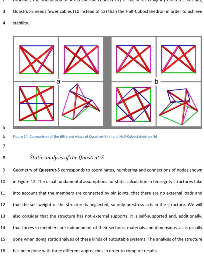
However, the orientation of struts and the connectivity of the wires is slightly different. Besides, 2

Quastrut-S needs fewer cables (10 instead of 12) than the Half-Cuboctahedron in order to achieve 3

stability. 4

5

Figure 14. Comparison of the different views of Quastrut-S (a) and Half-Cuboctahedron (b) 6

7

Static analysis of the Quastrut-S

8

Geometry of Quastrut-S corresponds to coordinates, numbering and connections of nodes shown 9

in Figure 12. The usual fundamental assumptions for static calculation in tensegrity structures take 10

into account that the members are connected by pin joints, that there are no external loads and 11

that the self-weight of the structure is neglected, so only prestress acts in the structure. We will 12

also consider that the structure has not external supports, it is self-supported and, additionally, 13

that forces in members are independent of their sections, materials and dimensions, as is usually 14

done when doing static analysis of these kinds of autostable systems. The analysis of the structure 15

has been done with three different approaches in order to compare results. 16

21

Firstly, a numerical method for calculating the number of mechanisms and states of self-stress by 1

consecutively solving two homogenous linear systems, strongly inspired on the studies on the 2

subject (Pellegrino and Calladine 1986; Pellegrino 1993) and the numerical methods developed by 3

Tran and Lee (2010). By analyzing the Equilibrium Matrix (A), and more specifically its rank, it is 4

possible to obtain the number of mechanisms (m) and states of self-stress (s), defined as: 5

s = null(A) = e – rank(A); [Eq.1]

6

m = dim·b - j – rank(A); [Eq.2]

7

where null(A) is the dimension of null space of the Equilibrium Matrix A, e is the number of 8

members, b is the number of nodes, dim is the dimension (2D or 3D) and j is the number of 9

restrictions of the structure. As tensegrity structures are self-stable, j could be perfectly null (as is 10

our case) in such a way that the total number of mechanisms would also include the rigid body 11

motions (six in 3D, three in 2D). 12

The two linear homogeneous systems of self-equilibrium equations are defined by: 13

A·q = f= 0; [Eq.3]

14

D·[x y z] = 0 [Eq.4]

15

where q is the force density vector, in which each component is the ratio of the normal effort over 16

the length of element (known as force density or self-stressed coefficient), f is the vector of 17

external forces (that we have considered zero) x, y, z are the vectors of nodal coordinates and D is 18

the Force Density Matrix. If the following three conditions are satisfied, then the d-dimensional 19

tensegrity structure is stable independently of the selection of materials and the level of self-20

stresses (Zhang and Ohsaki 2007): 21

22

1) The force density matrix D has the minimum rank deficiency (dim + 1). 1

2) D is positive semidefinite. 2

3) Rank of the geometry matrix G is dim·(dim + 1)/2 (in 3D, rank(G)=6). 3

A second step in the analysis is the calculation of the state of self-stress was carried out by means 4

of, a real time implementation (a software application) of a discrete element method (mass-spring 5

systems) (Averseng et al. 2012). This is an explicit dynamic nonlinear analysis, although for our 6

purpose it was used as a versatile method for the design and static analysis of tensegrity systems. 7

Because these systems are assimilated to discrete mass-spring systems, the simulation of their 8

dynamic behavior can be implemented efficiently. Associating the calculations (based on C++ GLUT 9

library) with an interactive visualization interface (OpenGL), it becomes possible to create and 10

modify structures in real time, with a direct feedback on their behaviour (Fig. 15). This graphical 11

simulation program developed by Averseng, named ToyGL (version dec. 2009), is the tool used by 12

the present authors to work out the form-finding and calculations of the structures presented in 13

this work. It permits traditional and new structures to be designed and, once defined, interact in 14

real time with them by changing with the mouse and the keyboard the length of their members, 15

weights, supports, position of the nodes, etc. 16

23 1

Figure 15. Screen capture of Quastrut-S in software ToyGL (by Julien Averseng) 2

3

Their dynamics are determined using an explicit fourth order Runge-Kutta (RK4) time integration 4

scheme. The system is defined kinetically by its dynamic state X(t), which is the sets of the 5

positions and the speeds of the nodes at a given time t, defined by: 6

[Eq.5] 7

During the RK4 processing, the dynamic state X(t) is successively computed from the combination 8

of first-order derivatives of the state of the system X’(t) = f(X,t), which actually rely on the 9

determination of forces to the nodes, defined by: 10

[Eq.6] 11

24

And finally, the third step was developed using a modified dynamic relaxation (DR) algorithm 1

applied to clustered tensegrity structures (Bel Hadj Ali et al., 2011). This method, implemented in a 2

Matlab code and modified slightly by the present authors with the open license software Octave 3

(version 3.6.1), was used to assess and define the real movements of the nodes of the structure 4

when the state of self-stressed was applied to it. Doing so, it was possible to verify that the force 5

density vectors obtained with the classical approach of Eq.3, were correct and precise. The 6

algorithm also calculates the modification of the coordinates of the nodes, lengths and forces of all 7

members and some other performances that were not fully used for this purpose, like the effect of 8

continuous cables on the structural behavior (which reduces the number of independent states of 9

self-stress and the number of internal mechanisms). 10

The general DR method (Bel Hadj Ali et al., 2011) implements static equilibrium equations (Eq. 7) 11

by means of considering inertial (M) and damping (C) expressions (Eq. 8): 12

Fint ( ) = Fext [Eq.7]

13

Fint ( ) + {M· + C· } = Fext [Eq.8]

14

where Fint and Fext are the vectors of internal and external forces respectively, u and v are the 15

vectors of nodal displacements and velocities, and finally M and C are the mass and damping 16

matrix. Eq. 8 could also be expressed as 17

M· t + C· t = Rt [Eq.9]

18

where R is the residual force vector, obtained as the difference between external and internal 19

forces at any time t. From this point, DR basic equations are obtained by following central 20

difference approximations (Eq.10), used for temporal derivatives, and then by re-arranging Eq.9 in 21

form of Eq.11: 22

25

; [Eq.10]

1

[Eq.11] 2

where subscript i,x means ith node, direction x (respectively, for directions y and z). Finally, 3

displacements at time (t + Δt) are obtained from velocities: 4

[Eq.12] 5

Calculations, carried on with the first methodology, prove the existence of five mechanisms (m=5) 6

and just one state of self-stress (s=1). The module is not only stable, but also super stable, as it is 7

stated by the fact that the force density matrix is positive definite (Connelly 1999). The only 8

feasible self-stress mode is the one where tensions in bars, top/bottom cables and diagonal cables 9

are -3, 2 and 2.236 respectively (Table 1). Comparison of the results of the state of self-stress of 10

the first method with the second and third ones diverge in less than 0,004% and 0,01% 11

respectively. 12

13

Type of element Quastrut-S Rigid Quastrut-Z Rigid Quastrut-S-Z Octag. Quastrut-S-Z

Struts -3.00000 -1.34164 -1.34164 -2.15045 / -1.31189

Additional Struts -1.26491 -1.26491

Bottom original Wires 2.00000 1.34164 1.34164 1.09626 / 1.05606 Top original Wires 2.00000 1.34164 0.89443 1.09626 / 1.05606

Diagonal Wires 2.23607 1.00000 1.00000 1.67552 / 1.00000

Additional Bottom Wires 1.00000 1.00000

Additional Top Wires 1.00000

Short Elem./Long Elem. Table 1. Initial state of self-stress depending on the type of elements of the different Quastruts.

14 15

Those five internal mechanisms correspond to the relative displacements of the four nodes where 16

just two wires concur, and the rotation between bases superior and inferior. In fact, every time 17

26

that additional wires are added to the bases of the module between those nodes (1-2, 3-4, 5-6 and 1

7-8 of Figure 16), the number of mechanisms are decreased continuously until having just the 2

typical one (relative rotation of the bases). Paradoxically, in this Rigid Quastrut-S module of Figure 3

16, the state of self-stress is the same as in the flexible or original one, because the additional 4

cables are barely taking any tension. 5

6

Figure 16. Rigid Quastrut-S with four cables (1-2, 3-4, 5-6 and 7-8) added to the Quastrut-S 7

8

Figure 17. Perspective and plan view of Sixstrut 9

27 1

Sixstrut

2

Using the same procedure that has been applied for obtaining the Quastrut, but working with a 3

different grid, (i.e. applying Rot-Umbela Manipulation to DLTG 36_{-Be1-Te1), it is possible to} 4

generate another new tensegrity module inside the original grid. This novel structure, which 5

analogously to Quastrut will be called Sixstrut because of the number of bars that it composes, is 6

shown in Figure 17. 7

Analogously to Quastrut-S, this tensegrity module is super stable and has just one state of self-8

stress (s=1). Its six mechanisms (m=6) correspond to the inextensional displacements of the six 9

nodes where just two wires concur. 10

Octastrut, Decastrut, etc.

11

The topology and geometry of the Quastrut and Sixstrut modules and especially the connections 12

of the bars inside the prism, are of particular interest. 13

14

Figure 18. Disposition of nodes of Quastrut-S 15

28

Let’s take as an example the Quastrut-S of Figure 18, naming its vertices as A, B, C, being those of 1

the top layer At, Bt, Ct... and those of the bottom layer Ab, Bb, Cb… Thus, the edges of the prism 2

are Ab-Bb-Cb, Cb-Db-Eb, Eb-Fb-Gb, etc. In Quastrut module, the struts go from, for instance, the 3

vertex Ab of an edge (Ab-Bb-Cb) of one base of the prism (e.g. bottom layer) to the midpoint (Dt) 4

of an adjacent edge Ct-Dt-Et (opposite to the vertex of origin Ab), of the other base of the prim 5

(e.g. top layer). This is shown in Figure 18. 6

Inspired by the characteristic topology of the Quastrut modules, it is also possible to define some 7

new configurations with different prisms whose bases have an even number of sides, i.e., 8

hexagons, octagons, decagons, etc. The new structures will be named following the same pattern 9

of the Quastrut, that is, Sixstrut (already obtained by Rot-Umbela Manipulation of DLTG 36 -Be1-10

Te1), Octastrut, Decastrut, etc. 11

It should be pointed out, that the higher the number of struts of these kinds of structures, the 12

more instable they are, due to the increasing number of mechanisms arising in the system. For 13

avoiding this, it is possible to include additional wires in the boundary of the prisms in order to 14

stiffen them accordingly. This would be considered the rigid variation of those modules. 15

Besides, because of the way of defining the geometry of these modules, when the number of sides 16

of the bases is increased, the struts get closer and it is easier that they have interferences and 17

touch each other. 18

As an example, Figure 19 shows an Octastrut (s=1, m=10) where, even if the struts do not collide, 19

at least they are very close. Additional diagonal wires have been introduced at the periphery in 20

order to assure its stability. 21

29 1

Figure 19. Plan view and perspective of Octastrut 2

However, differently to what could be thought, it is not possible to obtain the Octastrut from the 3

application of Rot-Umbela Manipulation to DLTG [4,8,8]-Be1-Te1 (Raducanu’s “4 ways grid”, 4

composed by expanders V44, similar to expanders V22 but with four struts at each vertex, instead 5

of two), which generates a different grid but not containing the Octastrut. Following the same 6

rules than in precedent cases, if we manipulate that grid using: 7

 natural umbela valence: u = v = n = 4 (n being the number of struts concurring at each 8

vertex) in both upper and lower nodes; 9

 amplitude: a = L · /2 = L · /2 = L (L being the length of the cables of top and bottom 10

layers) 11

 rotation: r = 270° / n = 67,5° 12

we cannot obtain a new DLTG of class k=n=4. This is due to the fact that in precedent cases we 13

were parting from a tessellation with the same polygons that we have in the Quastrut (squares) 14

and in the Sixstrut (hexagons), but in this case we have again a mosaic of squares while the 15

polygon at the bases of the module is an octagon. 16

30 1

Figure 20. A prototype of a Quastrut-S built with wooden dowels and elastic stripes, in (a) folded position and (b) 2

unfolded position. 3

31

Advantages of the new modules

1

Advantages of the Quastrut-S.

2

The Quastrut has several advantages over other 4-bar tensegrity modules. First of all, the need of 3

fewer elements (10 elements in tension instead of 12) provides more lightness, easier construction 4

assembly and more sense of transparency. Total length of members of a H-C of dimensions 1x1x1 5

units (unit model) is 17,3 units, while in a Quastrut with the same dimensions is 14,5 units (16% 6

lower). Besides, all the modules of the family are characterized for having some nodes with just 7

two wires meeting at them, which simplifies the configuration of the nodes (and thus their costs) 8

and makes any type of deployment of the module easier. A Quastrut-S in a folded and unfolded 9

position is shown in Figure 20, and even if it cannot be appreciated in pictures, release of the 10

element that fixes the module in that flat configuration makes the module come back to its 11

original unfolded shape automatically thanks to the elastic behavior of the tendons. 12

Additionally, as it can be stated in Figure 14, the Half-Cuboctahedron module and some other 4-13

bar tensegrity prisms are characterized for having a twist angle of 45º between the upper and 14

lower polygons of the prism. This fact means that the projection of the grid of wires of the upper 15

layer is not parallel or perpendicular to the wires of the lower layer, not giving, in plan view, the 16

same feeling of order and symmetry as the Quastrut does. 17

Conventional 4-bar tensegrity prisms have a rotational symmetry of 90º, i.e. the modules have 18

exactly the same configuration when rotated 90º about their vertical center axis. However, 19

rotational symmetry of Quastrut is 180º, so when rotated 90º the alignment is not the same, 20

which is very helpful when conforming different DLTGs, as will be seen in next sections of this 21

work. Finally, distribution of stresses is more homogeneous in Quastrut-S, as can be stated in 22

Figure 21. 23

32 1

Figure 21. Comparison of distribution of stresses between Half-Cuboctahedron and Quastrut-S. 2

3

Advantages of the Sixstrut.

4

The Sixstrut has also some advantages over other 6-bar tensegrity prisms. The total length of 5

members of a prism composed by 6 bars, with polygonal bases made of hexagons of side 1 unit 6

and height of the prism also 1 unit is 32,5 units, while in a Sixstrut with the same dimensions is 7

28,6 units (12% lower). Moreover, length of the six members under compression is also much 8

lower (17%), which helps the structure even more in terms of volume of elements, lightness and 9

risk of buckling. 10

Sixstrut is also easily foldable thanks to the configuration of the nodes, where in six of them only 11

two wires are concurring (Figure 22). This fact is analogous to the example shown in Figure 20 for 12

the case of the Quastrut-S. 13

33 1

Figure 22. Prototype of Sixstrut built with wooden dowels and elastic stripes. 2

3

Similarly to what happens with 4-bar modules, conventional 6-bar tensegrity prisms have a 4

rotational symmetry of 60º, while rotational symmetry of Sixstrut is 120º, so when rotated 60º the 5

alignment is not the same, which gives more versatility to the design of different types of DLTGs. 6

For the rest of the family (Octastruts, Decastruts, etc.), the conclusions of the analysis are similar 7

to those of Sixstrut. 8

9

Variations of the Quastrut

10

As we have seen above, when applying the Rot-Umbela Manipulation to the original DLTG 44 -Be1-11

Te1, there are two possibilities for doing the connection of the wires on the bases of the modules. 12

34

Z-shape: Quastrut-Z

1

The second variation, obtained in Figure 4.b and already exposed in Figure 13, occurs when 2

horizontal wires form a Z-shape, having the long wires in the diagonal of the square in plan view. 3

Coordinates are the same as those of Quastrut-S, but the topology is different and corresponds to 4

the connections shown in Figure 23. However, this original configuration, also called Quastrut-Z, is 5

not stable by itself, having four internal mechanisms (m=4) and no state of self-stress (s=0) 6

capable to stiffen the structure. Thus, it cannot be considered a tensegrity structure. 7

8

Figure 23. Quastrut-Z and disposition of the four nodes (No. 2, 3, 5 and 7, marked with circles) with just two cables 9

concurring at them 10

11

This is due to the fact that, in this structure, there are four nodes (No. 2, 3, 5 and 7, marked with 12

circles in Figure 23) at which are concurring just two cables along with the strut. In order to be in 13

equilibrium, the resultant of the three lines of forces must be zero, thus, the three elements must 14

be in the same plane. As it is noted in Figure 23, it does not happen in the Z-shape configuration, 15

and the system must modify the position of its nodes in order to achieve that equilibrium 16

condition. 17

35

There are some other examples, apart from the Quastrut-S, Sixstrut and Octastrut, of these kinds 1

of structures where there are only one strut and two cables concurring at a node, maintaining 2

perfectly the stability of the system. For instance, the Skylon Structure Sculpture (Francis 1980), 3

many of Marcelo Pars’ tensegrity fans (Pars 2008) and the Stella Octangula (Emmerich 1988). 4

In order to keep the original shape of the Quastrut-Z, it is necessary to add extra wires, especially 5

at the nodes where there are two and not three cables concurring. The system illustrated in Figure 6

24, the Rigid Quastrut-Z, has additional parallel cables in diagonal in both layers (1-2, 3-4, 5-6 and 7

7-8). Such a structure has one mechanism (m=1) and one state of self-stress (s=1), which is shown 8

in Table 1. It can be noted that there are six negative stresses (corresponding to elements under 9

compression), two more than the four struts of the initial system. This is because the two 10

diagonals of the Z-shape of the bases (1-4 and 6-8), one in each layer, must be under compression. 11

In such a way, it is possible to keep the stability as a whole. Because there are struts in contact, the 12

structure switches to class k=2, creating two enchained set of struts doing zigzag between 13

opposite vertices. 14

15

Figure 24. Rigid Quastrut-Z with four cables added to the Quastrut-Z on top layer (5-6, 7-8) and bottom layer (1-2, 3-16

4). The original wires 1-4 and 6-8 became struts in order to give stability to the structure. 17

36

S-Z-shape: Quastrut-S-Z

1

Moreover, there is a third variation, the S-Z-shape, created when both configurations exposed 2

above are mixed together. In this case, the bottom wires form a Z-shape while the top wires form 3

an S-shape (or vice versa). In this module, the position of its nodes change sensitively in order to 4

reach the equilibrium conditions mentioned in precedent paragraph, which affects mainly the two 5

vertices (No. 5 and 7, which are circled in Figure 25) of the layer with cables having a Z-shape. 6

7

Figure 25. Quastrut-S-Z and disposition of the two nodes (No. 5 and 7 which are circled) with just two cables 8

concurring at them 9

10

One of the feasible conversions from the theoretical shape to a real configuration, without adding 11

extra elements, is the Octagonal Quastrut-S-Z, with coordinates of nodes shown in Figure 26. It is 12

verifiable that the new module acquires an irregular octagonal shape when projected in the 13

horizontal plane. Regular octagonal configuration is impossible due to geometric reasons. The 14

symmetry of the structure would create interferences between the struts. The main condition to 15

obtain the equilibrium is that the two struts where only two wires are concurring (At-Db and Ft-16

Cb), are in the same plane than their contiguous cables. In Figure 26, strut At-Db, for instance, 17

37

must be in the same plane than cables arriving to the vertex At (At-Hb and At-Bt) and arriving to 1

the vertex Db (Db-Cb and Db-Et). 2

3

Figure 26. Perspective and plan view of the Octagonal Quastrut-S-Z and disposition of nodes 4

5

6

Figure 27. Rigid Quastrut-S-Z with 2 cables added to the Quastrut-S-Z 7

38

It is possible to find, in this configuration, five mechanisms (m=5), and one state of self-stress 1

(s=1), which is presented in Table 1 (values are shown depending on the length of the connections: 2

Short Elements / Long Elements). 3

Obviously, as in the case of the Quastrut-Z, it is also possible to fix the original geometry S-Z 4

(shown in Figure 25, having the same coordinates as Quastrut-Z) by means of including extra 5

cables in the base where cables form a Z-shape. The result, shown in Figure 27, is found by 6

switching the diagonal cable in the middle of the base for an extra strut, in order to achieve 7

stability. In this case the structure has three infinitesimal mechanisms (m=3) and only one 8

independent self-stress mode (s=1), exposed in Table 1. 9

DLTG Quastrut

10

The final grid obtained after the application of the Rot-Umbela Manipulation to the DLTG 44 -Be1-11

Te1 was already presented in Figure 6. As has been claimed above, it is the same as considering 12

the juxtaposition of Quastrut-S Dextrorse Modules aligned 0º 13

As can be observed in Figure 6, where a certain state of self-stress has already been applied, the 14

DLTG is stable, even if it looks like there are some wires missing. The designer would like to have 15

the boundaries of the upper and lower layers to be closed, as well as some of the diagonal wires of 16

the periphery. In that case, after the addition of those extra elements at the boundaries, the new 17

grid would be more rigid and stable. Henceforth, these cases will be denominated “Closed” 18

arrangements. In case the addition of extra elements is applied just to the bottom and top layer 19

(horizontal cables), and not to web layer (diagonal cables), they will be called “Semiclosed”, as 20

appears in Figure 28. Moreover, there are some other variations, like the “Rigid” configurations, 21

where extra wires are also included not only in the periphery of the grid, but also in the interior 22

parts of the bottom, top and web layers of the DLTG. 23

39 1

Figure 28. DLTG Quastrut-S No.1s, monogyre (dextrorse modules), rotation 0º, semiclosed configuration. 2

40

Some other Variations of DLTG

1

Emmerich (1988) proposed the generation of many DLTG, composing them with some basic 2

modules and their variations. The French engineer generated the variations by means of using the 3

tensegrity anti-prisms (cylinder-shape simplex modules), anti-pyramids (tensegrity truncated-4

pyramid modules) and interpenetrated modules. It is also possible to do the same with the 5

modules obtained above. 6

As it happens with the tensegrity basic systems studied by Emmerich, our modules are 7

enantiomorphic, so it is possible to use a “monogyre” composition with either dextrorse or 8

sinistrorse modules, or a “racemic” arrangement, i.e. using both dextrorotatory and levorotatory 9

forms of the modules. 10

Besides, the different enantiomers can be rotated, aligning them at 0º, 45º, 60º, 90º, etc. 11

(depending on the geometry of the module), and thus conforming different grids by combining 12

their several variations. 13

As a result, taking the whole list of modules exposed until this point in this paper, it is possible to 14

create a wide range catalogue of different DLTGs attending to the combinations of all of them. For 15

example, some of the different possibilities offered by the juxtaposition of the Quastrut-S are 16

exposed in Table 2. In that chart, additional configurations have been added to the simplest grid, 17

the Quastrut-S monogyre, i.e. SemiClosed, Closed and Rigid grids. The same variations are also 18

applicable to the other grids, but there are not included for simplifying the exposition of the data. 19

Some graphical examples of these potentials are shown in Figure 29, Figure 30 and Figure 31. 20

41 1

Figure 29. DLTG Quastrut-S No.2, monogyre, rotations 0º and 90º, open configuration. 2

42 1

2

Figure 30. DLTG Quastrut-S No.3, racemic, rotation 0º, open configuration. 3

43 1

2

Figure 31. DLTG Quastrut-S No.4, racemic, rotations 0º and 90º, open configuration 3

44

Table 2 also presents some additional information about these grids, like the tensegrity class (k), 1

the number of internal mechanisms (m) and states of self-stress (s) for several square 2

compositions of NxN modules. It is not the intention of the authors to give explanations in full 3

detail about these properties, in order to keep the length of this paper reasonable. Obviously, all 4

the research related to this point will be presented in more detail in further communications. 5

1x1 2x2 3x3 4x4

No. Module Gyre Rotation Variation k s m s m s m s m 1 Quastrut-S Mono 0 Open 2 1 5 4 20 9 33 17 45

1s Quastrut-S Mono 0 SemiClosed 2 1 5 5 9 13 17 25 25

1c Quastrut-S Mono 0 Closed 2 1 5 5 5 13 9 25 13

1r Quastrut-S Mono 0 Rigid 2 1 5 5 1 17 1 37 1

2 Quastrut-S Mono 0-90 Open 4 1 5 4 17 9 33 16 53 3 Quastrut-S Racemic 0 Open 4 1 5 4 13 9 21 16 29 4 Quastrut-S Racemic 0-90 Open (*) 2 1 5 2 27 4 56 8 93

(*) Some diagonal wires changed for vertical wires to avoid intersections between them. Table 2. Some of the variations of the DLTG Quastrut-S and their characteristics

6 7

Analogously, it is straightforward to generate some other DLTGs taking as a point of depart 8

tessellations created by combinations of polygons with the same number of edges than the 9

modules originated above. Another example is presented in Table 3 and Figure 32, with some 10

possibilities for grids composed by modules of Sixstruts. Figure 6 would correspond to the DLTG 11

Sixstrut No.1, monogyre, rotation 0º, open configuration. 12

45 1

Figure 32. DLTG Sixstrut No.4s, racemic, rotation 0-60º, semiclosed configuration. 2

46

1M 7M

No. Module Gyre Rotation Variation k s m s m

1 Sixstrut Mono 0 Open 3 1 6 7 28

1s Sixstrut Mono 0 SemiClosed 3 1 6 7 10

1c Sixstrut Mono 0 Closed 3 1 6 7 4

2 Sixstrut Mono 0-60 Open 3 1 6 7 28

3 Sixstrut Racemic 0 Open 2 1 6 7 43

4 Sixstrut Racemic 0-60 Open 3 1 6 7 19

Table 3. Some of the variations of the DLTG Sixstrut and their characteristics. 1

2

Finally, in order to show the combination of different kinds of modules, Table 4 exposes some 3

variations of the DLTG 6-4-3-Strut composed by Quastrut-S (4 sides) and Sixstrut (3 sides), leaving 4

between some of them empty spaces with triangular shape (3 sides). Figure 33 is an illustration of 5

the rigid configuration. The same exercise could be done with many other tessellations (e.g. 4-8-8, 6

3-4-6-4, etc.) 7

7M No. Module Gyre Rotation Variation k s m

1 6-4-3-Strut Mono 0-60 Open 3 7 33

1s 6-4-3-Strut Mono 0-60 SemiClosed 3 7 15

1c 6-4-3-Strut Mono 0-60 Closed 3 7 9

1r 6-4-3-Strut Mono 0-60 Rigid 3 13 1

Table 4. Main variations of the DLTG 6-4-3-Strut and their characteristics 8

47 1

Figure 33. DLTG 6-4-3-Strut No.1r, monogyre, rotations 0º and 60º, rigid configuration. 2

48

Conclusions

1

It has been proved that the use of Rot-Umbela Manipulations applied to DLTG produces some 2

other new and unknown, until now, tensegrity grids. In this paper, these operations have been 3

applied to grids composed by Expanders V22 and V33. 4

A closed observation of the new grids permits a new kind of tensegrity modules to be obtained, 5

baptized as Quastruts and Sixstruts, integrated in the novel grids. The analysis of these modules, 6

and some of their variations, leads to the conclusion that they belong to a new family of tensegrity 7

systems based on rotational symmetry. Thus, it could be concluded that the use of Rot-Umbela 8

Manipulations to conventional or tensegrity structures may lead to the discovery of innovative 9

tensegrity systems unidentified at the present time. 10

Finally, it has also been proved that the combination of these new tensegrity structures can 11

produce new DLTG attending to their different variations, ways of composing them and 12

methodologies for stiffening them. 13

14

Further research

15

This paper exposes a particular methodology for obtaining innovative DLTGs. It also deals with the 16

static analysis of the new modules and the grids composed with them, albeit in not much detail. 17

Thus, the next steps lead to a more complete and full research on the stability, rigidity, resistance 18

and deformation of these novel structures and some other variations derived from the 19

methodologies exposed above. Analysis of their mechanisms and states of self-stress will help to 20

understand their structural characteristics better. 21

49

Stiffness of tensegrity structures depends on their geometry, connectivity and material properties, 1

as well as on their level of prestress (Guest 2011). Therefore, special attention must be applied to 2

the self-stress of the novel modules and the grids derived from them. 3

Further analysis will be done in order to compare the behavior between these new grids (e.g. 4

DLTG Quastrut Vs. DLTG Sixstrut), their variations (e.g. monogyre Vs. racemic; 0º Vs. 90º) and their 5

configurations (e.g. open Vs. closed). Besides, it would also be interesting to compare them with 6

other grids already existing and well known by the tensegrity researchers. 7

8

Acknowledgments

9

The authors are grateful to Landolf Rhode-Barbarigos and Prof. Smith, from IMAC at EPFL for their 10

generosity sharing their useful tools for the analysis of the structures (Bel Hadj Ali et al. 2011), as 11

well as to Dr. Julien Averseng, from LMGC at University of Montpellier, for the valuable help 12

contributed by his software (Averseng et al. 2012). Comments on the origins of the Quastrut, by 13

Dr. Simon Guest, were also very appreciated. 14

The corresponding author would also like to thank the Basque Delegation of the Spanish College of 15

Civil Engineers for their support during the time while this research was carried out. 16

17

References

18

Averseng, J., Quirant, J., and Dubé, J.-F. (2012). “Interactive design and dynamic analysis of 19

tensegrity systems.” ). International Journal of Space Structures, 27(Special Issue 2-3). 20

Bel Hadj Ali, N., Rhode-Barbarigos, L., and Smith, I. (2011). “Analysis of clustered tensegrity 21

structures using a modified dynamic relaxation algorithm.” International Journal of Solids and 22

Structures, 48(5), 637–647. 23

50

Connelly, R. (1999). “Tensegrity Structures: Why are They Stable?” Rigidity theory and 1

applications. MF Thorpe and PM Duxbury (Eds.), Kluwer/Plenum Publishers, 47–54. 2

Dalilsafei, S., and Tibert, G. (2012). “Design And Form-Finding Analysis Of Tensegrity Power Lines.” 3

International Journal of Space Structures, 27(Special Issue 2-3). 4

Emmerich, D. G. (1964). “Structures linéaires autotendants.” French. 5

Emmerich, D. G. (1988). Structures tendues et autotendantes. Ecole d’architecture de Paris la 6

Villette, Paris. 7

Francis, A. J. (1980). Introducing structures: a textbook for students of civil and structural 8

engineering, building, and architecture. Pergamon Press, Oxford. 9

Gancedo Lamadrid, E., José Manuel Álvarez Gómez, Jesús Suárez González, and Javier Vega 10

Menéndez. (2004). “A New Method to Obtain and Define Regular Polyhedra.” Geometriae 11

Dedicata, 106(1), 43–49. 12

Gomez-Jauregui, V. (2010). Tensegrity structures and their application to architecture. 13

Books&Science, Universidad de Cantabria. Servicio de Publicaciones, Santander. 14

Gomez-Jauregui, V. (2012). “Mallas tensegríticas de doble capa y manipulaciones de Rot-Umbela.” 15

Informes de la Construcción. 16

Gomez-Jauregui, V., Arias, R., Otero, C., and Manchado, C. (2012). “Novel technique for obtaining 17

double-layer tensegrity grids.” International Journal of Space Structures, 27(Special Issue 2-3), 18

155–166. 19

Gomez-Jauregui, V., Otero, C., Arias, R., and Manchado, C. (2011). “New configurations for double-20

layer tensegrity grids.” Structural Engineers World Congress 2011, Como (Italy). 21

Gomez-Jauregui, V., Otero, C., Arias, R., and Manchado, C. (2012). “Generation and nomenclature 22

of tessellations and double-layer grids.” Journal of Structural Engineering-ASCE, (July 2012). 23

Grünbaum, B., and Shephard, G. (1975). “Lectures in lost mathematics, mimeographed notes.” 24

Univ. of Washington. 25

Guest, S. (2011). “The stiffness of tensegrity structures.” IMA Journal of Applied Mathematics, 26

76(1), 57. 27

Hanaor, A. (1991). “Double-layer tensegrity grids: static load response. II: Experimental study.” 28

Journal of Structural Engineering-ASCE, 117(6), 1675–1684. 29

Knight, B., Duffy, J., Crane, C., and Rooney, J. (2000). “Innovative deployable antenna 30

developments using tensegrity design.” Collection of Technical Papers - 31

AIAA/ASME/ASCE/AHS/ASC Structures, Structural Dynamics and Materials Conference, AIAA, 32

Atlanta, GA, USA, 984–994. 33

51

Kono, Y., and Kunieda, H. (1996). “Tensegrity grids transformed from double-layer space grids.” 1

Stuttgart, 293–300. 2

Mitsos, I., Guest, S., Winslow, P., and Martin, B. (2011). “Experimental investigation of a double 3

layer ‘Tensegrity’ space frame.” London. 4

Motro, R. (1987). “Tensegrity systems for double layer space structures.” Proceedings of 5

International Conference on the Design and Construction of Non-conventional Structures, Civil- 6

Comp Press., Edinburgh, Scotland. 7

Motro, R. (2003). Tensegrity : Structural systems for the future. Kogan Page Science, London (UK). 8

Panigrahi, R., Gupta, A., and Bhalla, S. (2009). “Dismountable steel tensegrity grids as alternate 9

roof structures.” Steel and Composite Structures, 9(3), 239–253. 10

Pars, M. (2008). “Tensegriteit.” <http://www.tensegriteit.nl/> (Jan. 10, 2009). 11

Pellegrino, S. (1993). “Structural computations with the singular value decomposition of the 12

equilibrium matrix.” International Journal of Solids and Structures, 30(21), 3025–3035. 13

Pellegrino, S., and Calladine, C. R. (1986). “Matrix analysis of statically and kinematically 14

indeterminate frameworks.” International Journal of Solids and Structures, 22(4), 409–428. 15

Raducanu, V. (2001). “Architecture et système constructif: Case de systémes de tenségrité.” PhD, 16

Université de Montpellier II, Montpellier. 17

Rhode-Barbarigos, L., Hadj Ali, N. B., Motro, R., and Smith, I. F. C. (2010). “Designing tensegrity 18

modules for pedestrian bridges.” Engineering Structures, 32(4), 1158–1167. 19

Skelton, R. E., Adhikari,, R., and Helton, J. W. (1998). “Mechanics of Tensegrity Beams.” UCSD, 20

Structural Systems & Contr. Lab., Rep. No. 1998-1. 21

Stucchi, S., Micheletti, A., Santangelo, F., and Totaro, A. (2006). “Tensegrity Units for a Movable 22

Settlement.” Proceedings of Adaptables, Eindhoven, 95–99. 23

Tran, H. C., and Lee, J. (2010). “Initial self-stress design of tensegrity grid structures.” Computers 24

and Structures, 88(9-10), 558–566. 25

Zhang, J. Y., and Ohsaki, M. (2007). “Stability conditions for tensegrity structures.” International 26

Journal of Solids and Structures, 44(11-12), 3875–3886. 27

28 29