Income and wealth distribution with physical and human capital accumulation : extending the Uzawa Lucas model to a heterogeneous households economy

Texto completo

(1)Vol. 50 No. 2 (NOV, 2013), 257–287. Income and Wealth Distribution with Physical and Human Capital Accumulation: EXTENDING THE UZAWALUCAS MODEL TO A HETEROGENEOUS HOUSEHOLDS ECONOMY* Wei-Bin Zhang** This paper proposes a dynamic economic model with wealth accumulation and human capital accumulation with endogenous education. In addition to learning by education like in the Uzawa-Lucas model, we also consider Arrow’s learning by producing and Zhang’s learning by consuming (creative learning) in the human capital accumulation equation. We simulate the model to demonstrate the existence of equilibrium points and motion of the dynamic system. We also examine how ef fects of changes in the propensity to receive education, the population, the propensity to save, and the education sector’s total productivity will alter the paths of the economic dynamics. JEL classification: O41, I2 Keywords: learning by producing, learning by consuming, learning by education, wealth and income distribution, heterogeneous households. 1.. Introduction. Dynamic interdependence between economic growth and human capital is currently a central topic in economic theory and empirical research. It has become evident that capital accumulation is not suf ficient for explaining why countries grow dif ferently, as posited by neoclassical growth theory. As Easterlin (1981) observed, in 1850 there were few people outside northwestern Europe and North America who had any formal education, and the spread of formal schooling seems to have preceded the beginning of modern economic growth. In modern economies, human capital is a key determinant of economic growth1 and there have been many studies on the dynamic interdependence. * The author is grateful to the anonymous referee and editor Felipe Zurita for their constructive comments and suggestions, and acknowledges financial support from the Grants-in-Aid for Scientific Research (C), Project No. 25380246, Japan Society for the Promotion of Science. ** Professor, Ritsumeikan Asia Pacific University, 1-1 Jumonjibaru, Beppu-Shi, Oita-ken, 874-8577, Japan. Tel: 0977-78-1010; email: [email protected]. 1. For instance, see Hanushek and Kimko (2000), Barro (2001), Krueger and Lindahl (2001), and Castelló-Climent and Hidalgo-Cabrillana (2012).. doi 10.7764/LAJE.50.2.257.

(2) 258. LATIN AMERICAN JOURNAL OF ECONOMICS | Vol. 50 No. 2 (Nov, 2013), 257–287. between education and economic growth in literature of economic theory and empirical economic studies. Estimating the impact of education on earnings has been the focus of numerous empirical studies since Mincer (1974) published his seminal work. He finds that for white males not working on farms, an additional year of education raises income by about 7%. Other studies (Tilak, 1989) have shown that the spread of education can substantially reduce inequality within countries. Could et al. (2001) build a model to provide insights into the evolution of wage inequality within and between industries and education groups in the recent decades. The model shows that increasing randomness is the primary source of inequality growth among uneducated workers, but inequality growth among educated workers is determined more by changes in composition and return to ability (which is closely related to education). Tselios (2008) studies the relationship between income and educational inequalities in the regions of the European Union, using the European Community Household Panel data survey for 94 regions over the period 1995-2000. The research findings suggest a positive relationship between income and educational inequalities. Fleisher et al. (2011) examine the role of education in worker productivity and firms’ total factor productivity on the basis of firm-level data from China. The study shows that an additional year of schooling raises marginal product by 30.1 percent, and the CEO’s education increases TFP for foreign-invested firms. The return is also closely related to ownership. For instance, the ef fect of schooling on productivity is highest in foreign-invested firms. One significant conclusion is that market mechanisms contribute to more ef ficient use of human capital within firms. Zhu (2011) studies individual heterogeneity in returns to education in China from 19952002, finding heterogeneous ef fects both within and between gender groups. In Zhu’s study, heterogeneity in schooling returns falls from 1995 to 2002 for both genders in urban China, although their rates of education return have increased substantially. One reason for the narrowing heterogeneity is a better-functioning and increasingly integrated urban labor market in China. The literature on endogenous knowledge and economic growth has expanded since Romer (1986) re-examined issues of endogenous technological change and economic growth in his 1986 paper.2 But it 2. See Lucas (1988), Grossman and Helpman (1991), and Aghion and Howitt (1998)..

(3) Wei-Bin Zhang | THE UZAWA-LUCAS MODEL WITH HETEROGENEOUS HOUSEHOLDS. 259. is the work of Lucas (1988) that has created substantial interest in formal modeling of education and economic growth among economists. The first formal dynamic growth model with education was actually proposed by Uzawa (1965). In the Uzawa-Lucas model and many of its extensions and generalizations, it is implicitly assumed that all skills and human capital are developed by formal schooling. However, much of human capital may be accumulated through family and other social and economic activities. For instance, the human capital of a graduate student from a wealthy family in the U.S. may be quite dif ferent from the human capital of a graduate student from a middle-class family in India. By ignoring non-school factors, we may misunderstand the role of formal education in economic development. Another issue is described by Chen and Chevalier (2008): “Making and exploiting an investment in human capital requires individuals to sacrifice not only consumption, but also leisure. When estimating the returns to education, existing studies typically weigh the monetary costs of schooling (tuition and forgone wages) against increased wages, neglecting the associated labor/leisure tradeof f.” The purpose of this study is to introduce other sources of learning into the Uzawa-Lucas two-sector growth model. Another key purpose of this study is to introduce heterogeneous households into the two-sector growth model with education. Dif ferent households have dif ferent propensities to save and obtain education, as well as dif ferent abilities to absorb knowledge and increase human capital through education, learning by doing and learning by consuming. Most of the extensions and generalizations of the Uzawa-Lucas model are limited to a single representative household. However, there are models of endogenous human capital with heterogeneous households. For instance, Galor and Zeira (1993) propose a model to study the relationship between growth and inequality with human capital as the driving force of economic growth. A main conclusion of their study is that in the presence of credit constraints on human capital investments, high initial inequality may reduce long-run growth, while redistribution may increase the growth rate. Maoz and Moav (1999) build a similar model and show that the impact of income redistribution is situation-dependent. In another model by Galor and Moav (2004), it is demonstrated that in the early stage of modern economic development, high inequality encourages growth as the rich have a higher propensity to save, whereas at later stages high inequality may discourage growth as human capital becomes.

(4) 260. LATIN AMERICAN JOURNAL OF ECONOMICS | Vol. 50 No. 2 (Nov, 2013), 257–287. increasingly important and high inequality may be an impediment to human capital accumulation. Fender and Wang (2003) build an overlapping-generations model with endogenous education choice with and without credit constraints. In their model, credit constraints are associated with lower education and a lower rate of interest. Laitner (2000) examines the dynamics of earnings within education groups and overall productivity using a model with endogenous human capital and a distribution of natural abilities. In a model of education where the distribution of abilities is the source of heterogeneity, Cardak (2004) shows that private education results in higher incomes and less income inequality than the public education model. Erosa et al. (2010) build a model of endogenous human capital accumulation with education to explain the variation in per-capita income across countries. Further literature can be found in the studies cited. A main deviation of our approach from the previous models is that we derive demand for education in an alternative to the typical Ramsey approach. This allows us to explicitly derive the dif ferential equations of the economic system and simulate transition processes. Our model is built on the three main growth models–Solow’s one-sector growth model, Arrow’s learning-by-doing model, and the Uzawa-Lucas growth model with education–in the growth literature. The main mechanisms of economic growth in these three models are integrated into a single framework with heterogeneous households. Our model is also based on the growth model with heterogeneous groups by Zhang (2009). In Zhang’s model, human capital is fixed. The synthesis of the three growth models within a single framework is still analytically tractable because we propose an alternative approach to consumer behavior. The paper is organized as follows. Section 2 introduces the basic model of wealth accumulation and human capital accumulation. Section 3 examines the dynamic properties of the model and simulates the model with three types of households. Section 4 contains our comparative dynamic analysis with regard to certain parameters and Section 5 contains concluding remarks.. 2.. The basic model. In our model, the economy has one production sector and one education sector. Most aspects of the production sector are similar to the standard.

(5) Wei-Bin Zhang | THE UZAWA-LUCAS MODEL WITH HETEROGENEOUS HOUSEHOLDS. 261. one-sector growth model.3 It is assumed that there is only one (durable) good in the economy under consideration. Households own assets in the economy and distribute their incomes to consume and save. Firms use inputs such as labor with varied levels of human capital, different kinds of capital, knowledge and natural resources to produce material goods or services. Exchanges take place in perfectly competitive markets. Factor markets work well; factors are inelastically supplied and the available factors are fully utilized at every moment. Saving is undertaken only by households. All firm earnings are distributed in the form of payments to factors of production, labor, managerial skill and capital ownership. Each – group has a fixed population, Nj , (j = 1,…,J ). Let prices be measured in terms of the commodity and the price of the commodity be unitary. We denote wage and interest rates by wj(t) and r(t) respectively. We use Hj(t) to stand for group j’s level of human capital. The total capital stock K(t) is allocated between the two sectors. We use Ni(t) and Ki(t) to stand for the labor force and capital stocks employed by the production sector, and Ne(t) and Ke(t) for the labor force and capital stocks employed by the education sector. We use Tj(t) and Tje(t) to stand for, respectively, the work time and study time of a typical worker in group j. As full employment of labor and capital is assumed, we have: Ki(t) + Ke(t) = K(t),. (1). Ni(t) + Ne(t) = N(t). Where N(t) is the total qualified labor supply defined by: N (t ) =. J. m ∑Tj ( t ) H j ( t ) N j .. (2). j. j =1. We rewrite (1) as follows: ni(t)ki(t) + ne(t)ke(t) = k(t),. ni(t) + ne(t) = 1. in which: kj (t ) ≡. K j (t ) N j (t ). , nj (t ) ≡. N j (t ) N (t ). , k (t ) ≡. K (t ) N (t ). , j = i, e .. 3. See Burmeister and Dobell (1970), Azariadis (1993), and Barro and Sala-i-Martin (1995).. (3).

(6) 262. LATIN AMERICAN JOURNAL OF ECONOMICS | Vol. 50 No. 2 (Nov, 2013), 257–287. 2.1. The production sector We assume that production is to combine the labor force Ni(t) and physical capital Ki(t). We use the conventional production function to describe a relationship between inputs and output. The function Fi(t) is specified as: Fi ( t ) = Ai Kiαi ( t ) N iβi ( t ), Ai , αi , βi > 0, αi + βi = 1.. Markets are competitive, so labor and capital earn their marginal products and firms earn zero profit. The rate of interest and wage rate are determined by markets. For any individual firm, r(t) and wj(t) are given at each point in time. The production sector chooses the two variables Ki(t) and Ni(t) to maximize its profit. The marginal conditions are given by: mj. r ( t ) + δk = αi Ai ki−βi ( t ), w j ( t ) = βi Ai H j. ( t )kiα ( t ), i. (4). where δk is the depreciation rate of physical capital.. 2.2. Education sector We assume that the education sector is also characterized by perfect competition. Here, we do not consider any government financial support for education. Students pay the education fee p(t) per unit of time. The education sector pays teachers and capital at market rates. The total educational service is measured by the total education time received by the population. We specify the production function of the education sector as follows: Fe ( t ) = Ae Keαe ( t ) Neβe ( t ), αe , βe > 0, αe + βe = 1,. (5). Where Ae, αe and βe are positive parameters. The marginal conditions for the education sector are: r + δk =. αe p Fe Ke. m. = αe Ae p ke−βe , w j = βe Ae p H j j keαe .. (6).

(7) Wei-Bin Zhang | THE UZAWA-LUCAS MODEL WITH HETEROGENEOUS HOUSEHOLDS. 263. We see that the demand for labor from the education sector increases with the price and level of human capital and decreases with the wage rate.. 2.3. Consumer behavior and wealth dynamics Consumers make decisions about levels of consumption of education, services and commodities as well as how much to save, and family plays a particularly important role in decisions about investment in education. There are dif ferent models for decisions about education in a family. For instance, in Becker (1981), parents and children share a single unified utility function. In Cox (1987), the family is a nexus for transactions–the old lend to their children who repay them with care during old age. There is also a range between these two formulations in which parents place varying amounts of weight on the income, consumption or human capital of their children.4 In this study, we follow Zhang (2007) in modeling choice of education time. The preference over current and future consumption is reflected in the consumer’s preference structure over education, consumption and – saving. Let k j (t) stand for the per-capita wealth of group j. We have – – – kj (t) = Kj (t)/Nj . Per-capita current income from the interest payment – r(t)k j (t) and the wage payment Tj (t)wj (t) is given by: y j ( t ) = r ( t ) k j ( t ) + Tj ( t ) w j ( t ) .. We call yj(t) the current income in the sense that it comes from consumers’ payment for human capital and effort and consumers’ current earnings from wealth ownership. The sum of money that consumers use for consumption, saving, and education are not necessarily equal to temporary income because consumers can sell wealth to pay, for instance, for current consumption if temporary income is not suf ficient for buying food and travelling the country. The total value of wealth – that consumers can sell to purchase goods and save is equal to k j (t). Here, we assume that selling and buying wealth can be conducted instantaneously without any transaction cost. The per-capita disposable income is given by: yˆj ( t ) = y j ( t ) + k j ( t ) = ( 1 + r ( t ) ) k j ( t ) + Tj ( t ) w j ( t ) .. 4. See Behrman et al. (1982), Fernandez and Rogerson (1998), and Banerjee (2004).. (7).

(8) 264. LATIN AMERICAN JOURNAL OF ECONOMICS | Vol. 50 No. 2 (Nov, 2013), 257–287. Disposable income is used for saving, consumption, and education. It – – should be noted that the value kj (t), (i.e., p(t)kj (t) with p(t)=1), in the above equation is a flow variable. Under the assumption that wealth can be sold instantaneously without any transaction cost, we may consider – kj (t) as the amount of income that the consumer obtains at time t by selling all of his wealth. Hence, at time t the consumer has the total income amount ŷj(t) to distribute among saving, consumption and education. In the growth literature, for instance in the Solow model, saving is proportional to current income, yj(t) while in this study saving is chosen by maximizing the utility subject to the budget constraint. At each point in time, a consumer would distribute the total available budget among saving sj(t), consumption of goods cj(t) and education pj(t)Tje(t). The budget constraint is given by: – cj(t) + sj(t) + pj(t)Tje(t) = ŷj(t) = (1 + r(t))kj (t) + Tj(t)wj(t).. (8). The consumer is faced with the following time constraint: Tj (t) + Tj e(t) = T0,. Where T0 is the total available time for work and study. Substituting this function into (8) yields: – cj(t) + sj(t) + (pj(t) + wj(t))Tje(t) = y–j(t) ≡ (1 + r(t))k j (t) + T0wj(t).. (9). We now introduce a utility function for analyzing household behavior. Here, we consider that education has two kinds of returns. As education raises labor productivity, its ef fect is reflected in higher wages. As Lazear (1977: 570) describes: “...education is simply a normal consumption good and that, like all other normal goods, an increase in wealth will produce an increase in the amount of schooling purchased. Increased incomes are associated with higher schooling attainment as the simple result of an income ef fect.” Education also results in direct pleasure, greater knowledge, higher social status and so on.5 The relative importance of these returns may vary across dif ferent types of education with dif ferent individuals. This study introduces education time as a normal good into the utility function. In our model, at each point in time consumers have three variables to choose: level of consumption, level of saving, and education time. 5. See, for instance, Heckman (1976), Lazear (1977), and Malchow-Møller et al. (2011)..

(9) Wei-Bin Zhang | THE UZAWA-LUCAS MODEL WITH HETEROGENEOUS HOUSEHOLDS. 265. We assume that consumers’ utility function is a function of level of goods cj(t), level of saving sj(t), and education level Tje(t) as follows: U (t ) = c. ξj 0. ( t )s λ ( t )Teη ( t ), j0. j0. ξj 0 , λj 0 , η j 0 > 0,. (10). where ζj0 is called the propensity to consume, λj 0 is the propensity to own wealth, and ηj0 is the propensity to obtain education. This utility function is applied to different economic problems. A detailed explanation of the approach and its applications to different problems of economic dynamics are provided in Zhang (2005, 2009). As discussed by Zhang, this utility function overcomes the problem of the Solow model in which household behavior is modeled without micro-economic foundation. Another approach to household behavior in growth theory is the so-called Ramsey approach. In this approach, the household’s preferences are expressed by an instantaneous utility function, u(c(t)) where c(t) is the flow of consumption per person, and a discount rate for utility, denoted by ρ. Assume that each household maximizes utility U as given by: ∞. U =. ∫ u (c ( t )) e−ρt dt , c ( t ) ≥ 0,. t ≥ 0.. 0. The household makes the decision subject to a lifetime budget constraint. This type of utility formulation means that the household’s utility at time 0 is a weighted sum of all future flows of utility. The parameter ρ (≥ 0) is defined as the rate of time preference. A positive value of ρ means that utilities are valued less the later they are received. There are two assumptions involved in the Ramsey model. The first is that utility is additional over time. Intuitively it is not reasonable to add happiness over time. It is well known in utility theory that when we use the utility function to describe consumer behavior, an arbitrary increasing transformation of the function would result in identical maximization of the consumer at each point in time. Obviously, the above formulation will not result in identical behavior if U is subjected to arbitrarily dif ferent increasing transformations at dif ferent times. The second implication of the above formation is that the parameter ρ is meaningless if utility is not additional over time. It should be noted that Ramsey considered the meanings of this parameter from an ethical perspective. He interpreted the agent as a social planner,.

(10) 0,. 266. LATIN AMERICAN JOURNAL OF ECONOMICS | Vol. 50 No. 2 (Nov, 2013), 257–287. rather than a household. The planner chooses consumption and saving for current and future generations. Ramsey assumed ρ = 0 and considered ρ > 0 “ethically indefensible” (Ramsey, 1928). In fact, as shown in a recent survey on studies of estimating individuals’ discount rates by Frederick et al. (2002), the rates differ dramatically across studies and within studies across individuals.6 There is no convergence toward an agreed-on rate of impatience. As observed by Frederick et al. (2002), “The [discounted utility] model, which continues to be widely used by economists, has little empirical support. Even its developers–Samuelson, who originally proposed the model, and Koopmans, who provided the first axiomatic derivation–had concerns about its descriptive realism, and it was never empirically validated as the appropriate model for intertemporal choice. … [D]eveloping descriptively adequate models of interremporal choice will not be easy.” This study is based the alternative approach to interremporal choice proposed by Zhang, which does not use the concept of the discounted rate. It should be noted that another analytical advantage of Zhang’s approach is that the dimension of resulted dynamics is lower than in Ramsey. As demonstrated later, this makes the analysis of behavior much easier. For the representative consumer, wage rate wj(t) and rate of interest – r(t) are given in markets and wealth k j (t) is predetermined before decision-making. Maximizing Uj(t) subject to (9) yields: c j = ξj y j , s j = λj y j ,. ( p + w j )Tje. = ηj y j ,. (11). where: ξj 0 ≡ ρ j ξj 0 , λj 0 ≡ ρ j λj 0 , η j 0 ≡ ρ j η j 0 , ρ j ≡ λj 0 ≡ ρ j λj 0 , η j 0 ≡ ρ j η j 0 , ρ j ≡. ξj 0. 1 . + λj 0 + η j 0. 1 . ξj 0 + λj 0 + η j 0. Demand for education is given by Tj e = ηj y–j / (pj + wj ) Demand for education decreases with the price of education and the wage rate and increases in y–j . An increase in the propensity to obtain education increases education time when the other conditions are fixed. In this dynamic system, because any factor is related to all the 6. With regard to some limitations of the traditional Ramsey approach to household behavior, we refer to Attanasio and Weber (2010)..

(11) Wei-Bin Zhang | THE UZAWA-LUCAS MODEL WITH HETEROGENEOUS HOUSEHOLDS. 267. other factors over time, it is dif ficult to see how one factor af fects any other variable over time. We will demonstrate complicated interactions by simulation. According to the definitions of sj(t), the wealth accumulation of the representative household in group j is given by: kj ( t ) = s j ( t ) − k j ( t ) .. (12). This equation simply states that the change in wealth is equal to savings minus dissavings.. 2.4. Dynamics of human capital As empirically tested by Aakvik et al. (2010), different forms of learning have dif ferent human capital accumulation ef fects. We assume that there are three sources of improvement of human capital: education, learning by producing, and learning by leisure. Arrow (1962) first introduced learning by doing into growth theory; Uzawa (1965) took into account trade-of fs between investment in education and capital accumulation, and Zhang (2007) introduced the impact of consumption on human capital accumulation (via so-called creative leisure) into growth theory. In fact, Arrow (1962: 172) recognizes the necessity of extending his idea to include other sources of human capital accumulation: “It has been assumed here that learning takes place only as a by-product of ordinary production. In fact, society has created institutions, education and research, whose purpose it is to enable learning to take place more rapidly. A fuller model would take account of these as additional variables.” We propose that human capital dynamics is given by: a je. H j =. υje Fe. (H π. mj j. Tje N j. H j je N j. bje. ). a ji. +. υji Fi π. H j ji N j. a. +. υjh C j jh H jπh N j. − δjh H j ,. (13). where δjh (>0) is the depreciation rate of human capital and vje, vji, vjh, aje, bje, aji, and ajh are non-negative parameters. The signs of the parameters πje, πji, and πjh are not specified as they may be either negative or positive. The above equation is a synthesis and generalization of Arrow’s, Uzawa’s, and Zhang’s ideas about human capital accumulation..

(12) 268. LATIN AMERICAN JOURNAL OF ECONOMICS | Vol. 50 No. 2 (Nov, 2013), 257–287. – – The term vj e Feaje(HjmjTje Nj )bje/HjπjeNj describes the contribution to human capital improvement of education. Human capital tends to increase with an increase in the level of education service, Fe, and in – – the (qualified) total study time, HjmjTje Nj . The population Nj in the denominator measures the contribution in per-capita terms. The term H πje indicates that as the level of human capital of the population increases, it may be more dif ficult (in the case of πje being large) or easier (in the case of πje being small) to accumulate more human – capital via formal education. The term Nj in the denominator term measures the contribution in per-capita terms. We take into account the ef fects of learning by producing in human capital accumulation through the term vj i Fiaji/Hjπji. This term implies that the contribution of the production sector to human capital improvement is positively related to its production scale Fji and is dependent on the level of human capital. The term H πji takes account of returns-to-scale ef fects in human capital accumulation. The case of πji>(<) 0 implies that as human capital is increased it is more dif ficult (easier) to further improve the level of human capital. We account for – learning by consuming through the term vj h Cjajh/HjπjhNj . This term, introduced into the human capital accumulation equation by Zhang (2007) can be interpreted in a similar fashion as the term for learning by producing. In contemporary (in particular, developed) economies, human capital is evidently closely related to leisure activities such as club activities, traveling to different parts of the world, playing computer games, watching TV, and playing sports. Playing recreational games and using mobile phones to communicate with friends enable people to accumulate skills for operating computers. Traveling raises awareness of dif ferences in, for instance, geography and cultures. People born in poor and rich countries obviously have dif ferent levels of human capital due to dif ferences in living conditions. Neither Arrow’s learning by doing nor Uzawa’s formal education take into account this source of human capital accumulation. It should be noted that in the literature on education and economic growth, it is assumed that human capital evolves according to the following equation (see Barro and Sala-i-Martin, 1995): H ( t ) = H η ( t )G (Te ( t ) ),. where the function G is increasing as the ef fort rises with G(0) = 0. In the case of η < 1 there is diminishing return to the human capital.

(13) Wei-Bin Zhang | THE UZAWA-LUCAS MODEL WITH HETEROGENEOUS HOUSEHOLDS. 269. ⋅ accumulation. This formation is due to Lucas (1988). As H/H < H η –1G(1), we conclude that the growth rate of human capital must eventually tend to zero no matter how much ef fort is devoted to accumulating human capital. Uzawa’s model may be considered a special case of the Lucas model with γ = 0, U(c) = c and the assumption that the right-hand side of the above equation is linear in the ef fort. It seems reasonable to consider diminishing returns in human capital accumulation: people accumulate it rapidly early in life, then less rapidly, then not at all–as though each additional percentage increment were harder to gain than the preceding one. Solow adapts the Uzawa formation to the following form: H ( t ) = H ( t ) κTe ( t ) .. This is a special case of the above equation. The new formation implies that if no ef fort is devoted to human capital accumulation, ⋅ then H(0) = 0 (human capital does not vary as time passes; this results from depreciation of human capital being ignored); if all ef fort is devoted to human capital accumulation, then gH(t) = κ (human capital grows at its maximum rate; this results from the assumption of potentially unlimited growth of human capital). Between the two extremes, there is no diminishing return to the stock H(t). Achieving a given percentage increase in H(t) requires the same effort. As remarked by Solow (2000), the above formulation is very far from a plausible relationship. If we consider the above equation as a production function for new human capital (i.e., H(t)), and if the inputs consist of already accumulated human capital and study time, then this production function is homogenous of degree two. It has strong increasing returns to scale and constant returns to H(t) itself. It can be seen that our approach is more general than the traditional formation with regard to education. Moreover, we also treat teaching as a significant factor in human capital accumulation. Ef forts in teaching are neglected in the Uzawa-Lucas model. For the education sector, the demand and supply balances at any point in time: J. ∑Tje N j j =1. = Fje ( t ) .. (14). The total capital stocks employed by the world are equal to the wealth owned by the world. That is,.

(14) 270. LATIN AMERICAN JOURNAL OF ECONOMICS | Vol. 50 No. 2 (Nov, 2013), 257–287. K ( t ) = Ki ( t ) + Ke ( t ) =. J. ∑ kj (t )N j . j =1. (15). World production is equal to world consumption and world net savings. That is, C(t) + S(t) – K(t) + δk K(t) = Fi(t),. (16). where:. C (t ) ≡. J. J. j =1. j =1. ∑cj (t )N j , S (t ) ≡ ∑ sj (t )N j .. It is straightforward to show that this equation can be derived from the other equations in the system. We have thus built the dynamic model. We now examine the dynamics of the model.. 3.. The dynamics and their properties. Because the system has heterogeneous households, the dynamics are highly dimensional. The following lemma shows that the motion of the economy is expressed by 2J dimensional dif ferential equations. Lemma 1. The dynamics of the economy are governed by the following – 2J dimensional dif ferential equation system with k1i(t), {kj (t)}, (Hj(t)), – – – as the variables, where {k j } ≡ (k 2,…,k J) and (Hj) ≡ (H1,…,HJ): k1i = Λ1 ( k1i , ( H j ), { k j } ), kj = Λ j ( k1i , ( H j ), { k j } ), j = 2, ..., J , H j = Λ j ( k1i , ( H j ), { k j } ), j = 1, ..., J ,. – – in which Λ j and Λj are unique functions of k 1i(t), {k j (t)} and (Hj(t)) at any point in time, as defined in the appendix. For any given – positive values of k 1i(t), {k j (t)} and (Hj(t)) at any point in time, the other variables are uniquely determined by the following procedure: – k ji by (A1) → k je by (A3) → r and wj by (A2) → p by (A4) → k 1 by (A12) Kj by (A12) → k j by (A9) → Tj by (A10) → Tje by (A8) – → Nj = Tj Nj → nji and nje by (A5) → Nji = nji Nj and Nje = njeNj → Kji = kjiNji and Kje = kjeNje → Fji by (2) → Fje by (12) → y–j by (7) → cj and sj by (9)..

(15) Wei-Bin Zhang | THE UZAWA-LUCAS MODEL WITH HETEROGENEOUS HOUSEHOLDS. 271. We have the dynamic equations for the economy with any number of household types. The system is nonlinear and of high dimension. It is dif ficult to generally analyze behavior of the system. To illustrate motion of the system, we specify the parameters as follows:  N     1   10   m1       N 2  =  20 ,  m2       N 3   30   m3.      0.5   ξ10  =     0.4 ,  ξ20      0.3   ξ30.      0.12   λ10  =     0.18 ,  λ20      0.2   λ30.     0.8   =     0.75 ,      0.7 .  b  1h   b2h   b3h.      0.3   π1e  =     0.35 ,  π2e      0.4   π3e.     −0.2  =    −0.15     −0.1.  a  1e   a2e   a3e.      0.3   b1e      =  0.4 ,  b2e   0.45    b   3e.      0.5   a1i      =  0.55 ,  a2i   0.6    a   3i.      0.4   a1h      =  0.45 ,  a2h   0.5    a   3h.     0.1      =  0.15 ,   0.2  .  η  10   η20   η30.      0.015   v1e  =     0.010 ,  v 2e      0.008   v 3e.      0.8   v1i  =     0.7 ,  v 2i      0.5   v 3i.      2.5   v1h  =     2 ,  v 2h      1.7   v 3h.     0.8   =     0.6 ,    0.5  .   π1i   ,  π2i     π 3i.      0.7   π1h  =     0.75 ,  π2h      0.8   π3h.     0.1   =     0.15 ,      0.2 . (17). Ai = 0.9, Ae = 0.8, αi = 0.32, αe = 0.37, T0 = 1, δk = 0.05, δ1h = 0.04, δ2h = 0.05, δ3h = 0.06, The populations of groups 1, 2 and 3 are respectively 10, 30 and 60. Group 3 has the largest population. The total productivities of the industrial sector and the education sector are respectively 0.9 and 0.8. The utilization ef ficiency parameters of groups 1, 2, and 3, mj are respectively 0.5, 0.4 and 0.3. Group 1 utilizes human capital mostly ef fectively; group 2 is next and group 3 uses it least ef fectively. We call the three groups respectively rich, middle, and poor class (RC, MC, PC). We specify the values of the parameters, αj, in the CobbDouglas production functions as approximately equal to 0.3.7 The RC’s learning by doing parameter, v li, is the highest. The returns to scale parameters in learning by doing, πji, are all positive, which implies that knowledge exhibits decreasing returns to scale in learning by doing. The depreciation rates of physical capital and knowledge 7. The value is often used in empirical studies, such as Abel and Bernanke (1998)..

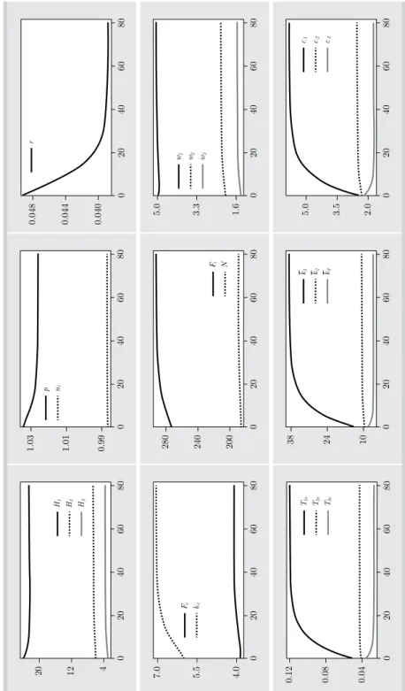
(16) 272. LATIN AMERICAN JOURNAL OF ECONOMICS | Vol. 50 No. 2 (Nov, 2013), 257–287. are specified around 0.05. The RC’s propensity to save is 0.8 and the PC’s propensity to save is 0.7 The value of the MC’s propensity is between the other groups. The RC’s propensity to obtain education is highest among the three classes; the PC has the lowest propensity to obtain education. Under (17) we find that the system has a unique equilibrium. The equilibrium values are listed in (18). The national industrial output is 292.25 and the interest rate is about 3.9 percent. The human capital levels of the RC, MC and PC are respectively 22.62, 6.63 and 3.64. The wage rates of the three groups are respectively 22.62, 6.63 and 3.64. The RC has the highest human capital as well as the highest wage rate. The RC also spends much more time in education than the other two groups. According to Dur and Glazer (2008), rich people tend to attend college at a higher rate than poor people, as rich people obtain more benefits from the consumption content of education. The PC spends the longest amount of time working. The RC’s consumption level and wealth are also highest. r = 0.039, p = 1.026, k = 5.67, N = 189.09, K = 1071.22, Fi = 292.25, Fe = 4.09,Ni = 186.61, Ne = 2.48, Ki = 1053.74, K e = 17.48, k i = 5.65, k e = 7.07, f i = 1.56, f e = 1.65, H1 = 22.62, H2 = 6.63, H3 = 3.64, w1 = 5.07, w2 = 2.27, – – – w3 = 1.57, k 1 = 38.96, k 2 = 10.57, k 3 = 6.07, T1e = 0.12,. (18). T2e = 0.04, T3e = 0.03, c1 = 5.84, c2 = 2.54, c3 = 1.74. It is straightforward to calculate the six eigenvalues as follows: –0.20, –0.18, –0.13, –0.09, –0.06, –0.03. As all the eigenvalues are negative, we see that the equilibrium is locally stable. We start with dif ferent initial states close to the equilibrium point and find that the system approaches the equilibrium point. In Figure 1, we plot the motion of the system with the following initial conditions: – – – k1(0) = 11, k2(0) = 4.5, k3(0) = 2, H1(0) = 3.5, H2(0) = 1.9, H3(0) = 0.5. The system approaches its equilibrium point in the long term.. (19).

(17) 0.04. 0.08. 0.12. 4.0. 5.5. 7.0. 4. 12. 20. 0. 0. 0. 20. 20. 20. ke. Fe. 40. 40. 40. 60. 60. 60. T3e. T2e. T1e. H3. H2. H1. 80. 80. 80. Figure 1. Motion of some variables. 10. 24. 38. 200. 240. 280. 0.99. 1.01. 1.03. 0. 0. 0. 20. 20. 20. ni. p. 40. 40. 40. 60. 60. 60. k3. k2. k1. N. Fi. 80. 80. 80. 2.0. 3.5. 5.0. 1.6. 3.3. 5.0. 0.040. 0.044. 0.048. 0. 0. 0. 20. 20. w3. w2. w1. 20. r. 40. 40. 40. 60. 60. 60. c3. c2. c1. 80. 80. 80. Wei-Bin Zhang | THE UZAWA-LUCAS MODEL WITH HETEROGENEOUS HOUSEHOLDS. 273.

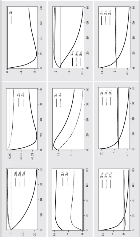
(18) 274. 4.. LATIN AMERICAN JOURNAL OF ECONOMICS | Vol. 50 No. 2 (Nov, 2013), 257–287. Comparative dynamic analysis. In simulating the motion of the dynamic system, it is important to ask questions such as how a change in one group’s propensity to save or to obtain education af fects the economy and each group’s wealth and consumption. First, we examine the case that all the parameters, except the RC’s propensity to obtain education, η10, are the same as in (17). We increase the propensity in the following way: η 10 : 0.015 ⇒ 0.018. The simulation results are plotted in – Figure 2. In the plots, a variable Δ x j(t ) stands for the change rate of the variable, x j(t), as a percentage, due to changes in the parameter value. From Figure 2 we see that as the RC increases the propensity to obtain education, the RC’s level of human capital is increased. To examine the process of the change in the human capital, we have to observe how all the variables in the system react to the parameter shift. Initially, as the rich class increases its preference for formal education, rich people would spend more time on schooling (with the other conditions remaining the same). Hence, the human capital of the rich class will be increased. The rise in human capital increases the total labor force, but the fall in work time reduces the labor force. As shown in Figure 2, the total labor force is reduced. Hence, the total output of the industrial sector falls. As the demand for education is increased, the education fee is increased and output of the education sector is increased. The labor share of the education sector is increased. Although the RC increases its education time, the education time of the other two classes is slightly af fected. The other two classes’ human capital levels are increased, but the PC’s human capital is much less af fected. The wage rate of the RC increases, but the wage rates of the other two classes fall. As the education hours of the MC and PC are slightly af fected, we can conclude that the returns from schooling in terms of wage rate are reduced for the two classes. As the RC puts more resources into schooling, wealth and consumption are reduced. It should be noted that in a model with education and inequality developed by Nakajima and Nakamura (2009), they find that the educational expenditure of rich households could prevent poor households from escaping poverty. Their model attempts to explain the possible ef fects of high prices of education on growth and inequality in countries such as Japan, Korea, and the U.S. The basic insight from the model is that as rich households demand higher.

(19) 0. 8. 16. 0.0. 2.5. 5.0. 0.0. 0.4. 0.8. 0. 0. 0. 20. 20. 20. ΔH3. ΔH2. ΔH1. 40. 40. 40. 60. 60. 60. 80. 80. ΔT2e. ΔT1e. Δke. ΔFe. 80. -2.4 0. 20. 40. 60. 60. 60. Δk 1. ΔN. ΔFi. Δk 3. Δk 2. 80. 80. 80. -0.10. 0.05. 0.20. -2.4. -1.2. 40. 40. -1.2. 20. 20. 0.0. 0.3. 0.0. 0. 0. Δni. Δp. 0.6. 0.0. -0.60. -0.45. -0.30. -0.06. -0.02. 0.02. Figure 2. A rise in the rich class’s propensity to obtain education. 0. 0. 0. 20. Δc3. Δc2. Δc1. 20. Δw 3. Δw 2. Δw 1. 20. 40. 40. 40. 60. 60. 60. Δr. 80. 80. 80. Wei-Bin Zhang | THE UZAWA-LUCAS MODEL WITH HETEROGENEOUS HOUSEHOLDS. 275.

(20) 276. LATIN AMERICAN JOURNAL OF ECONOMICS | Vol. 50 No. 2 (Nov, 2013), 257–287. education, the price is expected to rise, excluding the poor from higher education. This also leads to greater inequality between the rich and poor in the long term. Our model predicts similar ef fects in a country with heterogeneous households. We now increase the RC’s propensity to save in the following way: λ10: 0.8 ⇒ 0.85. The simulation results are plotted in Figure 3. As the RC increases the propensity to save, its wealth per capita rises. The society’s total capital is increased. As more capital is accumulated in the society, the interest rate falls. The increased capital results in higher wage rates. As wage rates rise, the opportunity costs of education are increased, which initially results in the reduction of education time for the three classes. As the RC accumulates more wealth and the RC’s wage rate is increased, we see that the RC increases its education time in the long term. As the RC reduces education time and puts away more money for future consumption, its level of human capital falls initially. But in the long term the RC’s human capital is increased as the RC devotes more time to education, becomes more ef fective through learning by consuming (due to a higher consumption) and learning by producing (due to increased output level of the industrial sector). The other two classes’ consumption levels are increased but only slightly. The RC’s wealth is increased significantly, but the other two classes’ wealth is only slightly af fected. The total labor input is slightly af fected. Because the RC cares more about wealth accumulation, we see that the share of labor force in the education sector is reduced and that of the industrial sector is increased. It is interesting to note that the human capital levels of the MC and the PC are increased more than the RC and the education fee is also reduced; the MC and PC don’t experience increases in wealth and consumption. We see that a rise in the RC’s propensity to save tends to enlarge the gaps with the other two classes in terms of wealth and consumption levels, but tends to reduce gaps for human capital among the classes. It should be noted that in this study, we fix propensities. In reality, as extremely rich people have “too much” money to spend, the propensity to save tends to increase in the long term. It is also worth noting that the propensity to save in our model is dif ferent from that defined in neoclassical growth theory. In our model, the propensity to save is equal to the share of disposable income saved for the future, while in the Solow model the propensity to save is equal to the share of current income saved.

(21) -4. -2. 0. -0.4. 1.3. 3.0. 0.00. 0.12. 0.24. 0. 0. 0. 20. 20. 20. ΔH3. ΔH2. ΔH1. 40. 40. 40. 60. 60. 60. ΔT3e. ΔT2e. 80. 80. ΔT1e. Δke. ΔFe. 80. 0. 4. 8. 0.2. 0.4. 1.0. -0.14. -0.07. 0.00. 0. 0. 0. 20. 20. 20. 40. 40. 40. Figure 3. A rise in the rich class’s propensity to save. 60. 60. 60. Δk 3. Δk 2. Δk 1. 80. 80. 80. ΔN. ΔFi. Δni. Δp. -4.0. -1.5. 1.0. 0.0. 0.5. 1.0. -4. -2. 0. 0. 0. 0. 20. 20. 20. 40. 40. 40. 60. 60. 60. Δc3. Δc2. Δc1. 80. 80. 80. Δw 3. Δw 2. Δw 1. Δr. Wei-Bin Zhang | THE UZAWA-LUCAS MODEL WITH HETEROGENEOUS HOUSEHOLDS. 277.

(22) 278. LATIN AMERICAN JOURNAL OF ECONOMICS | Vol. 50 No. 2 (Nov, 2013), 257–287. for the future. Hence, in the Solow model the extent to which people accumulate wealth has a much weaker impact on saving behavior than in our model when the wealth per capita is extremely high. It can be seen that our model predicts enlarged income gaps between the rich and the poor over time, even though the human capital levels may not vary much between the two groups. It has been observed that the ef fect of population growth varies with the level of economic development and can be positive for some developed economies. Theoretical models of human capital predict situation-dependent interactions between population and economic growth.8 We now increase the RC’s population in the following way: – N1: 10 ⇒ 15. The simulation results are plotted in Figure 4. As the RC population increases, its human capital and wage rate falls over time. The schooling time, consumption level and wealth per capita of the RC rise initially and fall in the long term. The price of education falls, which benefits the MC and PC. As the output of the industrial sector is increased as a consequence of the population increase, the MC and PC learn more ef fectively through learning by producing. The human capital levels of both the MC and the PC are increased. In the long term, the per-capita consumption and wealth levels of the MC and the PC are increased. We see that the MC and PC benefit in the long term. We thus conclude that an increase in the RC’s population reduces gaps in income, wealth and consumption between the rich and the poor in the long term. Another important question is what will happen to dif ferent people and the national economy if the total productivity of the education sector is increased. We increase the total productivity in the following way: Ae: 0.8 ⇒ 0.9. The simulation results are plotted in Figure 5. The rise in productivity increases the human capital of all groups and reduces the price of education. As all the classes’ human capital levels are increased and the dif ferences in these increases are not large, the distribution of the total labor force is slightly af fected. The two sectors increase their output levels in the long term. The education time, wage rates, wealth and consumption levels of all the groups are increased in the long term. We thus conclude that an improvement in the ef ficiency of the educational system will benefit dif ferent people in the long term.. 8. See Ehlich and Lui (1997), Galor and Weil (1999), and Boucekkine et al. (2002)..

(23) 0. 7. 14. 0. 7. 14. -20. -10. 0. 0. 0. 0. 20. 20. 20. 40. 40. 40. 60. 60. 60. ΔT3e. ΔT2e. ΔT1e. Δke. 80. 80. 80. ΔFe. ΔH3. ΔH2. ΔH1. -10. 5. 20. 10. 12. -0.24. -0.12. 0.00. 0. 0. 0. Figure 4. A rise in the rich class’s population. 20. 20. 20. 40. 40. 40. 60. 60. 60. Δk 3. Δk 2. 80. 80. 80. Δk 1. ΔN. ΔFi. Δni. Δp. -10. 2. 14. -10. -4. 2. -8. -4. 0. 0. 0. 0. 20. 20. Δw 3. Δw 2. Δw 1. 20. 40. 40. 40. 60. 60. 60. Δc3. Δc2. Δc1. Δr. 80. 80. 80. Wei-Bin Zhang | THE UZAWA-LUCAS MODEL WITH HETEROGENEOUS HOUSEHOLDS. 279.

(24) 1. 3. 5. 0. 0. 0. 20. ΔT3e. ΔT2e. ΔT1e. 20. 40. 40. 60. 60. 80. 80. Δke. ΔFe. -1.2. -0.5. 0.2. -0.15. 0. 0. 0. 20. 20. 20. 40. 40. 40. 60. 60. 60. 80. Δk 3. Δk 2. Δk 1. 80. ΔN. ΔFi. 80. 0.34. -0.8. -0.3. 0.2. 0.0. 0.2. 80. 0.00. 60. 0.17. 0.00. 2. 40. Δni. Δp. 0.4. 20. -10. -5. 0. 0.15. 0. ΔH3. ΔH2. ΔH1. 4. 0.0. 0.3. 0.6. Figure 5. A rise in the education sector’s total productivity. 0. 0. 0. 20. 20. Δw 3. Δw 2. Δw 1. 20. 40. 40. 40. 60. 60. 60. 80. 80. 80. Δc3. Δc2. Δc1. Δr. 280 LATIN AMERICAN JOURNAL OF ECONOMICS | Vol. 50 No. 2 (Nov, 2013), 257–287.

(25) Wei-Bin Zhang | THE UZAWA-LUCAS MODEL WITH HETEROGENEOUS HOUSEHOLDS. 5.. 281. Concluding remarks. This paper proposes a growth model of heterogeneous households with wealth accumulation and human capital accumulation. The economic system consists of one production sector and one education sector. We consider three ways of improving human capital: learning by producing, learning by education, and learning by consuming. The model describes a dynamic interdependence among wealth accumulation, human capital accumulation, and division of labor under perfect competition. We simulated the model of three groups to demonstrate the existence of equilibrium points and motion in the dynamic system. We also examined the ef fects of changes in some parameters on the motion of the system. The model could be extended in several directions. For instance, as mentioned by Bertocchi and Spagat (2004), the specific structure of the educational system is largely unexplored. Education may be privately or publicly provided. An education system may also be founded on a hierarchical dif ferentiation between vocational and general education. As demonstrated in Bertocchi and Spagat, the educational structure varies over time. We could introduce some kind of government intervention in education into the model. In this study, we don’t consider public provision or subsidy of education. In the literature on education and economic growth, many models with heterogeneous households are proposed to address issues related to taxation, education policy, distribution of income and wealth, and economic growth. For instance, Bénabou (2002) studies the ef fects of progressive income taxes and education finance in a dynamic heterogeneous-agent model. As shown in Glomm and Kaganovich (2008), public provision may have a significant impact on growth and inequality across households. They examine the relationship between growth and inequality with public education in the context of an overlapping generations economy with heterogeneous agents. The government collects a tax on labor income to finance education. The model predicts that government spending on education reduces income inequality. Another study by Dur and Glazer (2008) shows that rich people tend to attend college at a higher rate than poor people, as rich people obtain more benefits from the consumption content of education. They conclude that to make sure that colleges attract the most competent students and not simply the richest, colleges should charge rich students higher tuition fees..

(26) 282. LATIN AMERICAN JOURNAL OF ECONOMICS | Vol. 50 No. 2 (Nov, 2013), 257–287. Appendix Proof of lemma 1 From (4) and (6), we obtain: Ke. =α. Ne. Ki Ni. , i.e., ke = α ki ,. (A1). where α ≡ αe βi / αi βe (≠ 1 assumed). From (A1), (4) and (6), we obtain: β. p=. α e αi Ai αe Ae. (A2). kiβ ,. where β ≡ βe βi – βi . From (A1) and (1), we solve the labor distribution as functions of k i and k : ni =. α ki − k. ( α − 1 )ki. , ne =. k − ki. ( α − 1 )ki. .. (A3). From (p + wj )Tje = ηjy–j in (11) and the definition of y–j we have:. Tje = φjp k j + φj 0 ,. (A4). where: φjp ( ki , H j ) ≡. (1 + r ) ηj p + wj. , φj 0 ( ki , H j ) ≡. η j T0 w j p + wj. .. From (A4) and (14): J. φ ∑ ( φjp k j + φj 0 ) N j = N ( k − ki ), j =1. α. where we also use Fe = Aeke e neN, (A3), ke = αki , and: φ ( ki ) ≡. ( α − 1 )kiβ. e. αe. α Ae. .. (A5).

(27) , { k j }) ≡. 283. Wei-Bin Zhang | THE UZAWA-LUCAS MODEL WITH HETEROGENEOUS HOUSEHOLDS. From Tj + Tje = T0 and (A4), we have: Tj = T0 − φjp k j − φj 0 .. (A6). From (A6), we have: N =. J. ∑ (T0 − φjp k j j =1. m. − φj 0 ) H j j N j .. (A7). From (2) and K = kN, we have:   J m  K = k  ∑ (T0 − φjp k j − φj 0 ) H j j N j  .  j =1 . (A8). From (A8) and (15), we have:   J m  k N = k  ∑ (T0 − φjp k j − φj 0 ) H j j N j  =  j =1 . J. ∑ kj N j .. (A9). j =1. Insert (A9) and (A7) in (A5): k1 = Λk ( ki , ( H j ), { k j } ) ≡. m. Λ0 − φ φ10 − (T0 − φ10 ) ki H 1 1 m. φ φ1p − 1 − φ1p ki H 1 1. ,. (A10). where: Λ0 ( ki , ( H j ), { k j } ) ≡. J. 1 m ∑  k − (T0 − φjp k j − φj 0 )ki H j j − φ ( φjp k j + φj 0 )  N j , N1 j =2  j. J. 1  k − T − φ k − φ k H mj − φ φ k + φ  N , ( 0 jp j ( jp j ∑  j0 ) i j j 0 ) j  N1 j =2  j. –. –. –. where (Hj) ≡ (H1,…,HJ) and {k j } ≡ (k 2,…,k J). It is straightforward to confirm that all the variables can be expressed as functions of ki , (Hj) – and {k j } by the following procedure: ke by (A1) → r and wj by (4) → p – by (A2) → k 1 by (A10) → k by (A9) → K by (A8) → Tj by (A6) → Tje by (A4) → N by (A7) → ni and ne by (A3) → Ni = ni N and Ne = neN → Ki = ki Ni and Ke = keNe → Fi by (4) → Fe by (5) → y–j by (9) → cj and sj by (11). From this procedure and (11), we have:.

(28) }) ≡. 284. LATIN AMERICAN JOURNAL OF ECONOMICS | Vol. 50 No. 2 (Nov, 2013), 257–287. a je. H j = Λ j ( k1i , ( H j ), { k j } ) ≡. a υje Fe je. (. m Hj j π. Tje N j. H j je N j. bje. ). a ji. +. υji Fi π. H j ji N j. υje Fe. (H. mj j. Tje N j. π. H j je N j. bje. ). a ji. +. υji Fi π. H j ji N j. a. +. υjh C j jh H jπh N j (A11). a. +. υjh C j jh. − δjh H j .. H jπh N j. Here, we don’t provide explicit expressions of the functions as they are – tedious. Substituting y–j = (1 + r)k j + T0wj in sj = λj y–j yields: s j = ( 1 + r ) λj k j + λj T0 w j .. (A12). Substituting (A12) in (12), we have: k1 = λ1 T0 w1 − R ( ki , H 1 ) k1 ,. (A13). kj = Λ j ( ki , ( H j ), { k j } ) ≡ λj T0 w j − ( 1 − λj − λj r ) k j , j = 2, ..., J ,. (A14). ki , ( H j ), { k j }) ≡ λj T0 w j − ( 1 − λj − λj r ) k j , j = 2, ..., J ,. in which R(k i, H1) ≡ 1 – λ1– λ1r. Taking derivatives of equation (A10) with respect to t yields: ∂ Λk k1 = k + ∂ ki i. J. ∂Λ. ∑ Λ j ∂ Hk j =1. j. J. +. ∑ Λj j =2. ∂ Λk ∂ kj. (A15). ,. where we use (A11) and (A14). Equaling the right-hand sides of equations (A13) and (A15), we get:  λ1 T0 w1 − R Λk   ki = Λ1 ( ki , ( H j ), {k j } ) ≡  J ∂ Λk  −  − ∑ Λj  j =1 ∂ H j .     ∂ Λk J ∂ Λk   ∑ Λ j ∂ k   ∂ ki j =2 j . −1  . (A16)  . In summary, we have proved Lemma 1. ■. − δjh H j ..

(29) Wei-Bin Zhang | THE UZAWA-LUCAS MODEL WITH HETEROGENEOUS HOUSEHOLDS. 285. References Aakvik, A., K.G. Salvanes, and K. Vaage (2010), “Measuring heterogeneity in the returns to education using an education reform,” European Economic Review 54: 453–500. Abel, A.B. and B.S. Bernanke (1998), Macroeconomics, 3rd edition. New York: Addison-Wesley. Aghion, P. and P. Howitt (1998), Endogenous growth theory. Cambridge: The MIT Press. Arrow, K.J. (1962), “The economic implications of learning by doing.” Review of Economic Studies 29: 155–73. Attanasio, O.P. and G. Weber (2010), “Consumption and saving: Models of intertemporal allocation and their implications for public policy,” NBER Working Paper 15756. Azariadis, C. (1993), Intertemporal macroeconomics. Oxford: Blackwell. Banerjee, A.V. (2004), “Educational policy and the economics of the family,” Journal of Development Economics 74: 3–32. Barro, R.J. (2001), “Human capital and growth,” American Economic Review, Papers and Proceedings 91: 12–17. Barro, R.J. and X. Sala-i-Martin (1995), Economic growth. New York: McGrawHill, Inc. Becker, G. (1981), A treatise on the family. Cambridge: Harvard University Press. Behrman, J., R. Pollak, and P. Taubman (1982), “Parental preferences and provision for progeny,” Journal of Political Economy 90: 52–73. Bénabou, R. (2002), “Tax and education policy in a heterogeneous-agent economy: What levels of redistribution maximize growth and ef ficiency?” Econometrica 70: 481–517. Bertocchi, G. and M. Spagat (2004), “The evolution of modern educational systems: Technical vs. general education, distributional conflict, and Growth,” Journal of Development Economics 73: 558–82. Boucekkine, R., D. de la Croix, and O. Licandro (2002), «Vintage human capital: Demographic trends and endogenous growth,” Journal of Economic Growth 104: 340–75. Burmeister, E. and A.R. Dobell (1970), Mathematical theories of economic growth. London: Collier Macmillan Publishers. Cardak, B.A. (2004), “Education choice, endogenous growth and income distribution,” Economica 71: 57–81. Castelló-Climent, A. and A. Hidalgo-Cabrillana (2012), “The role of education quality and quantity in the process of economic development,” Economics of Education Review (forthcoming). Chen, M.K. and J.A. Chevalier (2008), “The taste for leisure, career choice, and the returns to education,” Economics Letters 99: 353–56..

(30) 286. LATIN AMERICAN JOURNAL OF ECONOMICS | Vol. 50 No. 2 (Nov, 2013), 257–287. Could, E.D., O. Moav, and B.A. Weinberg (2001), “Precautionary demand for education, inequality, and technological progress,” Journal of Economic Growth 6: 285–315. Cox, D. (1987), “Motives for private income transfers,” Journal of Political Economy 95: 508–46. Dur, R. and A. Glazer (2008), “Subsidizing enjoyable education,” Labour Economics 15: 1023–39. Easterlin, R. (1981), “Why isn’t the whole world developed?” Journal of Economic History 41: 1–19. Ehrlich, I. and F. Lui (1997), “The problem of population and growth: A review of the literature from Malthus to contemporary models of endogenous population and endogenous growth,” Journal of Economic Dynamics and Control 21: 205–4. Erosa, A., T. Koreshkova, and D. Restuccia (2010), "How important is human capital? A quantitative theory assessment of world income inequality," The Review of Economic Studies 77: 1421–49. Fender, J. P. and Wang (2003), "Educational policy in a credit constrained economy with skill heterogeneity," International Economic Review 44: 939-64. Fernandez, R. and R. Rogerson (1998), “Public education and income distribution: A dynamic quantitative evaluation of education finance reform,” American Economic Review 88: 813–33. Fleisher, B., Y.F. Hu, H.Z. Li, and S.H. Kim (2011), “Economic transition, higher education and worker productivity in China,” Journal of Development Economics 94: 86–94. Frederick, S., G. Loewenstein, and T. O’Donoghue (2002), “Time discontinuing and time preference: A critical review,” Journal of Economic Literature 40: 351–401. Galor, O. and O. Moav (2004), “From physical to human capital accumulation: Inequality in the process of development,” Review of Economic Studies 71: 1001–26. Galor, O. and D. Weil (1999), “From Malthusian stagnation to modern growth,” American Economic Review 89: 150–54. Galor, O. and J. Zeira (1993), “Income distribution and macroeconomics,” Review of Economic Studies 60: 35–52. Glomm, G. and M. Kaganovich (2008), “Social security, public education and the growth-inequality relationship,” European Economic Review 52: 1009–34. Grossman, G.M. and E. Helpman (1991), Innovation and Growth in the Global Economy. Cambridge: The MIT Press. Hanushek, E. and D. Kimko (2000), “Schooling, labor-force quality and the growth of nations,” American Economic Review 90: 1194–204. Heckman, J.J. (1976), “A life-cycle model of earnings, learning, and consumption,” Journal of Political Economy 84: S11–44..

(31) Wei-Bin Zhang | THE UZAWA-LUCAS MODEL WITH HETEROGENEOUS HOUSEHOLDS. 287. Krueger, A.B. and M. Lindahl (2001), “Education for growth: Why and for whom,” Journal of Economic Literature 39: 1101–36. Laitner, J. (2000), “Earnings within education groups and overall productivity growth,” Journal of Political Economy 108: 807–32. Lazear, E. (1977), “Education: Consumption or production,” Journal of Political Economy 85: 569–97. Lucas, R.E. (1988), “On the mechanics of economic development,” Journal of Monetary Economics 22: 3–42. Malchow-Møller, N., S. Nielsen, and J.R. Skaksen (2011), "Taxes, tuition fees, and education for pleasure," Journal of Public Economic Theory 13: 189–215. Maoz, Y.D. and O. Moav (1999), “Intergenerational mobility and the process of development,” Economic Journal 109: 677–97. Mincer, J. (1974), Schooling, experience and earnings. New York: Columbia University Press. Nakajima, T. and H. Nakamura (2009), “The price of education and inequality,” Economics Letters 105: 183–85. Romer, P.M. (1986), “Increasing returns and long-run growth,” Journal of Political Economy 94: 1002–37. Solow, R. (2000), Growth theory – An exposition. New York: Oxford University Press. Tilak, J.B.C. (1989), Education and Its Relation to Economic Growth, Poverty and Income Distribution: Past Evidence and Future Analysis. Washington, D.C.: World Bank. Tselios, V. (2008), "Income and educational inequalities in the regions of the European Union: Geographical spillovers under welfare state restrictions," Papers in Regional Science 87: 403–30. Uzawa, H. (1965), “Optimal technical change in an aggregative model of economic growth,” International Economic Review 6: 18–31. Zhang, W.B. (2005), Economic Growth Theory. London: Ashgate. Zhang, W.B. (2007), “Economic growth with learning by producing, learning by education, and learning by consuming,” Interdisciplinary Description of Complex Systems 5: 21–38. Zhang, W.B. (2009), “A discrete one-sector growth model with endogenous labor supply and heterogeneous groups,” Discrete Dynamics in Nature and Society 2009. Zhu, R. (2011), “Individual heterogeneity in returns to education in urban China during 1995-2002,” Economics Letters 113: 84–7..

(32)

(33)