arXiv:1502.01118v1 [stat.ME] 4 Feb 2015
(will be inserted by the editor)
Robust estimation of mixtures of regressions with random
covariates, via trimming and constraints
L.A. Garc´ıa-Escudero · A. Gordaliza · F. Greselin · S. Ingrassia · A. Mayo-Iscar
Received: date / Accepted: date
Abstract A robust estimator for a wide family of mixtures of linear regression is
pre-sented. Robustness is based on the joint adoption of the Cluster Weighted Model and of an estimator based on trimming and restrictions. The selected model provides the conditional distribution of the response for each group, as in mixtures of regression, and further supplies local distributions for the explanatory variables. A novel version of the restrictions has been devised, under this model, for separately controlling the two sources of variability identified in it. This proposal avoids singularities in the log-likelihood, caused by approximate local collinearity in the explanatory variables or local exact fits in regressions, and reduces the occurrence of spurious local maxi-mizers. In a natural way, due to the interaction between the model and the estimator, the procedure is able to resist the harmful influence of bad leverage points along the estimation of the mixture of regressions, which is still an open issue in the literature. The given methodology defines a well-posed statistical problem, whose estimator ex-ists and is consistent to the corresponding solution of the population optimum, under widely general conditions. A feasible EM algorithm has also been provided to obtain the corresponding estimation. Many simulated examples and two real datasets have been chosen to show the ability of the procedure, on the one hand, to detect anoma-lous data, and, on the other hand, to identify the real cluster regressions without the influence of contamination.
Keywords Cluster Weighted Modeling·Mixture of Regressions·Robustness·
Trimming·Constrained estimation.
L.A. Garc´ıa-Escudero, A. Gordaliza, A. Mayo-Iscar
Department of Statistics and Operations Research and IMUVA, University of Valladolid, Valladolid, Spain E-mail: [email protected]; [email protected], [email protected]
F. Greselin
Department of Statistics and Quantitative Methods, Milano-Bicocca University, Milano, Italy E-mail: [email protected]
S. Ingrassia
1 Introduction
Mixture models provide a quite flexible approach to statistical modeling of a wide va-riety of random phenomena, whenever we can reasonably suppose that the observa-tions arise from unobserved groups in the population. Under this general framework, the present paper provides a new proposal in the family of finite mixtures of robust regressions (DeSarbo and Cron, 1988; de Veaux, 1989).
Assume we are provided with two quantitative random variablesX andY:X is a vector of explanatory variables,Y is a response or outcome variable, and the dependence betweenY andXmay vary among the different underlying groups. By adopting the cluster-weighted approach, we allow different scatter structures in each group, both in the marginal distribution ofXand in the conditional distribution of
Y|X=x, as it is required by many observed dataset. The Cluster Weighted Model (CWM), introduced in Gershenfeld (1997), decomposes the joint p.d.f. of(X, Y)in each component of the mixture as the product of the marginal and the conditional distributions.
Additionally, a restricted approach not only avoids singularities, it also discards non-interesting local maximizers of the objective function (Garc´ıa-Escudero et al., 2014b). We will discuss in detail how approximate local collinearity in the explanatory vari-ables, and approximate local exact fits in the regressions may cause, indeed, serious troubles in CWMs.
The above considerations give rise to the robust estimation of the trimmed Clus-ter Weighted Restricted Model (trimmed CWRM) presented hereafClus-ter. It includes an original application of the constraints, which takes into account the specific features of CWM and controls the relative variability between components for the sources of variability in the model corresponding to: i) the explanatory variables, and ii) the regression errors. The CWM, endowed with restrictions and trimming, becomes a very competitive robust estimator for mixtures of multiple regression, with optimal statistical properties.
We have organized the paper as follows. In Section 2 we recall the main ideas about the CWM. In Section 3 we present the trimmed CWRM, and introduce a feasi-ble algorithm for its practical implementation. Then, we state the central findings of the paper, i.e. the existence and the strong consistency of the new estimator. Section 4 provides a discussion on the effects of constraints and trimming, along with some illustrative examples. The application of the proposed methodology to two real data sets is shown in Section 5. Finally, Section 6 contains some concluding remarks and sketches future research. Proofs and technical lemmas needed for our main results are relegated in the Appendix.
2 Cluster Weighted Modeling
The Cluster Weighted Model (CWM) has been proposed in the context of media tech-nology, to build a digital violin with traditional inputs and realistic sounds (Gershenfeld, 1997; Gershenfeld et al., 1999); in Wedel (2000). CWMs are referred to as the fam-ily of saturated mixture regression models. In Ingrassia et al. (2012), CWMs have been reformulated in a statistical setting showing that they are a general and flexible family of mixture models. In fact, Ingrassia et al. (2012) show that Gaussian CWM includes, as special cases, finite mixtures of distributions and finite Mixtures of Re-gression models.
Let(X, Y)be a pair of random variables, namely a vector of covariatesXand a response variableY defined onΩwith values inX × Y ⊆Rd×Rand{(xi, yi)}ni=1 represents a i.i.d. random sample of sizen, drawn from(X, Y). Letp(x, y)denote the joint density of(X, Y), and suppose thatΩcan be partitioned intoGgroups, say
Ω1, . . . , ΩG. CWMs are mixture models having density of the form
p(x, y;θ) =
G
X
g=1
p(y|x;ξ
g)p(x;ψg)πg, (1)
wherep(y|x;ξ
g)is the conditional density ofY givenxinΩg(depending on some
parameterξg),p(x;ψ
g)is the marginal density ofXinΩg(depending on some
1). Furthermore, we assume that in each groupΩg, the conditional expectation of Y givenX=x, is a functionm(·)ofxdepending on some parametersβg, that is E(Y|x, Ωg) =m(x;βg).
In this work, we have focused on models of type (1) with Gaussian components. Thusp(x;ψ
g) =φd(x;µg,Σg), whereφd(·;µg,Σg)denotes the density of thed
-variate Gaussian distribution with mean vectorµgand covariance matrixΣg.
More-over, we have assumed that the conditional relationship betweenY andxin theg -th group can be written as Y = b′gx+b0g +εg whereεg ∼ N(0, σg2). Hence,
X|Ωg ∼Nd(µg,Σg)andY|x, Ωg ∼N(b′gx+b0g, σg2), so that model (1) special-izes to:
p(x, y;θ) =
G
X
g=1
φ(y;b′
gx+b
0
g, σg)φd(x;µg,Σg)πg, (2)
which defines the linear Gaussian CWM. We notice here that definition (2) corre-sponds to a mixture of regressions, with weightsφd(x;µg,Σg)πg depending also
on the covariate distributions in each componentgforg = 1, . . . , G. Finally, in the framework of model-based clustering, each unit is assigned to one group, based on the maximum a posteriori probability. The consideration of (2) yields to the use of (log-)likelihood target function to be maximized as
n
X
i=1 log
" G X
g=1
φ(yi;b′gxi+b0g, σg2)φd(xi;µg,Σg)πg
#
. (3)
For sake of simplicity, we will later use the notation
Dg(x, y;θ) =φ(y;b′gx+b0g, σ2g)φd(x;µg,Σg)πg
andD(x, y;θ) = PG
g=1Dg(x, y;θ), where the set of all parameters of the model
is denoted byθ, and, such that (3) is simply rewritten as Pni=1log[D(xi, yi;θ)]. Additionally, the linear Gaussian CWM will be many times simply referred to as CWM.
2.1 Two problems about CWM
−5 0 5 10 15 20
−5
0
5
10
15
(a)
0 5 10 15
2
4
6
8
10
(b)
−5 0 5 10 15 20
0
5
10
15
(c)
0 5 10 15
2
4
6
8
10
(d)
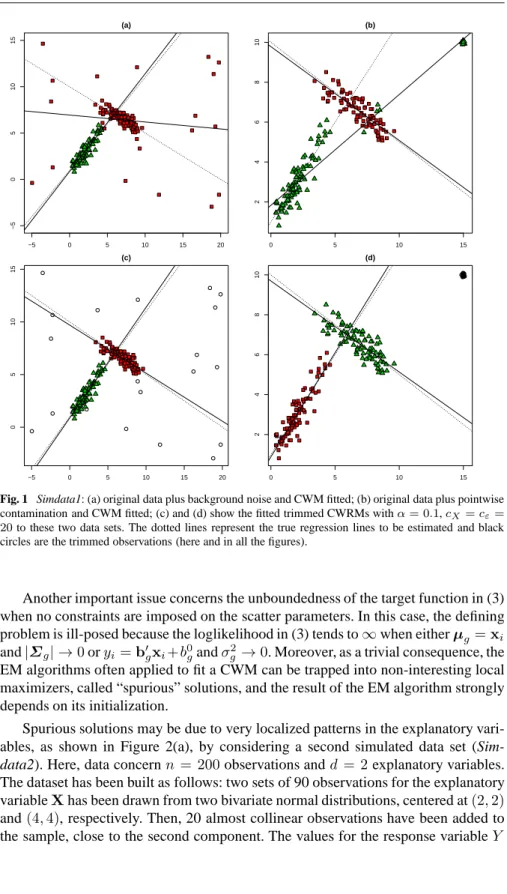
Fig. 1 Simdata1: (a) original data plus background noise and CWM fitted; (b) original data plus pointwise
contamination and CWM fitted; (c) and (d) show the fitted trimmed CWRMs withα= 0.1,cX=cε=
20to these two data sets. The dotted lines represent the true regression lines to be estimated and black circles are the trimmed observations (here and in all the figures).
Another important issue concerns the unboundedness of the target function in (3) when no constraints are imposed on the scatter parameters. In this case, the defining problem is ill-posed because the loglikelihood in (3) tends to∞when eitherµg=xi and|Σg| →0oryi=b′gxi+b0gandσg2→0. Moreover, as a trivial consequence, the
EM algorithms often applied to fit a CWM can be trapped into non-interesting local maximizers, called “spurious” solutions, and the result of the EM algorithm strongly depends on its initialization.
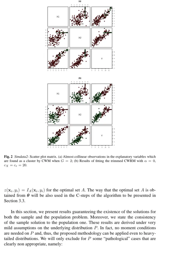
have been generated by using the same linear function (for both components) with equally distributed error terms. We can see in Figure 2(a) that the standard fit of the CWM yields to the determination of a first spurious component with the 20 almost collinear observations and a second component joining together the two groups, with 90%of the observations.
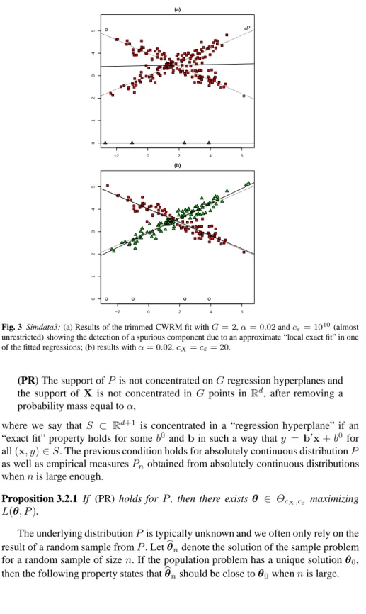
Sometimes spurious solutions may be also due to localized patterns of obser-vations, where an approximate “exact fit” for a small number of observations can be obtained. Figure 3 shows a third simulated data set (Simdata3) withn= 200 observa-tions, where 196 of them have been generated from a CWM withG= 2components (98 observations from each component). A very small fraction of almost collinear units (only 4 observations) on the(X, Y)variables have been added, with a roughly equal value (around0) for the response variable. These values, for instance, could be due to a bad performance of the tool used to measure the response variable. It may be seen that a fitted component including only these almost collinear observations could arise, along the EM estimation, because a small value of one of theσ2
g parameters
yields to higher values of the log-likelihood. Then, the two main linear structures accounting for98%of the data points would be artificially joined together.
To overcome the previous issues, in the next section we propose a robust method-ology by incorporating trimming and constraints to the CWM.
3 Trimmed Cluster Weighted Restricted Modeling
3.1 Problem statement
For a given sample ofnobservations, the trimmed CWRM methodology is based on the maximization of the following log-likelihood function
n
X
i=1
z(xi, yi) log
"G X
g=1
φ(yi;b′gxi+b0g, σg2)φd(xi;µg,Σg)πg
#
, (4)
wherez(·,·)is a 0-1 trimming indicator function that tell us whether observation (xi, yi)is trimmed off (z(xi, yi)=0), or not (z(xi, yi)=1). A fixed fractionαof ob-servations can be unassigned by setting Pni=1z(xi, yi) = [n(1−α)]. Hence the parameterαdenotes the trimming level. Analogous approaches based on trimmed mixture likelihoods can be found in Neykov et al. (2007), Gallegos and Ritter (2009) and Garc´ıa-Escudero et al. (2014b).
Moreover, we introduce two further constraints on the maximization in (4). The first one concerns the set of eigenvalues{λl(Σg)}l=1,...,dof the scatter matricesΣg
by imposing
λl1(Σg1)≤cXλl2(Σg2) for every1≤l16=l2≤dand1≤g16=g2≤G.
(5) The second constraint refers to the variancesσ2
gof the regression error terms, by
requiring
σ2g1≤cεσ
2
The constantscXandcε, in (5) and (6) respectively, are finite (not necessarily equal)
real numbers, such that cX ≥ 1, cε ≥ 1. They automatically guarantee that we
are avoiding the|Σg| → 0 andσ2
g → 0cases. These constraints are an extension
to CWMs of those introduced in Ingrassia and Rocci (2007), Garc´ıa-Escudero et al. (2008) and Greselin and Ingrassia (2010) and go back to Hathaway (1985). The main difference is the asymmetric and different treatment given by the constraints, when modeling the marginal distributionXor when modeling the regression error terms, providing high flexibility to the model.
Let us consider now the effects of trimming in the two data sets derived from Simdata1. In Figure 1(c) and (d) we can see that settingα= 0.1allows to restore the true structure of the data, by discarding the outlying observations, both in the case of background noise and pointwise contamination. Hence, trimming modifies the ML estimation in such a way that it is no more influenced by potential outliers and drives it far from the previous bad results.
Commenting the use of constraints, we can see how a moderate choice ofcXfor
Simdata2 in Figure 2(b) allows to correctly detect theG = 2main groups and to avoid the disturbing effect of the spurious patterns in the explanatory variables.
Additionally, we can see that a moderate choice of cεfor Simdata3 would also
allow to correctly detect theG = 2main groups. Moreover, we can see in Figure 3(a) how only consideringα= 0.02trimming level (trying to discard the 4 outlying observations in Simdata3) does not solve the problem at all without the consideration of a moderate value ofcε.
A detailed discussion about the role played byα,cXandcεis given in Section 4.
3.2 Theoretical results
The problem stated in Section 3.1 admits a population counterpart. LetP =P(X,Y) be the probability measure inRd+1 induced by the joint distribution of the random variablesXandY and letEP(·)denote the expectation with respect toP. LetΘcX,cε
denote hereafter the set of all possibleθ which do satisfy constraints (5) and (6) for given constantscXandcε. With this notation, the population problem is defined
through the double maximization ofEP
logD(X, Y;θ)IA(X, Y)
over all possible
θ∈ΘcX,cε, and over all possible subsetsA⊂R
d+1, withP[A]≥1−α. As usual,
IA(·)denotes the indicator function of setA. We will see that the optimal setAcan
be determined directly fromθ. In more detail, fixedθ, and denoting by
R(θ, P) = sup
u
u:P[(X, Y) :D(X, Y;θ)≥u]≥1−α ,
thenAis given byA(θ) =A(θ, P) ={(x, y) :D(x, y;θ)≥R(θ, P)}.Therefore, we reduce the population problem to that of maximizing
L(θ, P) =EP
logD(X, Y;θ)I
A(θ)(X, Y)
, onθ∈ΘcX,cε (7)
X1
0 1 2 3 4 5 6
0
1
2
3
4
5
6
7
0
1
2
3
4
5
6
X2
0 1 2 3 4 5 6 7 2 4 6 8 10 12
2
4
6
8
10
12
Y (a)
X1
0 1 2 3 4 5 6
0
1
2
3
4
5
6
7
0
1
2
3
4
5
6
X2
0 1 2 3 4 5 6 7 2 4 6 8 10 12
2
4
6
8
10
12
Y (b)
Fig. 2 Simdata2: Scatter plot matrix. (a) Almost collinear observations in the explanatory variables which
are found as a cluster by CWM whenG= 2; (b) Results of fitting the trimmed CWRM withα= 0,
cX=cε= 20.
z(xi, yi) = IA(xi, yi)for the optimal setA. The way that the optimal setAis ob-tained fromθ will be also used in the C-steps of the algorithm to be presented in Section 3.3.
−2 0 2 4 6
0
1
2
3
4
5
(a)
−2 0 2 4 6
0
1
2
3
4
5
(b)
Fig. 3 Simdata3: (a) Results of the trimmed CWRM fit withG= 2,α= 0.02andcε= 1010(almost
unrestricted) showing the detection of a spurious component due to an approximate “local exact fit” in one of the fitted regressions; (b) results withα= 0.02,cX=cε= 20.
(PR) The support ofP is not concentrated onGregression hyperplanes and the support of Xis not concentrated in G points inRd, after removing a probability mass equal toα,
where we say that S ⊂ Rd+1 is concentrated in a “regression hyperplane” if an “exact fit” property holds for someb0 andbin such a way thaty = b′x+b0 for all(x, y)∈S. The previous condition holds for absolutely continuous distributionP
as well as empirical measuresPn obtained from absolutely continuous distributions
whennis large enough.
Proposition 3.2.1 If (PR) holds for P, then there existsθ ∈ ΘcX,cε maximizing
L(θ, P).
The underlying distributionPis typically unknown and we often only rely on the result of a random sample fromP. Letbθndenote the solution of the sample problem
Proposition 3.2.2 Assume thatPbe an absolutely continuous distribution with strictly positive density function satisfying (PR) and that θ0 is the unique maximizer of
L(θ, P)forθ ∈ ΘcX,cε. If{θbn}
∞
n=1 ⊂ΘcX,cεis a sequence of maximizers of (7)
whenP is replaced by the sequence of empirical measures{Pn}∞n=1, referred to a sequence of i.i.d. samples fromP, thenθbn →θ0almost surely.
Note that, apart from the (PR) condition, a uniqueness condition is also needed to get consistency. It is also important to note that the parameters obtained by solving the maximization (7) do not necessarily coincide with the parameters of the mixture components appearing in the definition of the (uncontaminated) CWM. However, we conjecture that these two different types of parameters are “close” each other when-ever the contamination is not very overlapped with the most interior regions of the mixture components and whenα,cXandcεare “properly” chosen. However,
estab-lishing results formalizing this idea is not an easy task (as happens even in simpler clustering approaches).
Although the proofs of these theoretical results, given in the Appendix, are re-lated to previous works in Garc´ıa-Escudero et al. (2008) and Garc´ıa-Escudero et al. (2014a), several specific technicalities must be sorted out for the present case. In fact, these technicalities are far from being straightforward and mainly have to do with how to deal with the effect of “local collinearities” in the regression coefficients.
3.3 Algorithm
The constrained maximization of the trimmed log-likelihood in (4) on its parame-ters is not an easy task. In this section, we present a feasible algorithm obtained by combining the EM algorithm for CWM with that (with trimming and constraints) introduced in Garc´ıa-Escudero et al. (2014b) (see, also, Fritz et al., 2013):
1. Initialization: The algorithm is initialized several times by selecting different ini-tial θ(0) = (π(0)1 , ..., π(0)G ,µ(0)1 , ...,µG(0),Σ(0)1 , ...,Σ(0)G , b0(0)1 , ..., b0(0)G ,b(0)
1 , ..., b(0)
G , σ
2(0) 1 , ..., σ
2(0)
G ). After drawingd+ 2distinct observations for each group,
we compute their sample means and sample covariance matrices as initial values forµ(0)g andΣ(0)g . Additionally,Gordinary least square regressions are carried
out to obtain initialb0(0)g andb(0)g regression parameters (G-inverse matrices are
used if needed). The mean square errors of the G regressions are used to de-termine the initialσ2(0)g values. IfΣ(0)g and/orσ
2(0)
g do not satisfy the required
constraints (5) and (6) then the procedure that will be described in Step 2.2 is applied to enforce them. Finally, weightsπ1(0), ..., πG(0) in the interval(0,1)and summing up to 1 are randomly chosen.
2.1. E- and C-steps: Letθ(l)be the parameters at iterationl, we computeDi = D(xi, yi;θ(l))fori= 1, ..., n. After sorting these values, the notationD(1) ≤
....≤D(n)is adopted. Let us consider the subset of indicesI⊂ {1,2, ..., n} defined asI = i : D(i) ≥ D([nα]) .To update the parameters, we will
take into account only the observations with indices inI, by settingτig(l) =
Dg(xi, yi;θ(l))/D(xi, yi;θ(l))fori ∈ Iandτig(l) = 0fori /∈ I. Note that τig(l), for the observations with indices inI, are the usual “posterior
probabili-ties” in the standard EM algorithm.
2.2. M-step: From theseτigvalues, we update the weight and mean parameters as
π(gl+1)= n
X
i=1
τig(l)/[n(1−α)] and µ(gl+1)= n
X
i=1
τig(l)xi
Xn
i=1
τig(l).
The other parameters (regression and scatter ones) are initially updated by
Tg= n
X
i=1
τig(l)(xi−µ(l+1)
g )(xi−µ(gl+1))′
Xn
i=1
τig(l),
b(l+1)
g = n X i=1
τig(l)xix′
i
Xn
i=1
τig(l)− n
X
i=1
τig(l)x′
i
Xn
i=1
τig(l)
!2
−1 × n X i=1
τig(l)yix′i
Xn
i=1
τig(l)− n
X
i=1
τig(l)yi
Xn
i=1
τig(l)· n
X
i=1
τig(l)x′
i
Xn
i=1
τig(l)
!
,
b0(gl+1)= n
X
i=1
τig(l)yi
Xn
i=1
τig(l)−(b(gl+1))′ n
X
i=1
τig(l)x′i
Xn
i=1
τig(l)
s2g=
n
X
i=1
τig(l)
yi−(b(gl+1))
′x
i−b0(gl+1)
2Xn
i=1
τig(l).
Along the iterations, due to the updates, it may happen that theTgmatrices
and thes2
gvalues do not satisfy the required constraints for the scatter
param-eters.
To perform a constrained maximization of the sample covariance matrices, the singular-value decomposition ofTg=Ug′EgUgis considered, withUgbeing
an orthogonal matrix andEg=diag(eg1, eg2, ..., egd)a diagonal matrix.
Af-ter defining the truncated eigenvalues as[egl]Xm= min cX·m,max(egl, m)
,
withmbeing some threshold value, then the scatter matrices are finally up-dated asΣ(gl+1)=U′
gEg∗Ug,withEg∗=diag
[eg1]XmX
opt,[eg2]
X mX
opt, ...,[egp]
X mX
opt
andmX
optminimizing the real valued function
m7→ G
X
g=1
π(l+1)
g d
X
l=1
log [egl]Xm
+ egl [egl]Xm
. (8)
Analogously, in case that thes2
j parameters do not satisfy the constraint (6),
we consider the truncated variances[s2
g]εm= min cε·m,max(s2g, m)
variances of the error terms are finally updated asσ2(gl+1) = [s2g]εmε
opt, with mε
optminimizing the real valued function
m7→ G
X
g=1
π(l+1)
g log [s2g]εm
+ s 2
g
[s2
g]εm
!
. (9)
Proposition 3.2 in Fritz et al. (2013) shows thatmX
optandmεoptcan be obtained, respectively, by evaluating2dG+ 1times the real valued function in (8) and 2G+ 1times the real valued function in (9).
3. Choosing the best obtained solution: When the stopping criterium has been met, the value of the target function (4) is computed. The parameters yielding the high-est value of the target function are returned as the final output of the algorithm.
4 Constraints and trimming
4.1 Effect of constraints
The parametercXcontrols the differences among scatters for the normal distributions
used as mixture components when modeling the vector of covariatesX. It also con-trols the deviations from sphericity in the multivariate case (d >1). AscX<∞, we
are avoiding that|Σg|becomes arbitrarily small, assuring a bounded contribution of
φd(xi;µg,Σg)to the log-likelihood function in (4). Moreover, a moderate value of cX avoids the detection of spurious solutions, like in the case exemplified in Figure
2. If we setcX = 1, then we force the covariance matrices to satisfy the relation Σ1 =... =ΣG =aId witha >0andIdbeing the identity matrix inRd. On the
other hand, the larger the value ofcX, the larger the differences among covariance
matrices modeling the mixture components ofXcould be.
For instance, consider the simulated data Simdata4 in Figure 4, which is modeled according to eithercX = 1orcX = 20, see Figure 4,(a) and (b) respectively. Note
that the component variances (Σ1 andΣ2 are positive real values becaused = 1) are forced to be equal, i.e.:Σ1 = Σ2 in (a), whilemax{Σ1/Σ2,Σ2/Σ1} ≤ 20 holds in (b). The densities of the normal distributions considered in the fitted mixture to model theXdistribution are also represented below, to illustrate their variances.
Our recommendation is to takecX > 1without selecting huge values for it. A
sensible choice, for instance, iscX= 20, as it worked fairly well in most of the cases
we observed in practice, if the explanatory variables are in similar scales.
On the other hand, the constantcεrepresents the maximum ratio among the
vari-ances of the regression error terms. Even if the ML estimation would be attracted by solutions in which some σ2
g → 0, due to their high contribution by means of φ(yi;b′gxi +b0g, σ2g)to the maximization of the log-likelihood in (4), a choice of cε<∞avoids that the algorithm fall into singularities. Enforcing a valuecε= 1
im-poses the strongest constraintσ2
1 =...=σ2G. For instance, let us consider Simdata5
in Figure 5, which has been generated from a CWM withσ2
1 = 0.52andσ22 = 0.12 (σ2
0 5 10
−2
0
2
4
6
8
10
12
(a)
0 5 10
−2
0
2
4
6
8
10
12
(b)
Fig. 4 Simdata4: (a) Results forcX= 1, that forces equal scatters in the marginal distribution (the plotted
densities, in the lower part of the figure, represent the normal fitted components); (b) Results forcX= 20,
that allows different scatters. In both cases,α= 0.1andcε= 20have been chosen.
such bands, centered at the fitted regression lines and with amplitudes given by±2σg,
i.e. twice the estimated standard deviations of the regression error terms. A first so-lution corresponding tocε = 1 < 25is given in Figure 5 (a), while a second one
corresponding tocε= 50>25is given in panel 5(b). Notice the different amplitude
of these bands. However, although different scatters can be effective in many cases, a huge difference between them is not recommended, as it can lead to fit a few almost collinear observations.
An important feature of the proposed methodology is to provide a different con-straint for the eigenvalues of the matricesΣgand for the variances of the error terms σ2
g. This allows to deal with different scales in the explanatory and response
vari-ables, which is common in many applications. On the other hand, the procedure is not fully affine equivariant in the explanatory variables, due to the considered con-straints. However, if needed, it is close to affine equivariance for large values ofcX.
0 2 4 6 8 10
4
5
6
7
8
9
(a)
0 2 4 6 8 10
4
5
6
7
8
9
(b)
Fig. 5 Simdata5: (a) Results forcε= 1, forcing equal variances in the error terms. (b) Results for a larger
cε= 20value. In both cases,α= 0.1andcX= 20have been chosen and bands of amplitude±2σgare
shown.
To illustrate the previous claims, let us consider Simdata6, of sizen = 200, where 180 observations have been generated from a CWM with two groups, and 20 observation have been included as concentrated noise. The data set is plotted in Figure 6, where panel (a) shows the results of applying the TCLUST methodology with
c= 1.5in dimensiond+ 1 = 2. We can see that the results are not satisfactory (the analogous of the regression lines are the axes corresponding to the largest eigenvalue of theΣgmatrices) and, therefore, highercvalues seem to be needed. But, higherc
values often yield the detection of undesired spurious solutions. For instance, panel (b) shows the results of applying TCLUST withc = 500with the detection of a cluster only containing all noisy observations. On the other hand, we can see that a proper fit is obtained in panel (c), when applying the trimmed CWRM withcX = cε= 1.5.
It is worthy to note that asymmetric constraints also underlies some parameteriza-tions already proposed in closely related problems as, for instance, in Dasgupta and Raftery (1998) where the eigenvalues of the scatter matrices corresponding to the(d+ 1)-dimensional fitted mixture components are requested to beλg × {1, α, ..., α} with α <<1.
4.2 Effect of trimming
We start from the well-known Mixture of Regressions model and first consider an easier trimming approach based on the maximization of
n
X
i=1
z(xi, yi) log
" G X
g=1
φ(yi;b′gxi+b0g, σg2)πg
#
(a)
−10 −5 0 5 10
−1.0
−0.5
0.0
0.5
1.0
1.5
2.0
2.5
(b)
−10 −5 0 5 10
−1.0
−0.5
0.0
0.5
1.0
1.5
2.0
2.5
−10 −5 0 5 10
−1.0
−0.5
0.0
0.5
1.0
1.5
2.0
2.5
(c)
Fig. 6 Simdata6: (a) TCLUST results withc= 1.5andα= 0.1; (b) TCLUST results withc= 500and
α= 0.1; (c) Trimmed CWRM fitting results withcX=cε= 1.5andα= 0.1.
withPni=1z(xi, yi) = [n(1−α)]and imposing a constraint on the variances of the error termsσ2
g1/σ
2
g2 ≤ cεfor1 ≤ g1, g2 ≤ G. Notice that, in this case, the
distri-bution ofXis not taken into account, hence no trimming related to theXmodel is considered. This straightforward robust extension will be referred to as trimmed Mix-ture of Regressions (Neykov et al., 2007; Garc´ıa-Escudero et al., 2010). Apart from the constraints, this approach reduces to the traditional Mixture of Regressions when
α= 0, and leads back to the widely-applied Least Trimmed Squares (LTS) method (see, e.g., Rousseeuw and Leroy, 1987) whenG = 1andα >0. It protects against large values of(yi−b′gxi−b0g)2, hence it is useful to cope with many cases of data
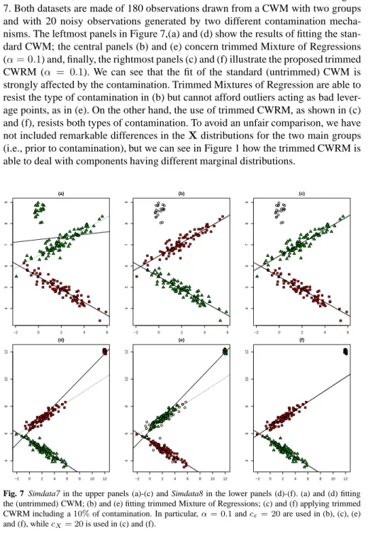
For instance, consider the simulated datasets Simdata7 and Simdata8 in Figure 7. Both datasets are made of 180 observations drawn from a CWM with two groups and with 20 noisy observations generated by two different contamination mecha-nisms. The leftmost panels in Figure 7,(a) and (d) show the results of fitting the stan-dard CWM; the central panels (b) and (e) concern trimmed Mixture of Regressions (α= 0.1) and, finally, the rightmost panels (c) and (f) illustrate the proposed trimmed CWRM (α = 0.1). We can see that the fit of the standard (untrimmed) CWM is strongly affected by the contamination. Trimmed Mixtures of Regression are able to resist the type of contamination in (b) but cannot afford outliers acting as bad lever-age points, as in (e). On the other hand, the use of trimmed CWRM, as shown in (c) and (f), resists both types of contamination. To avoid an unfair comparison, we have not included remarkable differences in theXdistributions for the two main groups (i.e., prior to contamination), but we can see in Figure 1 how the trimmed CWRM is able to deal with components having different marginal distributions.
−2 0 2 4 6
4
5
6
7
8
9
(a)
−2 0 2 4 6
4
5
6
7
8
9
(b)
−2 0 2 4 6
4
5
6
7
8
9
(c)
−2 0 2 4 6 8 10 12
4
6
8
10
12
(d)
−2 0 2 4 6 8 10 12
4
6
8
10
12
(e)
−2 0 2 4 6 8 10 12
4
6
8
10
12
(f)
Fig. 7 Simdata7 in the upper panels (a)-(c) and Simdata8 in the lower panels (d)-(f). (a) and (d) fitting
the (untrimmed) CWM; (b) and (e) fitting trimmed Mixture of Regressions; (c) and (f) applying trimmed CWRM including a10%of contamination. In particular,α= 0.1andcε= 20are used in (b), (c), (e)
and (f), whilecX= 20is used in (c) and (f).
The problem of leverage points has been addressed in Robust Regression by
1992). In the context of clusterwise regression, Garc´ıa-Escudero et al. (2010) pro-posed a “second trimming”, by fixing two trimming parametersα1andα2. Parameter
α1controls the effect of outliers corresponding to large values of(yi−bg′xi−b0g)2
whileα2aims at controlling leverage points corresponding to outlying values onx. However, the distinction between these two types of outliers is not always so clear. On the other hand, the unified handling of outliers provided by the trimmed CWRM si-multaneously deals with both types of outliers. As the probability to belong to a clus-ter is not a fixed value,πg, but depends also on the CWM weightφd(xi,µg,Σg)πg,
trimming acts before on points that lay on the farer contours of equiprobability (i.e. sets of points where the p.d.f. of the mixture takes a constant value) from the clus-ter means. We are assuming that outliers are the points(xi, yi)with lower values of
D(xi, yi;θ), rather than points with greater vertical distances(yi−b′
gxi−b0g)2.
Other alternatives to guard CWM against contamination are based on the con-sideration oft-distributions, instead of normal ones, see Ingrassia et al. (2012). They provide a clear robustness gain with respect to the Gaussian CWM. However, without trimming, one single observation placed in a very remote position can still be very harmful. In fact, we can make some components ofbgto be arbitrarily large or small, just by moving one single observation. A small positive fraction of pointwise contam-ination can be very dangerous too, even when it is not distant from the data. On the other hand, the trimmed CWRM is more resistant to extreme contaminations, because it does not make any assumption about how outliers have been generated. Therefore, rather structured sources of outliers (and clearly not generated from at-distribution) can be handled, too.
Several methods can be also found in the literature aimed at robustifying the Mix-tures of Regressions model. Apart from those based on trimming that have been pre-viously cited, methods based on M-estimation have been proposed in Bai et al. (2012) and extending S-estimation in Bashir and Carter (2012). Song et al. (2014) propose to model the error terms by a Laplace distribution, while Yao et al. (2014) suggest to employ thetdistribution. Although all these methods improve the robustness of the model, they do not model the marginalXdistribution. Therefore, they do not take advantage of this information to detect the different mixture components and hence are not able to cope with outliers both onxand ony, acting as bad leverage points. To overcome this issue, Yao et al. (2014) have recently proposed applying their robust Mixture of Regression after using a trimming procedure (with high breakdown point) which removes clear outliers onx. This initial trimming is unfortunately done with-out considering theY variable, nor the joint distribution in (X, Y), corresponding to the different mixture components. The MCD estimator, considered for this initial trimming, is aimed at working on a single contaminated population and can be trou-blesome for detecting outliers when the data set includes different subpopulations.
5 Real data examples
5.1 Tone data
This data set comes from an experiment in music perception introduced in Cohen (1984) which has been analyzed in many papers concerning Mixtures of Regression, (see, e.g. de Veaux, 1989) and their robust versions (Schlittgen, 2011; Hennig, 2002; Bai et al., 2012; Bashir and Carter, 2012; Song et al., 2014; Yao et al., 2014). This data set is shown in Figure 8(a) and the result of applying the trimmed CWRM in (b). We can see that the two main groups (interval memory judgement and partial matching) can be detected by applying the trimmed CWRM. Furthermore,α= 0.05 allows to detect a fraction of outlying observations, within the partial matching group, exhibiting a clear different behavior.
1.5 2.0 2.5 3.0
1.5
2.0
2.5
3.0
3.5
(a)
Actual tone ratio
P
erceiv
ed tone r
atio
1.5 2.0 2.5 3.0
1.5
2.0
2.5
3.0
3.5
(b)
Actual tone ratio
P
erceiv
ed tone r
atio
Fig. 8 Tone data: (a) Data set; (b) Trimmed CWRM fitting withα= 0.05andcX=cε= 20.
The type of outliers included in this data set are not very harmful and, thus, no dra-matic differences can be expected in terms of the estimated parameters, when using any (robust) Mixture of Regressions approach. So, we will proceed to artificially con-taminate the data and use it as a benchmark for the effects of leverage points added through pointwise contamination. This has been already done by Bai et al. (2012), who introduced a6%of contamination at(0,4), when applying an M-estimation ap-proach. In our case, we will use a more complete contamination scheme by adding 9%of point contamination, placed around points(2.5,5),(6,4),(0,0.5)and(5,2.5), successively. The first location,(2.5,5)is a regression outlier, while the remaining three are leverage points.
Contamination Trimmed CWRM Discarded Trimmed MR Discarded location constants outliers constants outliers
(2.5,5) cX=cε= 1 Yes cε= 1 Yes
cX=cε= 103 No cε= 103 Yes
cX=cε= 1010 No cε= 1010 No
(6,4) cX=cε= 1 Yes cε= 1 No
cX=cε= 103 No cε= 103 No
cX=cε= 1010 No cε= 1010 No
(0,0.5) cX=cε= 1 Yes cε= 1 No
cX=cε= 103 Yes cε= 103 No
cX=cε= 1010 No cε= 1010 No
(5,2.5) cX=cε= 1 Yes cε= 1 No
cX=cε= 103 No cε= 103 No
cX=cε= 1010 No cε= 1010 No
Table 1 Tone data: Performance comparison between the trimmed CWRM methodology and trimmed
Mixture of Regressions (trimmed MR) with anα= 0.1trimming level.
cε, and labeling by “Yes”/“No” the cases in which the trimming level allows/does
not allow to discard all the noisy observations. We can see that only the use of the trimmed CWRM withα= 0.1and with both constants fixed at their most restrictive values is able to cope with the contamination in all the considered scenarios.
5.2 Students’ heights and weights
The data set in this example is based on students answers to a questionnaire including simple questions about anthropometric measurements. Due to the way in which the dataset has been collected, it contains outliers, as some students did not seriously answer the questions, or gave bad interpretations of the measurement units, etc. Here, we focus on the relationship between two variables in the data set, namely “Height” (X) in cm and “Weight” (Y) in Kg. Although gender was also considered in the study, we will ignore it, to test the ability of our methodology to classify the individuals and to estimate the two underlying regression models, one for each gender, in presence of an important amount of severe outliers.
Figure 9(a) shows the original data set (which will be referred to as Student data) with the true gender assignments, while in (b) we have eliminated the points corre-sponding to a wrong scale in height (students reporting height in meters instead of centimeters), to emphasize the different linear patterns. Several implausible weight values can be also seen. Figure 9(c) shows the results corresponding to the fit of the CWM (whenα= 0andcx=cǫ= 1010, i.e., no trimming and almost unrestricted).
obser-0 50 100 150 200
50
100
150
200
(a)
Woman Man Woman Man
160 170 180 190
50
100
150
200
(b)
Woman Man Woman Man
0 50 100 150 200
50
100
150
200
(c)
0 50 100 150 200
50
100
150
200
(e)
160 170 180 190
50
100
150
200
(d)
160 170 180 190
50
100
150
200
(f)
Fig. 9 Student data: (a) “Students’ heights and weights” data. (b) Cleaned data set obtained by deleting the outliers due to wrong measurement scale for “height”. Effects of trimming and restrictions on CRWM results: (c) untrimmed and almost unrestricted:α= 0andcX=cε= 1010; (d) untrimmed and almost unrestricted:α= 0andcX=cε= 1010for the cleaned data set; (e) trimmed and constrained:α= 0.1 andcX=cε= 20; (f) trimmed and constrained:α= 0.04andcX=cε= 20for the cleaned data set
vations is just12%. Figures 9(d) and (f) show the data set after eliminating the points with wrong units for the height. In Figure 9(d), we can see that using the CWM, even in this cleaned data set, again fails to detect the true groups. On the contrary, we can see in (f) that the trimmed CWRM withα = 0.04and moderate values of
served to “clean” this data set but this is surely not the case when dealing with more complex/high dimensional data sets on when carrying out fully unsupervised data analyses.
6 Concluding remarks
The present work is centered on the wide family of Gaussian CWMs, that received a growing attention in the recent literature. However, like it happens for many other models which depend on normal assumptions, the ML estimation for CWM suffers from a lack of robustness. Moreover, the problem statement in terms of the likelihood maximization is not well-posed, without constraints. Hence, here we have presented a new estimation framework for the linear Gaussian CWM based on trimming and constraints, to achieve robustness, identify and discard outliers, circumvent the like-lihood singularities and reduce the detection of spurious solutions.
Numerical studies, based on both simulated and real data, show that the new proposal drives the estimation procedure to discard even strongly concentrated con-taminating observations, acting as bad leverage points, which are so harmful in the framework of Mixtures of Regressions. Apart from the effectiveness of the proposed methodology to resist to any kind of outliers, we have also shown that a theoretically well defined mathematical and statistical problem underlies it. The existence of op-tima for both the population and the sample problem have been established, and the consistency of the sample solution to the population one has been provided.
Further research could be focused on tuning the choice of the involved param-eters. This is a complex task, as these parameters are clearly interrelated. For in-stance, a high trimming levelαcould lead to smallerGvalues, since components with fewer observations may be trimmed off. Moreover, larger values ofcX andcε
could lead to higher values ofG, since more components with few observations, but close to collinearity, may be detected. Our suggestion is that the researcher must provide in advance part of these parameters (as a way of specifying the type of clusters expected from the data) and, then, some data-dependent diagnostic can be used to make appropriate choices for the rest of parameters. The use of trimmed BIC notions (Neykov et al., 2007) or the adaptation of some graphical tools, as in Garc´ıa-Escudero et al. (2011), can be useful for this purpose.
Acknowledgements This research is partially supported by the Spanish Ministerio de Ciencia e
Inno-vacin, grant MTM2011-28657-C02-01, by Consejera de Educacin de la Junta de Castilla y Len, grant VA212U13, and by grant FAR 2013 from the University of Milano-Bicocca.
Appendix
Part A: Preliminary results in view of Proposition 3.2.1
Four technical lemmas will be needed before attacking the proof of Proposition 3.2.1. First of all, let us remark that, given the definition ofL(θ, P), there exist se-quences{θn}∞
n=1with
θn= (π1n, ..., πGn,µn1, ...,µnG,Σ n
1, ...,ΣnG, b
0,n
1 , ..., b 0,n
G ,bn1, ...,bnG, σ
2,n
1 , ..., σ 2,n G ),
(11) andθn∈ΘcX,cεand such that
lim
n→∞L(θn, P) = sup
θ∈ΘcX ,cε
L(θ, P)>−∞ (12)
(the boundedness from below is obtained just by considering the setAas being a ball centered at(0,0)withP[A] ≥1−α,π1 = 1,µ1 =0,Σ1 =Id,b01 = 0and b1=0).
The proof of the existence will be done by proving that we can obtain a convergent subsequence extracted from{θn}∞
n=1satisfying (12), and whose limitθ0is optimal forP.
Let us begin with Lemma 1, which provides a uniformly bounded representation of the regression coefficients, even in case of local collinearity, without loosing their properties in the evaluation of the target function.
Lemma 1 Let {b0
n}∞n=1 be a sequence in R, {bn}∞n=1 be a sequence in Rd and
{An}∞
n=1be a sequence of sets inRd+1verifying
lim sup
n
P[An]>0 (13)
and such that
lim sup
n EP
|b0n+b′nX−Y|2IAn(X, Y)
<∞. (14)
Then, we can extract subsequences{b0
nk}
∞
k=1,{bnk}
∞
k=1and{Ank}
∞
k=1from them and define new sequences{d0
k}∞k=1,{dk}∞k=1and{Dk}∞k=1which satisfyDk ⊆Ank,
P[Ank\Dk]→0,d
0
nk →d
0∈R,d
nk →d∈R
dand such that
(b0nk+b′
nkX−Y)IDk(X, Y) = (d
0
k+d
′
kX−Y)IDk(X, Y), P-a.s., (15)
for everyk≥1.
Proof:To simplify the proof, w.l.o.g., we will use the same notation for the sub-sequences as that used for the original sub-sequences. If the sub-sequences {b0
n}∞n=1 and
{bn}∞
n=1are bounded, then we just need to extract convergent subsequences and set
Dn =An. So, let us assume that either one or both sequences are unbounded, and
consider a sequence of compact sets{Kn}∞n=1such thatKn↑Rd+1. Let{vnl}
d l=1be the normalized eigenvectors obtained from the spectral decomposition of the matrices
Now, let us suppose that there exists a directionvn
lsuch that VarP[v
′
nlX/An∩
Kn]→ 0then takeH with0 ≤H < dand such that VarP[v′nlX/An∩Kn]→ 0
for everyl ≥ H + 1, after a possible reordering of the coordinates. In this case, there also exist points{un
l}
d
l=H+1inRdand a sequenceεn↓ 0which must satisfy EP[|vn′l(X−unl)|> εn/An∩Kn]→0for everyl≥H+ 1. Thevnlare bounded
(unitary vectors) and theun
lmust be bounded too (because, otherwise,Xwould not
be tight). Therefore, there exist subsequences, that will be denoted as the original ones, such thatvn
l → vl ∈ R
d,u
nl →ul ∈R
d andP[|v′
l(X−ul)| > 0/An∩ Kn]→0for everyl≥H+ 1.
Let us now defineDn =An∩Kn∩dl=H+1{v′l(X−ul) = 0}which trivially
verifiesDn⊂Anand thatP[An\Dn]→0. We can rewrite
b0n+b′nx=b0n+ H
X
l=1
b′nvlv′lx+
d
X
l=H+1
b′nvlv′lx.
and setd0
n=b0n+
Pd
l=H+1b′nulanddn =PHl=1b′nvlv′lforH >0(while we set
dn =0whenH = 0). Then (15) trivially holds and it can be shown that{d0
n}∞n=1 and{dn}∞
n=1are bounded sequences. This follows from the fact that (14) guarantees that{(b0
n+b′nX−Y)IDn(X, Y)}
∞
n=1is a tight sequence. Notice that we could see that the previous tightness property would be contradicted if any of the{d0
n}∞n=1and
{dn}∞
n=1were unbounded by seeing thatZ= (Z1, ..., ZH)withZl=v′lxsatisfies
det(VarP[Z/An∩Kn])>0andd′nx=
PH
l=1b′nvlZl.
Finally, whenever none of the sequences VarP[v′nlX/An∩Kn]converges to 0,
we can consider the representationb0
n+b′nx=b0n+
PH
l=1b′nvlv′lxand the result
would be proven in this case, too, following similar arguments as before.✷
The following Lemma 2 assures that, under the usual assumption onP, the as-sociated fitted trimmed CWMs could not be arbitrarily close to a degenerated model concentrated onGpoints, nor onGregression hyperplanes.
Lemma 2 LetPbe a distribution inRd+1satisfiying (PR):
(a) For everyb0
g∈R,bg∈RdandA⊆Rd+1withP[A] = 1−α, there existsδ >0
such that
EP
min
g=1,...,G|b
0
g+b
′
gX−Y|
2I
A(X, Y)
≥δ.
(b) For every set ofGpoints{µ1, ...,µG} ⊂RdandA⊆Rd+1withP[A] = 1−α, there existsδ >0such that
EP
min
g=1,...,Gk
X−µgk2IA(X, Y)
≥δ.
Proof of (a):Let us suppose thatδdoes not exist. Then, we can choose sequences
{An}∞
n=1,{b0g,n}∞n=1and{bng}∞n=1such that
EP
min
g=1,...,G|b
0,n g + (bng)
′x−y|2I
An(x, y)
Moreover, we can replace the setsAnin (16), by the data sets
A∗n=
(x, y) : min
g=1,...,G|b
0,n
g + (bng)′x−y|2≤min{rnα, ε} ,
wherern
α = infu{P[(x, y) : ming=1,...,G|b0g,n+ (bng)′x−y|2 ≤u]≥1−α}and
we also have the same convergence as in (16), withP[A∗
n] → 1−αfor any fixed
choice ofε >0. Then, take
Ang =
(x, y)∈A∗
n:|b0g,n+ (bng)′x−y|= min j=1,...,G|b
0,n
j + (bnj)′x−y|
,
and, we can see that there exists at least onegsuch thatP[An
g] →pg > 0through
a subsequence (becauseP[A∗
n] =
P
g=1,...,GP[Ang] → 1−α). Thus, consider a
reordering of{1, ..., G}such thatP[An
g]→pg >0for everyg∈ {1, ..., H}(for an
appropriate subsequence, if needed). IfA∗∗
n =∪Hg=1Ang, then
EP
min
g=1,...,G|b
0,n
g + (bng)′X−Y|2IA∗∗
n(X, Y)
= H X g=1 EP
|b0,n
g + (bng)′X−Y|2IAn
g(X, Y)
andP[A∗∗
n ] → 1−α. For everyg ∈ {1, ..., H}, theAng,b0g,n andbng satisfy the
conditions needed to apply Lemma 1 and, therefore, we can replace them byDn g,d0g,n
anddn
g satisfyingDgn⊂Ang,P[Ang\Dgn]→0,d0g,n→d0g∈Randdng →d0g∈Rd
and (15).
Now, takeBn =∪g=1,...,HDgn∩ {(x, y) : ming=1,...,G|d0g,n+ (dng)′x−y|2≤ε}
for a fixedε, withP[Bn]→1−α. We thus have the pointwise convergence
min
g=1,...,H|d
0,n g + (dng)
′x−y|2I
Bn(x, y)→ min
g=1,...,H|d
0
g+ (d
0
g)
′x−y|2I
B0(x, y),
for anyB0⊂Rd+1withP[B0] = 1−α, and the uniform boundming=1,...,H|d0g,n+
(dng)′X−Y|2IB
n(x, y)≤ε.Then, the dominated convergence theorem implies
Ep
min
g=1,...,H|d
0,n
g + (dng)′X−Y|2IBn(X, Y)
→Ep
min
g=1,...,H|d
0
g+ (d
0
g)
′X−Y|2I
B0(X, Y)
.
The latter convergence and (16) would prove that
Ep
min
g=1,...,H|d
0
g+ (d0g)′X−Y|2IB0(X, Y)
= 0,
Proof of (b):The proof of this results mimics the steps followed in the proof of (a). We start by assuming the existence of subsequences{An}∞
n=1 and{µng}∞n=1 such that
EP
min
g=1,...,Gk
x−µn
gk
2I
An(x, y)
→0withP[An]→1−α.
and we would end up by seeing that the supportXis concentrated inGpoints inRd. In fact, the proof is easier because only the tightness ofPis needed (Lemma 1 is no longer required, here).✷
Now, since [0,1]G is a compact set, we can trivially choose a subsequence of {θn}∞
n=1 such thatπng → πg ∈ [0,1]for1 ≤ g ≤ G.With respect to the scatter
matrices and the variances of the error terms, we have the following possibilities:
(S1)Σng →Σgfor1≤g≤GwithΣgbeing p.s.d. matrices
(S2) min
g=1,...,Gl=1min,...,dλl(Σ n g)→ ∞
(S3) max
g=1,...,Gl=1max,...,dλl(Σ n g)→0
(V1)σ2g,n→σ2gfor1≤g≤Gwithσg>0
(V2) min
g=1,...,Gσ
2,n
g → ∞
(V3) max
g=1,...,Gσ
2,n g →0
Given thatθn∈ΘcX,cε, only one of the convergences in S1-S3 and only one in
V1-V3 are possible, and the following Lemma 3 will further delimitate to the bounded results, based on constraints (5) and (6).
Lemma 3 If{θn}∞
n=1 ⊂ ΘcX,cε converges toward the supremum ofL(θ, P), and
(PR) holds forP, then only convergences (S1) and (V1) are possible.
Proof:We have thatL(θn;P)can be bounded from above by
−1 2 " log min g σ 2,n g
P[A(θn)] +
EPming|b0g,n+ (bng)′X−Y|2IA(θn)(
X, Y)
maxgσ2g,n
# −1 2 " log min
g minl λl(Σ n g)
P[A(θn)]d+ EP
mingkX−µngk2IA(θn)(X, Y)
maxgmaxlλl(Σng)
#
+C,
whereCis a constant value, not depending onθn.
Therefore, given that θn ∈ ΘcX,cε, we see that the possible convergence of
L(θn;P)would clearly depend on those for the sequences
log σ2 n cε
P[A(θn)] +EP
min
g
b0,n
g + (bng)′X−Y
2
IA(θ
n)(
X, Y)
1 σ2 n (17) and log λn cX
P[A(θn)]d+EP
min
g k
X−µn
gk
2I
A(θn)(
X, Y)
1
λn
whereλn= maxg=1,...,Gmaxl=1,...,dλl(Σng)andσn2= maxg=1,...,Gσg2,n.
On the other hand, Lemma 2 implies that a constantδ >0can be chosen such that
EP
ming|b0g,n+(bng)′X−Y|2IAn(X, Y)
andEP
mingkX−µgk2IAn(X, Y)
in (17) and (18) are uniformly bounded from below byδ. Therefore, other convergences different from (S1) or (V1) would imply thatlimn→∞L(θn, P) = −∞and this
would contradict (12).✷
Lemma 4, stated below, shows that we can always find a subsequence{θn}∞
n=1 with converging parameters for at least one mixture component, with weightπn
g
con-verging toward a strictly positive value.
Lemma 4 There exists a sequence {θn}∞
n=1 converging toward the supremum of
L(θ, P)and there existsH with1≤H≤Gsuch that
µgn→µg, bg0,n→b0g, bng →bg and πng →πg>0 for every g≤H
and such that the corresponding{A(θn)}∞n=1sets are uniformly bounded.
Proof:Let us start from any{θn}∞n=1converging toward the supremum ofL(θ, P), and takeAn=A(θn)and
An g =
(x, y)∈An :Dg(x, y;θ) = max
j=1,...,GDj(
x, y;θ)
for1 ≤ g ≤ G. SinceP[An
g] ∈ [0,1], there exists a subsequence, denoted as the
original one, such that eachP[An
g]converges for1≤g≤G. Moreover, after a proper
reordering in the components ofθn, there existsH∗≥1such thatP[Ang]→pg>0
for1 ≤ g ≤ H∗. Note that this H∗ does exist because otherwise we would have
P[An] =PGg=1P[Ang]→0.
We can also find a convergent subsequence ofµng for everyg≤H∗. Otherwise,
for everyηwith0< η < pg, we could take a ballBgcentered at(0,0)withP[Bg]>
1−pg+η and such that there existsn0withP[Bg∩Ang] > η/2whenn ≥ n0.
Consequently, we would haveEP
kX−µn gk2IAn
g
≥EP
kX−µn
gk2IBg∩Ang
→ ∞
which contradicts (12). Note that the contributions of the other terms toL(θn, P)are
controlled, because of Lemma 3.
From (12), we havelim supnEP|b0g,n+ (bng)′X−Y|2IAn
g(X, Y)
<∞. This, together with the fact thatlim supnP[An
g] =pg>0forg≤H∗, allows us to apply
again Lemma 1 to replace the {b0,n
g },{bng} and{Ang} sequences by appropriated
convergent sequences{d0,n
g },{dng}and{Dng}. These convergences also trivially
im-ply thatπn
g →πg>0forg≤H∗.
Othergvalues could also satisfy these convergences (through subsequences and possible alternative representations). In this case, we considerH ≥H∗such that all the convergences in the statement of this Lemma hold forg≤H.
To see that the{A(θn)}∞n=1are uniformly bounded, recall thatA(θn) ={(x, y) : D(x, y;θn)≥R(θn, P)}and let us introduce
e
R(θn, P) = sup u
P
max 1≤g≤HDg(
X, Y;θn)≥u
≥1−α
.
Given thatD(x, y;θn)≥maxgDg(x, y;θn), we trivially have the boundRe(θn, P)≤
R(θn, P). Moreover,πgn,µng,Σ n
H and, then, we can also find a strictly positive constantRHsatisfying0 < RH ≤
e
R(θn, P)≤R(θn, P).The setsBn={(x, y) : maxg≤HDg(x, y;θn)≥RH}
sat-isfy thatAn ⊆Bnand all theseBnsets are uniformly bounded just by taking into
ac-count the uniform continuity of the set functions{(x, y)7→maxg≤HDg(x, y;θn)}∞n=1 and that the parameters corresponding to the firstHgroups in{θn}∞
n=1are uniformly bounded.✷
Having established these crucial findings, we are ready to prove the existence result.
Part B: Proof of Proposition 3.2.1
Let us start from a sequence{θn}∞
n=1converging toward the supremum ofL(θ, P). Thanks to Lemma 2, we know that there exists a subsequence of {θn}∞n=1 with
Σng → Σg andσ2g,n → σ2g for1 ≤ g ≤ G. Moreover, by applying Lemma 4, a
further subsequence (with a proper modification, if needed) can be obtained that also verifiesµn
g →µg, b0g,n →b0g,bng →bgandπng →πg withπg >0for anygwith g ≤ H and1 < H ≤ G. Let us assume that there exists somegsuch thatµn
g is
not bounded, or such that a bounded representation forb0,n
g andbng(in the sense that
lim supnEP
|b0,n
g + (bng)′X−Y|2IAn(X, Y)] = ∞) does not exist. We will see
that we necessarily must have thatπn
g → 0 and, consequently, the role played by µn
g, b0g,nandbng is irrelevant, given that they do not modify the value taken by the
target function. Therefore, we could modify them by using other arbitrary convergent parameter values (of course, satisfying the desired constraints) and the proof would be done.
To prove that, let us consider
Mn=EP
"
log
XG
g=1
Dg(X, Y;θn)
−log
XH
g=1
Dg(X, Y;θn)
!
IAn(X, Y) #
.
By considering the sameRH > 0 used in the proof of Lemma 4 and the fact that
log(1 +x)≤x, we can see that
Mn≤ G
X
g=H+1
EP
Dg(X, Y;θn) RH
IAn(X, Y)
.
Then, it is trivial to see thatMn →0whenµng is not bounded or when no bounded
representation forb0,n
g andbng exists for anyg > H. Consequently, ifπgn→πg >0
for anyg > Handθ∗is the limit of the subsequence{πn
1, ..., πHn,µn1, ...,µnH,Σ n
1, ...,ΣnH, b01,n, ..., b0H,n,bn
1, ...,bnH, σ
2,n
1 , ..., σ 2,n H }
∞
n=1, we would have thatlimn→∞supL(θn;P)
=L(θ∗;P)(becauseMn →0) withPHj=1πj<1. Then, we could define a new
sub-sequence{θen}∞
n=1={π˜n1, ...,π˜nG,µ˜ n
1, ...,µ˜nG,Σ˜ n
1, ...,Σ˜
n G,˜b
0,n
1 , ...,˜b 0,n
G ,b˜n1, ...,b˜nG,
˜
σ12,n, ...,σ˜ 2,n
G }∞n=1with
e
πng = πn
g
Pk
g=1πnj
withµeng =µn
g,eb0g,n =b0g,n,beng =bng,Σe n
g =Σng andσe2g,n =σ2g,nfor1≤g ≤H
and parameters arbitrarily chosen wheng > H (only satisfying the required con-straints). We finally could see thatlimn→∞supL(θen;P)<limn→∞supL(θn;P)
and this would contradict the optimality stated in the hypothesis of the present lemma.
✷
Part C: Preliminary results in view of Proposition 3.2.2
Before starting the proof of the consistency of the solution for the sample problem to the population solution, we introduce some notation, and state some useful results. Let{θˆn}∞
n=1={πˆn1, ...,πˆnG,µˆ n
1, ...,µˆ
n G,Σˆ
n
1, ...,Σˆ
n G,ˆb
0,n
1 , ...,ˆb 0,n
G ,bˆn1, ...,bˆnG,σˆ
2,n
1 , ..., ˆ
σG2,n}∞
n=1 ⊂ΘcX,cε denote a sequence of empirical estimators obtained by solving
the empirical problems defined from the sequence of empirical measures{Pn}∞n=1. First, we prove that there exists a compact setK⊂ΘcX,cεsuch thatθˆn ∈Kwith
probability 1. This is done through Lemmas 5 and 6, whose proofs are quite straight-forward adaptations of the previously given proofs of Lemmas 1, 2, 3 and 4. In those adaptations, appropriate Glivenko-Cantelli class of functions must be considered and the class of balls inRd+1(which is a Glivenko-Cantelli class too) is taken to provide bounding compact sets when needed.
Lemma 5 IfP satisfies (PR), then only convergences (S1) and (V1) are possible for theΣˆng’s andσˆ2,n
g ’s.
Lemma 6 If (PR) holds, then we can choose a sequence{θˆn}∞
n=1solving the empir-ical problem with componentsµˆng,ˆb0,n
g andbˆng such that their norms are uniformly
bounded.
The following two lemmas are the analogous to Lemmas 5 and 6 in Garc´ıa-Escudero et al. (2014b). Their proofs mimic the same steps, with the only reformulation of the
D(·;θ)functions, which here take into account the conditional distribution on the
Y variable.
Lemma 7 Given a compact setK⊂ΘcX,cε,B⊂R
d+1and[a, b]⊂R, the class of
functions
H:=
IB(·)I[u,∞) D(·,θ)
log(D(·;θ)) :θ∈K, u∈[a, b]
(19)
is a Glivenko-Cantelli class.
Lemma 8 LetP be an absolutely continuous distribution with strictly positive den-sity function. Then, for every compact setK, we have that
sup
θ∈K
|R(θ, Pn)−R(θ, P)| →0, P-a.e. .
In fact, the condition on the existence of a strictly positive density function forP
Part D: Proof of Proposition 3.2.2
Taking into account Lemma 7, the consistency follows from Corollary 3.2.3 in van der Vaart and Wellner (1996), exactly as it was done in Garc´ıa-Escudero et al. (2008) and in Garc´ıa-Escudero et al.
(2014b). Note that Lemmas 5 and 6 guarantee the existence of a compact set K
such that {θˆn}∞
n=1 is included inK with probability 1 andR(ˆθn, Pn) is also
in-cluded with probability 1 within an interval[a, b] due to Lemma 8. This has been also used to simplify the target function needed to apply the aforementioned result in van der Vaart and Wellner (1996).
References
Bai, X., Yao, W., Boyer, J., 2012, Robust fitting of mixture regression models, Com-put. Stat. Data Anal., 56 (7), 2347–2359.
Bashir, S., Carter, E., 2012, Robust mixture of linear regression models, Comm. Stat.-Theory and Methods, 41 (18), 3371–3388.
Cohen, E., 1984, Some effects on inharmonic partials on interval perception, Music Percept., 1 (3), 323–349.
Cuesta-Albertos, J.A, Gordaliza, A., Matr´an, C., 1997, Trimmedk-means: an attempt to robustify quantizers, Ann. Stat., 25 (2), 553–576.
Dasgupta, A., Raftery, A.E., 1998, Detecting features in spatial point processes with clutter via model-based clustering, J. American Stat. Assoc., 93 (441), 209–302. Day, N., 1969, Estimating the components of a mixture of normal distributions,
Biometrika, 56 (3), 463–474.
de Veaux, R., 1989, Mixtures of linear regressions, Comput. Stat. Data Anal., 8 (3), 227–245.
DeSarbo, W., Cron, W., 1988, A maximum likelihood methodology for clusterwise linear regression, J. Classification, 5 (2), 249–282.
Fritz, H., Garc´ıa-Escudero, L., Mayo-Iscar, A., 2013, A fast algorithm for robust constrained clustering, Comput. Stat. Data Anal., 61, 124–136.
Gallegos, M., Ritter, G., 2009, Trimmed ML estimation of contaminated mixtures, Sankhya (Ser. A), 71, 164–220.
Garc´ıa-Escudero, L., Gordaliza, A., Matr´an, C., Mayo-Iscar, A., 2014a, Avoiding spurious local maximizers in mixture modelling, doi 10.1007/s11222-014-9455-3, forthcoming inStat. Comput..
Garc´ıa-Escudero, L., Gordaliza, A., Mayo-Iscar, A., 2014b, A constrained robust proposal for mixture modeling avoiding spurious solutions, Advances Data Anal. Classification, 8 (1), 27–43.
Garc´ıa-Escudero, L., Gordaliza, A., San Mart´ın, R., Mayo-Iscar, A., 2010, Robust clusterwise linear regression through trimming, Comput. Stat. Data Anal., 54 (12), 3057–3069.