A solution to the transfer princing problem by successively reducing the duality gap

Texto completo

(1)107. A SOLUTION TO THE TRANSFER PRINCING PROBLEM BY SUCCESSIVELY REDUCING THE DUALITY GAP. Carlos J. Vidal Holguín Profesor Titular. Universidad del Valle. Escuela de Ingeniería Industrial y Estadística, Cali cjvidal@univalle.edu.co. Marc Goestschalckx School of Industrial and Systems Engineering, Georgia Institute of Technology, Atlanta, USA marc.goetschalckx@isye.gatech.edu. Abstract We consider the model by Vidal and Goetschalckx (2001) and implement a global optimization procedure to configure a global supply chain in order to maximize the after tax profits, including transfer prices and the allocation of transportation costs as explicit decision variables. The resulting mathematical formulation is a non-convex optimization problem with a linear objective function, a set of linear constraints, and a set of bilinear constraints. We implement a global optimization procedure based on the results by Ben-Tal et al. (1994), which successively reduces the duality gap and thus we can obtain εoptimal solutions in reasonable computation time. Our results show that the procedure can obtain near-optimal solutions within a gap less than one percent of the upper bound in satisfactory computation time for all the instances that we considered. We also illustrate the potential benefits that companies may achieve when applying the model and its solution procedures through several computational experiments. Keywords: Transfer Pricing; Global supply chain optimization; Global Optimization; Production/Distribution Models.. Resumen Consideramos el modelo de Vidal y Goetschalckx (2001) e implementamos un procedimiento de optimización global para configurar una cadena de abastecimiento global con el objeto de maximizar las utilidades después de impuestos, incluyendo precios de transferencia y la asignación de costos de transporte como variables explícitas de decisión. La formulación matemática resultante es un problema de optimización no convexo con una función objetivo lineal, un conjunto de restricciones lineales y un conjunto de restricciones bilineales. Se implementa un procedimiento de optimización global basado en los resultados de Ben-Tal et al. (1994), el cual reduce sucesivamente la brecha dual y así se obtienen soluciones εóptimas en un tiempo de computación razonable. Nuestros resultados muestran que el procedimiento puede encontrar soluciones aproximadamente óptimas con brechas menores que el 1% del límite superior en tiempos de computación razonables para todos los casos resueltos. Ilustramos igualmente los beneficios potenciales que las empresas podrían lograr al aplicar el modelo y la técnica de solución desarrollada mediante varios experimentos computacionales. Palabras clave: Precios de transferencia; Optimización de cadenas de abastecimiento globales; Optimización global; Modelos de Producción/Distribución..

(2) 108. 1. Introduction A transfer price is the price that a selling department, division, or subsidiary of a company charges for a product or service supplied to a buying department, division, or subsidiary of the same firm [Abdallah (1989)]. O’Connor (1997) states that, “Transfer pricing is the most important international tax issue facing multinationals today, and is expected to remain so for the near future.” In his survey of over 200 multinational companies (MNCs), 80 percent of them identified Transfer Pricing (TP) as the number one issue they have to face. Abdallah (2004) expresses that for the last 30 years, all MNCs have experienced no business function that goes so deeply into nearly all business operations as international TP. Abdallah mentions that TP decisions have a significant impact on all the operations and management of an international company, even affecting the ability of the company to accomplish its fundamental objectives. Moreover, he claims that “TP is considered one of the most important as well as most complicated business issues in the world.” More recently, Rosenthal (2008) says that the TP problem has been of interest to managers, accountants, and economists for a long time. TP is therefore one of the most controversial topics for MNCs. The problem is to find transfer prices so that the global corporate goals are satisfied and the performance measures are fair for all the firm’s subsidiaries and divisions. According to O’Connor (1997), the problem originates from the conflicts between the goals of the global corporation and the goals of its subsidiaries, and from the constraints imposed by the legal environment involving taxes and tariffs. The utilization of the arm’s length principle, which establishes the use of transfer prices as if the involved parties did not belong to the same corporation, is widely accepted. Accordingly, Gernon and Meek (2000) say that most TP policies are based on either external market prices or internal costs. Both have the advantage of being acceptable to tax authorities. MNCs seek diverse objectives when setting their transfer prices. O’Connor (1997) presents the results of several surveys concerning the key goals that MNCs try to achieve through their TP. policies. Generally, the results of these surveys are not consistent since some of them give more importance to some objectives, whereas others disregard the same goals. In summary, these objectives, which continue to be pertinent nowadays, are to: • • • • • • •. Satisfy tax and other legal requirements; Produce profit maximization by minimizing worldwide taxes and duties; Produce a fair framework for performance evaluation and motivation of all related parties; Move funds internationally; Minimize exchange rate risk; Avoid exchange controls and quotas; and Increase profit share from joint ventures.. One of the most controversial objectives of TP policies is profit maximization by minimizing worldwide taxes and duties. O’Connor (1997) remarks that although many companies argue that tax minimization is not their main goal, in reality many firms appear to design TP policies to take advantage of differential tax structures among countries. In spite of the current regulations imposed by most countries intended to avoid the arbitrary manipulation of transfer prices, there exist significant opportunities for profit maximization that are not illegal. Very likely, the flexibility is decreasing each day, but the impact of small changes in transfer prices on the global profit of a company may be substantial. Therefore, designing TP policies to minimize taxes legally should not be ignored by MNCs that prefer to design policies consistent with the corporate strategy and organizational structure of the company. Most global supply chain literature has addressed TP as an accounting topic rather than an important global supply chain planning problem [Miller and de Matta (2008)]. The TP problem is much more than an accounting problem; it is indeed a fundamental supply chain planning problem and a decision opportunity that significantly affects the design and management of a global supply chain or a local one when regional taxes vary significantly. In general, when a logistics analyst attempts to determine the optimal flows of raw materials and products among facilities, the prices.

(3) 109. of raw materials and products are almost always considered as fixed and given parameters. Consequently, most models that address the TP problem do not include transfer prices as explicit decision variables. However, this is not the case in real global logistics systems since management can determine the transfer prices with some degree of flexibility. According to Stitt (1995), the Organization for the Economic Cooperation and Development (OECD) defines a range of an acceptable transfer price rather than a single, ‘correct’ transfer price. For example, transfer prices can be determined from given lower and upper bounds, or based on the total or variable production cost. Abdallah (1989) comments on the difficulty of using market prices as the selected TP policy in an international environment, mainly because of the diversity of economic environments and transportation costs. Moreover, there will always exist a tradeoff between the low transfer price desired by the buyer division and the high transfer price desired by the seller division. Abdallah (2004) remarks that making TP decisions for MNCs have a great impact on their global operations, directly affecting their revenues and profits and all their functions, such as manufacturing, marketing, management, and financing. Several researchers have addressed the TP problem as an integral component for the optimization of a global supply chain. Nieckels (1976) presents a nonlinear mathematical model to determine optimal transfer prices and resource allocation in a multinational textile firm. Although this formulation includes transfer prices as decision variables and a linear objective function for maximizing the global net income after taxes, the author does not address the decision of allocating transportation costs since they are always charged to the destination subsidiary. Although Nieckels says that small changes in transfer prices may lead to significant differences in the after-tax profit of a company, he does not attempt to calculate upper bounds to test the performance of the primal heuristic method he develops. Cohen et al. (1989) present a formulation of a normative global supply chain model that is a dynamic, nonlinear, mixed integer programming. formulation that considers transfer prices as decision variables. No computational experience is presented in this paper, but the authors state that they and other researchers have successfully developed some variants of the model. One of these is the work by Cohen and Lee (1989), which describe a single-period multi-commodity model that analyzes resource deployment decisions in a personal computer manufacturer. This model considers the decision of allocating transportation costs to either the origin or the destination by formulating binary variables. However, in the presented solution process, this decision is made externally and the corresponding binary variables are fixed in advance. Vidal (1998) and Vidal and Goetschalckx (2001) formulate a global supply chain optimization model and present a successive LP solution procedure for solving the TP problem. By reformulating some of the variables in the model, the authors develop an upper bound that can be determined by solving a linear program. They implement an iterative procedure that switches between fixing either the transfer prices or the flows, and solving the remaining LP problem, until no further improvement in the objective function is possible. The instances tested with this LP-based primal heuristic yield gaps within one percent of optimality in less than 200 seconds of computation time on average. The global optimization procedure described in this paper uses this heuristic as an embedded subroutine to determine feasible solutions. In a further review, Goetschalckx et al. (2002) concentrate on the savings potential from formulating production/distribution models and TP decisions. They describe the main results given in Vidal and Goetschalckx (2001) and introduce some results of the global optimization procedure fully described in this paper. Several authors have considered the transfer pricing problem as an integral part of global supply chain models, but transfer prices are not included in the formulations as explicit decision variables. In these cases, transfer prices are either fixed in advance or calculated independently of the model. See, for example, Canel and Khumawala (1997), Fandel and Stammen (2004), Lakhal (2006), Vila et al. (2006), Ulstein et al. (2006), and Meijboom and Obel (2007)..

(4) 110. Other researchers have included transfer prices as explicit decision variables in their models, but they have not applied global optimization procedures to solve the problems. Wilhelm et al. (2005) formulate a model to maximize global after-tax profit of a company. They consider transfer prices as decision variables, but allowing them to be different for the same product when it is sent from a location to different destinations. This approach leads to a model that can be linearized and thus it is easier to solve without using global optimization procedures. Villegas and Ouenniche (2008) present a non-linear unconstrained optimization model to understand TP, trade quantity decisions, and transportation cost allocations. This model is not empirically tested and no solution approach is presented, according to the authors, because such a procedure would require more information about cost and revenue functions used in the model. The authors explain that this was deliberately done to keep the model more general. Therefore, no global optimization procedure is applied in this paper. Miller and de Matta (2008) present a nonlinear programming model to maximize global supply chain profits. They transform the model into an approximate linear formulation by stating some assumptions about the system under study. No global optimization procedure is applied to solve the original model. According to Killian (2006), “there is evidence that multinational firms may manage earnings, set transfer prices, or relocate facilities in response to tax changes and incentives. The impact that these actions have on the environment in which they operate, and the jurisdiction they choose to vacate, has not yet been extensively studied.” Based on the work by Ben-Tal et al. (1994), Vidal (1998), Vidal and Goetschalckx (2001), and Goetschalckx et al. (2002), this paper presents a new approach to the TP problem based on a global optimization procedure that successively reduces the duality gap. To the best of our knowledge, no paper before has considered transfer prices and transportation cost allocation as explicit decision variables and has addressed the TP problem by applying global optimization procedures. Our results indicate that MNCs and regional companies operating in. countries where local taxes differ considerably may significantly increase profits by considering the TP problem as a part of the supply chain optimization problem and solving the model by global optimization procedures that can find εoptimal solutions in reasonable computation time. The remainder of this paper is organized as follows. In Section 2 we present a summary of the model and the general problem structure. The global optimization procedure is presented in Section 3, and in Section 4 we illustrate the solution approach with several computational experiments. Finally, Section 5 contains the conclusions of the paper.. 2. Model Summary and General Structure of the Problem 2.1. Original Model Vidal (1998) and Vidal and Goetschalckx (2001) developed the global supply chain model considered in this paper. Figure 1 illustrates the system under consideration. The suppliers are classified into two groups: internal suppliers and external suppliers. For the external suppliers there is no possible decision with respect to transfer prices since they sell directly to the company using market prices. For the internal suppliers a set of optimal transfer prices for the period under consideration is to be determined by the model. The manufacturing plants receive components and raw materials from the suppliers, and perform assembly operations to obtain finished products. Then, the plants send finished products to DCs using a second set of transfer prices, which also is to be determined by the model. Finally, the finished products are distributed worldwide from the DCs to retailers and/or final customers. The main assumptions of the model are the following: •. All internal suppliers, plants, and DCs are considered to be subsidiaries of the parent company and are supposed to be actively involved in manufacturing, selling, shipping, and/or servicing activities..

(5) 111. W Country 2 S. S. C. W. C. M. W. C. M. W. Country 1 S S. C C. Country 3 Country 4. C. S = Suppliers M = Manufacturing Plants W = Distribution Centers C = Customers. Figure 1. Global supply chain under analysis. • • •. •. •. As a consequence, each internal supplier, plant, and DC are assumed to be taxed on their local-source income since the company attempts to maximize the total profit after tax in all the countries where it operates, but no income is remitted as a dividend to the shareholders, and therefore the parent company is only taxed on its local income. TP decisions are centralized. No location decisions are included in the model. All transfer-price variables have a lower and an upper bound, which reflect the feasible markups for production costs and a profit margin or possible discounts on market prices. In this paper, the transfer price, also called ‘basic’ transfer price, is considered to be independent of the transportation cost. The allocation of transportation costs reflects the terms of the transaction, which are more precisely defined by selected INCOTERMS (FOB or CIF, for example). The allocation of the transportation cost to the origin or destination is a decision variable that is considered independently of the transfer price. As a requirement for the justification of transfer prices to tax authorities, all the transfer prices (without including transportation costs) from a given origin and for a given component (or finished product) must be the same for all destinations.. •. •. •. Import duties are paid by the importing country, based on the FOB or CIF value of the transferred products, as appropriated. No export duties are considered. The own supply chain of internal suppliers is not considered. Instead, variable and fixed costs of internal suppliers are included to determine their corresponding profit. There are no significant fluctuations in inventory balance over the period under consideration. The model considers pipeline inventory costs, cycle inventory costs, and safety stock inventory costs to determine the best transportation mode to use on each link. See Vidal and Goetschalckx (2000) for a detailed description of each of the inventory expressions included in the analysis.. In what follows, we present the complete model. Sets and Indexes C= C(k) = M= Mc=. Set of market zones, indexed by l Set of market zones that can be served by DC k ∈ W Set of manufacturing plants, indexed by j Set of manufacturing plants located in countries where duties are charged on the CIF value of imported products; M c⊆ M.

(6) 112. Mf=. M(p) =. M(i) =. P= P(j) = P(r) = R=. R(i) = R(j) = S= S′ =. S ′ (j) = S ′′ = S ′′ (j) =. S(r) = T= T(i, j) =. T(j, k) =. T(k, l) =. W= W(l) =. Set of manufacturing plants located in countries where duties are charged on the FOB value of imported products; M f ⊆ M, M c∪ M f = M, M c∩ M f = φ Set of manufacturing plants that can produce finished product p ∈ P ; M(p) ⊆M Set of manufacturing plants that use at least one raw material provided by supplier i ∈ S; M(i) ⊆ M Set of finished products, indexed by p Set of products that can be produced in manufacturing plant j; P(j) ⊆ P Set of products that use r ∈ R as a raw material; P(r) ⊆ P Set of raw materials, parts or components (called “raw materials”), indexed by r Set of raw materials that can be supplied by supplier i∈ S; R(i) ⊆ R Set of raw materials that plant j ∈ M may need; R(j) ⊆ R Set of suppliers, indexed by i; Set of internal suppliers of the company; S ′ ⊆ S Set of internal suppliers that may send at least one raw material to plant j ∈ M; S ′ (j)⊆ S ′ Set of external suppliers; S ′′ ⊆ S, S ′ ∩ S ′′ = φ, S ′ ∪ S ′′ = S Set of external suppliers that may send at least one raw material to plant j ∈ M; S ′′ (j) ⊆ S ′′ Set of suppliers that can supply raw material r ∈ R ; S(r) ⊆ S Set of transportation modes, indexed by m Set of available transportation modes between supplier i ∈ S and plant j ∈ M; T(i, j) ⊆ T Set of available transportation modes between plant j ∈ M and DC k ∈ W; T(j, k) ⊆ T Set of available transportation modes between DC k ∈ W and market zone l ∈ C(k); T(k, l) ⊆ T Set of DCs, indexed by k Set of DCs that can serve customer zone l ∈ C. Wc= Wf=. Set of DCs located in countries where duties are charged on the CIF value of imported products; W c ⊆ W Set of DCs located in countries where duties are charged on the FOB value of imported products; W f ⊆ W, W c∪ W f = W, W c∩ W f = φ. Parameters (Note: For convenience and ease of reading, all parameters are defined using capital letters). Air =. Resource consumption units of supplier i ∈ S when shipping raw material r∈ R(i); [resource units/units of r] Bjp = Resource consumption units of plant j ∈ M when manufacturing finished product p ∈ P(j); [resource units/units of p] CSF = Cycle stock factor [percentage] Dlp = Projected demand of finished product p ∈ P in market zone l ∈ C; [units of p/unit of time] DUTYijr = Import duty rate on the value of raw material r ∈ R(i) ∩ R(j), shipped from supplier i ∈ S to plant j ∈ M(i) DUTYjkp = Import duty rate on the value of finished product p ∈ P(j), shipped from plant j ∈ M to DC k ∈ W Ei, Ej, Ek, El = Exchange rate of country of supplier i ∈ S, plant j ∈ M, DC k ∈ W, and market zone l ∈ C, respectively; [monetary units of the respective country/dollar] FIXSUi = Fixed cost of internal supplier i ∈ S ′ ; [monetary units country of supplier i per unit of time] FIXPLj = Fixed cost of plant j ∈ M ; [monetary units country of plant j per unit of time] FIXDCk = Fixed cost of DC k ∈ W; [monetary units country of DC k per unit of time] H= Holding cost given in $/($ . unit of time) (units of time consistent with those of the average transportation.

(7) 113. time parameters defined below) [in general, given in $/$.year] HANDCkp = Handling cost of finished product p ∈ P in DC k ∈ W; [monetary units country of DC k/unit of p] MINPROn = Minimum “reasonable” profit of subsidiary n (internal supplier, plant, or DC); [monetary units of the corresponding country/unit of time] (These parameters are to be used judiciously by management) MPRICElp = Market price or elling price of finished product p ∈ P in market zone l ∈ C; [monetary units country of market zone l/unit of p] PCjp = Production cost of finished product p ∈ P(j) in plant j ∈ M (without including the cost of raw materials); [monetary units country of plant j /unit of p] Production capacity of plant j ∈ M PCAPj = for manufacturing all products P(j) for the period under study; [resource units/unit of time] PROCijmr = Procurement cost (including transportation, insurance, and related costs, but excluding duties) of raw material r ∈ R(i) ∩ R(j), shipped from external supplier i ∈ S ′′ to plant j ∈ M(i), using transportation mode m ∈ T(i, j); [monetary units country of external supplier i/unit of r] Qrp = Amount of raw material r needed for manufacturing one unit of finished product p ∈ P(r); [units of r /units of p] SCi = Capacity of supplier i ∈ S for supplying all raw materials R(i) for the period under study; [resource units/unit of time] SHIPINTijm = Frequency of shipments of raw materials from internal supplier i ∈ S ′ to plant j ∈ M(i), using transportation mode m ∈ T(i, j); [units of time (in general, days)] SHIPINTjkm = Frequency of shipments of finished products from manufacturing plant j ∈ M to DC k ∈ W, using. transportation mode m ∈ T(j, k); [units of time (in general, days)] SHIPINTklm = Frequency of shipments from DC k ∈ W to customer zone l ∈ C(k), using transportation mode m ∈ T(k, l); [units of time (in general, days)] SSFPjp = Safety stock factor of finished product p ∈ P(j) at plant j ∈ M SSFSir = Safety stock factor of raw material r ∈ R(i) at internal supplier i ∈ S ′ SSFWkp = Safety stock factor of finished product p ∈ P at DC k ∈ W SUPCir = Variable costs for producing raw material r ∈ R(i) of internal supplier i ∈ S ′ (including transportation costs from vendors, duties, and all other related costs, if applicable); [monetary units country of supplier i/unit of r] TAXi, TAXj,TAXk = Corporate tax rate (%) of country of internal supplier i ∈ S ′ , plant j ∈ M, and DC k ∈ W, respectively TPPLDCljp, TPPLDCujp = Lower and upper bound on the transfer price of finished product p ∈ P(j), shipped from plant j ∈ M to any DC in W; [monetary units country of plant j/unit of p] TPSUPLlir, TPSUPLuir = Lower and upper bound on the transfer price of raw material r ∈ R(i), shipped from internal supplier i ∈ S ′ to any plant in M(i); [monetary units country of supplier i/unit of r] TRCPWjkm = Transportation cost per weight unit (not including duties) of finished products shipped from plant j ∈ M to DC k ∈ W, using transportation mode m ∈ T(j, k); [monetary units country of plant j/weight unit] TRCSPijm = Transportation cost per weight unit (not including duties) of raw materials shipped from internal supplier i ∈ S ′ to plant j ∈ M(i), using transportation mode m ∈ T(i, j); [monetary units country of internal supplier i/weight unit] TRCWMklm = Transportation cost per weight unit (not including duties) of finished products shipped from DC k ∈ W to.

(8) 114. TTPWjkm =. TTSPijm =. TTWMklm =. VCir =. VPjp =. VPkp =. Wp = Wr =. market zone l ∈ C(k), using transportation mode m ∈ T(k, l); [monetary units country of DC k/weight unit] Average transportation time from plant j ∈ M to DC k ∈ W, using transportation mode m ∈ T(j, k); [units of time] Average transportation time from internal supplier i ∈ S ′ to plant j ∈ M(i), using transportation mode m ∈ T(i, j); [units of time] Average transportation time from DC k ∈ W to market zone l ∈ C(k), using transportation mode m ∈ T(k, l); [units of time] Inventory value of raw material r ∈ R(i), given in monetary units of the country of internal supplier i ∈ S ′ per unit of r Inventory value of finished product p∈ P(j), given in monetary units of the country of plant j ∈ M per unit of p Inventory value of finished product p∈ P, given in monetary units of the country of DC k ∈ W per unit of p Weight of a unit of finished product p ∈ P; [weight units/unit of p] Weight of a unit of raw material r ∈ R; [weight units/unit of r]. [Note:. The above five sets of variables are free variables, since the net income before tax may be negative, zero, or positive. Therefore, each of these variables is replaced by the difference between a “plus” nonnegative variable (profit variable) and a “minus” non-negative variable (loss variable). For example, the set of free variables ibtpcj (j ∈ M c) generates the sets of non-negative variables ibtpcj+ c c (j ∈ M ) and ibtpcj (j ∈ M )].. propwjkm =. Proportion of transportation costs of finished products shipped from plant j ∈ M to DC k ∈ W, using transportation mode m ∈ T(j, k), allocated to plant j Proportion of transportation costs of raw materials shipped from internal supplier i ∈ S ′ to plant j ∈ M(i), using transportation mode m ∈ T(i, j), allocated to internal supplier i Amount of raw material r ∈ R(i) ∩ R(j), shipped from supplier i ∈ S to plant j ∈ M(i), using transportation mode m ∈ T(i, j); [units of r/unit of time] Transfer price of finished product p ∈ P(j), shipped from plant j ∈ M to any DC in W (not including transportation costs); [monetary units country of plant j/unit of p] Transfer price of raw material r ∈ R(i), shipped from internal supplier i ∈ S ′ to any plant in M(i) (not including transportation costs); [monetary units country of supplier i/unit of r] Amount of finished product p ∈ P shipped from DC k ∈ W to market zone l ∈ C(k), using transportation mode m ∈ T(k, l); [units of p/unit of time] Amount of finished product p ∈ P(j), produced at plant j ∈ M and shipped to DC k ∈ W, using transportation mode m ∈ T(j, k);[units of p/unit of time]. prospijm =. sijmr =. tppldcjp =. Decision Variables (Note: For convenience and ease of reading, all decision variables are defined using lower-case letters). ibtpcj = ibtpfj = ibtsi = ibtwck = ibtwfk =. Net income before tax of plant j ∈ M c; [$/unit of time] Net income before tax of plant j ∈ M f; [$/unit of time] Net income before tax of internal supplier i ∈ S ′ ; [$/unit of time] Net income before tax of DC k ∈ W c; [$/unit of time] Net income before tax of DC k ∈ W f; [$/unit of time]. tpsuplir =. wklmp =. xjkmp =.

(9) 115. Maximize: MODEL P(x, t, v, p) After tax profit of internal suppliers: Maximize. Global after tax profit (given in dollars for the time period under analysis) = After tax profit of internal suppliers + After tax profit of plants + After tax profit of DCs. [. ∑ (1 − TAX. Expressions for the NIBT of internal suppliers, plants, and DCs Suppliers’ capacity (internal and external suppliers) Production capacity at plants Customer demand constraints Bill of materials at plants and balance constraints at DCs Minimum profit for internal suppliers, plants and DCs (optional) Bounds on transfer prices and general bounds on decision variables. ) ibts. + i. − i. − ibts. ]. (1). After tax profit of plants: +. Subject to:. i. i∈ S ′. ∑ j∈ M c. +. ∑ j∈M f. [(1 − TAX ) ibtpc j. [(1 − TAX ) ibtpf j. + j. + j. − ibtpc. − ibtpf j−. ]. − j. ] (2). After tax profit of DCs: +. ∑ k ∈W c. +. [(1 − TAX ∑. k ∈W f. k. ) ibtwc k+ − ibtwc k− ]. [(1 − TAX. k. ) ibtwf k+ − ibtwf k− ]. (3). Subject to: Expression for the net income before tax of internal suppliers:.  1    tpsuplir − SUPCir − prospijmTRCSPijmWr sijmr j∈M ( i ) m∈T ( i , j ) r∈R ( i )∩ R ( j ) E  i  VCir H    TTSPijm + (CSF ) SHIPINTijm + SSFSir TTSPijm sijmr − ∑ ∑ ∑ j∈M ( i ) m∈T ( i , j ) r∈R ( i )∩ R ( j ) E i    1  −   FIXSUi = ibtsi+ − ibtsi− i ∈ S′  Ei  ∑. ∑. ∑. (. ). [. ]. (4).

(10) 116. Expression for the net income before tax of plants located in countries where duties are charged on the CIF value:  1   tppldc ∑ . (. ). jp − PC jp − propw jkm TRCPW jkm W p x jkmp  Ej     VP jp H   TTPW jkm + (CSF ) SHIPINT jkm + SSFP jp TTPW jkm x jkmp − ∑ ∑ ∑   k ∈W m∈T ( j , k ) p∈ P ( j )   Ej   1    tpsupl ir 1 + DUTY ijr + 1 − prosp ijm + DUTY ijr TRCSP ijm W r s ijmr − ∑ ∑ ∑ i∈S ′ ( j ) m∈T ( i , j ) r∈ R ( i ) ∩ R ( j )  E   i  1   1   FIXPL j   PROC ijmr 1 + DUTY ijr s ijmr −  − ∑ ∑ ∑  Ej  i∈S ′′ ( j ) m∈T ( i , j ) r∈ R ( i ) ∩ R ( j )  E   i   = ibtpc +j − ibtpc −j j∈M c. ∑. ∑. k ∈W m∈T ( j , k ) p∈ P ( j ). [. ]. [. (. ) (. (. ]. ). ). (5) Expression for the net income before tax of plants located in countries where duties are charged on the FOB value:  1    tppldc jp − PC jp − propw jkm TRCPW jkm W p x jkmp k ∈W m∈T ( j , k ) p∈ P ( j )  E  j    VP jp H   TTPW jkm + (CSF ) SHIPINT jkm + SSFP jp TTPW − ∑ ∑ ∑   k ∈W m∈T ( j , k ) p∈ P ( j )  E j   ∑. ∑. (. ∑. ). [.  1  i∈S ′ ( j ) m∈T ( i , j ) r ∈ R ( i ) ∩ R ( j )  E  i. − ∑. ∑. ∑. −. ∑. ∑. ∑. i∈S ′′ ( j ) m∈T ( i , j ) r ∈ R ( i ) ∩ R ( j ).  1 − Ej .   FIXPL j = ibtpf  .  1  E  i + j. [. jkm. ]x. jkmp. ].   tpsupl ir 1 + DUTY ijr + 1 − prosp ijm TRCSP ijm W r s ijmr  . (. [. ) (. ). ].   PROC ijmr 1 + DUTY ijr − DUTY ijr TRCSP ijm W r s ijmr  . (. − ibtpf. − j. ). j∈M. f. (6) Expression for the net income before tax of DCs located in countries where duties are charged on the CIF value:. [.  1 l ∈C ( k ) m∈T ( k , l ) p∈ P E  l. ].   1   MPRICE lp w klmp − ∑  HANDC kp + TRCWM klm W p w klmp ∑ ∑   l∈C ( k ) m∈T ( k , l ) p∈ P E    k   VPkp H   TTWM klm + (CSF ) SHIPINT klm + SSFW kp TTWM klm w klmp − ∑ ∑ ∑   l∈C ( k ) m∈T ( k , l ) p∈P   Ek  ∑. ∑. ∑ . [. − ∑. ∑.  1   tppldc ∑ . j∈M m∈T ( j , k ) p∈ P ( j ).  1 −   Ek. Ej   . [. ]. jp. (1 + DUTY ) + (1 − propw.   FIXDC k = ibtwc k+ − ibtwc k−  . jkp. jkm. ). + DUTY jkp TRCPW. jkm. ]. W p x jkmp. k ∈W c. (7).

(11) 117. Expression for the net income before tax of DCs located in countries where duties are charged on the FOB value:. [.  1  El. ].   1   MPRICE lp w klmp − ∑  HANDC kp + TRCWM klm W p w klmp ∑ ∑    l ∈C ( k ) m ∈T ( k , l ) p ∈ P  E   k   VP kp H   TTWM klm + (CSF ) SHIPINT klm + SSFW kp TTWM klm w klmp − ∑ ∑ ∑   l ∈C ( k ) m ∈T ( k , l ) p ∈ P  Ek   1   tppldc jp 1 + DUTY jkp + 1 − propw jkm TRCPW jkm W p x jkmp − ∑ ∑ ∑  j∈ M m ∈T ( j , k ) p ∈ P ( j )  E   j  ∑. ∑ . ∑. l ∈C ( k ) m ∈T ( k , l ) p ∈ P. [. [.  1   FIXDC −    Ek . k. = ibtwf. ]. (. + k. − ibtwf. ) (. − k. k ∈W. ]. ). f. (8). Suppliers’ capacity:. ∑ ∑. Minimum reasonable profit of internal suppliers, plants and DCs (optional):. ∑A s. ir ijmr j∈M ( i ) m∈T ( i , j ) r ∈R ( i ) ∩ R ( j ). ≤ SCi. i∈S. (9). Bounds on transfer prices:. Production capacity at plants:. ∑ ∑. ∑ B jp x jkmp ≤ PCAPj. j∈M. k∈W m∈T ( j , k ) p∈P ( j ). (10). ∑ ∑w. klmp. ≤ Dlp. TPPLDC. l ∈ C, p ∈ P. ∑. ∑. ∑. Qrp x jkmp = ∑. ∑. i∈ S ( r ) m∈T ( i , j ). j ∈ M , r ∈ R( j ). sijmr (12). Balance constraints at DCs:. ∑ ∑x. j∈M ( p ) m∈T ( j , k ). jkmp. =. ∑ ∑w. l∈C ( k ) m∈T ( k ,l ). klmp. l jp. ≤ tppldc jp ≤ TPPLDC. u jp. j ∈ M , p ∈ P( j ). for. (15). allocating. (11). 0 ≤ prospijm ≤ 1. i ∈ S ′, j ∈ M (i ), m ∈ T (i, j ). 0 ≤ propw jkm ≤ 1. j ∈ M , k ∈W , m ∈ T ( j, k ) (16). Bill of materials at plants: k ∈W m∈T ( j , k ) p∈ P ( r ) ∩ P ( j ). i ∈ S ′, r ∈ R(i ). TPSUPLlir ≤ tpsuplir ≤ TPSUPLuir. Bounds on the proportions transportation costs:. Customer demand constraints:. k∈W ( l ) m∈T ( k ,l ). (ibtwck+, for example)≥MINPROn n∈ S ′ , M, or W (14). General bounds on decision variables:. sijmr ≥ 0. i ∈S , j ∈M (i), m∈T (i, j), r ∈R(i) ∩ R( j). x jkmp ≥ 0. j ∈M , k ∈W , m∈T ( j,k ), p∈P( j). wklmp ≥ 0. k ∈W , l ∈C(k ), m∈T (k,l), p∈P. k ∈W , p ∈ P (13). All " plus" and" minus"variables≥ 0. (17).

(12) 118. The model P(x, t, v, p) is a non-convex optimization problem with a linear objective function, a set of linear constraints, and a set of bilinear equalities. The problem has the following general structure: Max d T0 v s. to: crTx + drT v + xT Ar t + xTBrp = fr ; Cx ≤ b. r =1,2,...,m. T l ≤ t ≤ Tu 0 ≤ p ≤1 x ≥ 0, t ≥ 0, v ≥ 0. (18). where: Ar, Br (r = 1, 2, ..., m), C coefficients;. = matrices of. b = right hand side vector of flow-related constraints; cr (r = 1, 2, ..., m), dr (r = 0, 1, 2, ..., m) vectors of coefficients;. =. fr (r = 1, 2, ..., m) = fixed costs at internal suppliers, plants, and DCs; p = vector of proportions of transportation costs, t. problem has a bilinear objective function with linear constraints represented by two separable polyhedra in x and y [Gallo and Ülkücü (1977), Sherali and Shetty (1980), Al-Khayyal and Falk (1983), and Júdice and Faustino (1991)]. The jointly constrained bilinear program is a variation of the latter, in which the constraints are linear but cannot be separated into two disjoint polyhedra in x and y [Al-Khayyal (1990) and Sherali and Alameddine (1992)]. The more general case when the convexity of the feasible set is relaxed is a more difficult problem to solve [Al-Khayyal (1990)]. An example of this case is a general bilinear problem having bilinear constraints, as shown in Al-Khayyal (1992). This problem has received less attention in the literature, and has been more intensively studied for specific cases, namely the pooling problem [Floudas and Visweswaran (1990), Visweswaran and Floudas (1990), Floudas and Aggarwal (1990), Visweswaran and Floudas (1993), and Audet et al. (2004)], and some applications in farm management [Bloemhof-Ruwaard and Hendrix (1996)]. Other researchers have addressed the problem indirectly by analyzing more general problems, such as polynomial programming problems [Sherali and Tuncbilek (1992)]; general quadratic programs [Al-Khayyal et al. (1995), Qu et al. (2008), and Shen et al. (2008)]; and general constrained non-convex problems [Floudas and Visweswaran (1993), Ben-Tal et al. (1994), and Androulakis et al. (1995)].. = vector of transfer prices;. T l, T u = vector of lower and upper bounds on transfer prices; v = vector of profit and loss variables; and x = vector of material flows. This problem can be easily transformed into an indefinite quadratic problem with bilinear constraints by replacing some variables from the bilinear equalities in the objective function. Therefore, according to Pardalos and Vavasis (1991), it is NP-hard. Specific variations of this problem have been widely studied. For example, the classic bilinear. All computational results reported in the above research correspond to relatively small instances of the problems. However, in global supply chain models, we usually face medium to large-scale optimization problems for which none of these global optimization approaches appear to work satisfactorily.. 2.2. Transformation of the Original Problem In this section, we summarize the work by Vidal (1998) and Vidal and Goetschalckx (2001). First, it is important to note that the proportion of transportation costs, represented by the variables propwjkm, are allowed to be different from a.

(13) 119. specific origin to different destinations for a given transportation mode because there is more flexibility to define which subsidiary pays for the transportation costs and in what proportion. As a consequence, the bilinear terms in x and p in problem P(x, t, v, p) can be linearized by using the following substitutions:. propw. jkm. ∑. p∈ P ( j ). W. p. x. jkmp. j∈M , k∈W , m∈T ( j,k ). = z. Using these variables, it is possible to make the following substitutions to linearize the remaining nonlinear terms of problem P(x, t, v, z):. tpjkp ∑ xjkmp = y jkp. jkm. m∈T ( j, k ). j ∈M, k ∈W, p ∈ P( j). (19). The variables zjkm in (19) indicate the weight of the goods shipped between origin j and destination k over transportation mode m whose transportation costs are paid for by the origin facility. The rationale for the definition of these variables comes from the fact that the proportions to allocate transportation costs do not depend on the specific component or finished product since these costs are expressed per unit of weight. Using this substitution, the problem P(x, t, v, p) can be transformed into the following problem P(x, t, v, z): Max d 0T v s. to: c rT x + d rT v + x T Ar t + g rT z = f r ;. tpjkp = Transfer price of finished product p ∈ P(j), shipped from plant j ∈ M to DC k ∈ W (not including transportation costs).. r = 1,2 ,...,m. Cx ≤ b. (21) The justification for the definition of these variables is similar to that of the substitution of the proportion variables, because the transfer prices do not depend on the transportation mode since these are considered separately. Therefore, the summation may be made over all available transportation modes between the two subsidiaries. The new variables yjkp denote the amount of money sent from the origin subsidiary to the destination subsidiary by shipping the products at their corresponding transfer price. It is important to observe that the new lower and upper bounds on the transfer prices must also have three subindexes according to the redefinition of the TP variables. The substitutions in (21) produce a new model, called P(x, y, v, z), as follows:. Tl ≤t ≤Tu Max d 0T v. z − Ex ≤ 0 x ≥ 0, t ≥ 0, v ≥ 0, z ≥ 0. s. to :. (20) where the new set of constraints z − Ex ≤ 0 corresponds to the transformed bounds 0 ≤ p ≤ 1 on the proportions for allocating transportation costs. Observe that the same approach cannot be used to linearize the remaining bilinear terms in x and t in problem P(x, t, v, z), because there is no correspondence between subindexes and we cannot assure the equality of transfer prices from the same origin to different destinations. A new set of transfer-price variables can be defined, which may differ by origin, destination, or product:. crT x + d rT v + erT y + g rT z = f r ;. r = 1,2,...,m. Cx ≤ b Dl x ≤ y ≤ Du x z − Ex ≤ 0 x T Fq y = 0;. q = 1,2,...,h. x ≥ 0, y ≥ 0, v ≥ 0, z ≥ 0,. (22). where the constraints D x ≤ y ≤ D x come from the transformed bounds on transfer prices l. u. T l ≤ t ≤ T u in Problem P(x, t, v, z). Additionally, the constraints of the form xTFq y = 0, q = 1, 2, ..., h, must be added to the model for problem (22) to be equivalent to the original formulation P(x, t, v, p) and for the solution to satisfy tax regulations. These constraints ensure.

(14) 120. that all transfer prices from a given origin to all destinations for a given product are equal. More. y jkn p. ∑ xjknmp. =. m∈T ( j,kn ). y jkn+1p. ∑. m∈T ( j,kn+1). xjkn+1mp. precisely, these constraints are the following:. j ∈ M, p ∈ P( j), kn andkn+1 ∈W, n = 1,...,W −1 (23). for all possible combinations of jn and jn+1, and kn and kn+1. Since these constraints are nonlinear, by deleting them in problem P(x, y, v, z), we obtain a relaxed model, called PR(x, y, v, z), which provides an upper bound on the original problem P(x, t, v, p). This is the initial upper bound we use to start the global optimization procedure.. where V(T) is the set of vertices of the polytope T. Note that the problem (25) is a semi-infinite LP because it has an infinite number of constraints. In contrast, the problem in (26) is a finitely constrained LP, but it could be computationally prohibitive in real problems because we need to write the constraints for all the vertices of the polytope T.. 3. The Global Optimization Procedure. The authors proved the existence of a sufficiently fine partition of the polytope T so that the duality gap gT – fT can be as small as prescribed, and developed a Branch and Bound (B&B) algorithm for finding an ε-optimal solution to the original problem P(T). For the sake of clarity, the Ben Tal et al.’s algorithm is reproduced here in Figure 2, adjusted for a maximization problem and considering the following notation:. 3.1. Reduction of the Duality Gap Ben-Tal et al. (1994) presented theoretical results on the reduction of the duality gap by successively partitioning the feasible set of certain kind of nonlinear minimization problems. Specifically, the problem considered by the authors, adjusted for a maximization objective function, is the following:. {. }. fT = Max c T y | A(t)y ≤ b, y ≥ 0, t ∈ T (24). P(T) :. where y is a vector of variables, c is a vector of coefficients, and for each vector t∈T , A(t) is an m×n real matrix whose elements aij(t) are continuous functions of t on T, and T is a polytope in Rp. The dual problem with respect to the constraints A(t) y ≤ b is:. {. D(T) : g T = Min Max c T y + u T [b − A(t)y] | y ≥ 0, t ∈ T u ≥0. }. (25) where u is the vector of dual variables. Ben-Tal et al. proved that, if every function [Aj(t) ]T u − cj, j = 1,2,..., n, where Aj(t) is the j-th column of matrix A(t), is quasiconcave, then Problem D(T) may be written as:. {. g T = Min b T u | [A j (t)] T u − c j ≥ 0, t ∈ V(T), j = 1,2,..., n u ≥0. }. (26). Tl = Current polytope at level l; {Ti l : i = 1,2,..., k } = Partition of the current. polytope at level l; 0 T. f = Initial feasible solution (at level l = 0) for the whole polytope T; 0 T. g = Initial dual bound (at level l = 0) for the whole polytope T;. fi. l. = Feasible solution at level l for subpolytope. Til ; and. gil. l. = Dual bound at level l for subpolytope Ti .. Ben-Tal et al. proved the correctness and convergence of their algorithm. Observe that all the assumptions in Ben-Tal et al.’s paper hold for bilinear problems. Therefore, the algorithm can be applied to solve the TP problem, but we need to develop several implementation strategies for the algorithm to be applicable to real-sized global supply chain problems..

(15) 121. al.’s. 3.2.1. Importance of Finding Good Feasible Solutions. Note that the TP problem P(x, t, v, z) has the same structure as of Problem P(T). In the TP case, the polytope T is given by the hyperrectangle determined by the bounds on transfer prices t,. The convergence of the procedure can be substantially accelerated if it finds good feasible solutions early on in the process because many partitions can be deleted when their dual bounds are less than or equal to the best feasible solution found. This is especially important when solving real world-sized instances. This is achieved by embedding the successive LP solution procedure presented in Vidal (1998) and Vidal and Goetschalckx (2001) into the global optimization procedure as the primal heuristic.. 3.2. Implementation of Ben-Tal Algorithm in the TP Problem. et. namely T ≤ t ≤ T . However, the plain implementation of Ben-Tal et al.’s algorithm does not converge in acceptable computation time. Therefore, important implementation strategies must be developed to improve the overall performance of the algorithm, as described next. l. u. Step 0. Given a tolerance ε > 0, let l = 0, find an l initial feasible solution fT , and compute its dual bound gT . If gT − fT ≤ ε then the initial feasible solution is ε-optimal and stop. Otherwise, continue with Step 1. l. l. l. Step 1. Partition Tl into {Ti : i = 1,2,...,k} and l. l. compute all dual bounds gi for i = 1, 2,..., k. l Step 2. Determine il ∈ arg max gi and a new i. l. feasible solution f il using a local minimization procedure on the polytope Till . Step 3. If g ill − f ill ≤ ε then if l = 0 then stop ( f i00 is an ε-optimal solution); else go to Step 4. else go to Step 5. Step 4. (BOUND). g ill−−11 ← g ill ; l ← l − 1; go to Step 2. Step 5. (BRANCH) l ← l +1;. T l ← Till−−11 go to Step 1. Figure 2. Ben-Tal et al.’s algorithm. 3.2.2.. Calculation of Dual Bounds. Even the finitely constrained LP Problem D(T) given in (26) may be very difficult or impossible to solve in real cases because the number of extreme points of the polytope T may be very large, thus the number of constraints may grow exponentially. Suppose that the dimension of the vector t is equal to q. If the dual problem D(T) is expressed as in (26), then for each j = 1, 2, ..., n, a total of 2q constraints must be written since the number of extreme points of a hyperrectangle of dimension q is equal to 2q. For example, consider a small instance for which 23 different transfer prices are to be determined. The corresponding dual LP would have more than 223 = 8,388,608 constraints, which is computationally prohibitive. In addition, in a typical application, the dual problem must be solved hundreds or thousands of times, and therefore a standard solution would not be computationally efficient. To overcome this difficulty, we present the next fundamental finding. Proposition 1. The number of transfer-pricerelated constraints of the dual of problem P(x, t, v, z) grows polynomially instead of exponentially, according to the dimension d of the vector of transfer-price-related flow variables x. Proof. Since each flow variable xjkmp in the primal problem P(x, t, v, z) has one and only one associated transfer price, tpjp, then every transferprice-related constraint of the dual of Problem P(x, t, v, z), defined according to (26), contains exactly one transfer price tpjp. Therefore, no.

(16) 122. transfer-price-related constraint of the dual of problem P(x, t, v, z) contains two different transfer prices. Consequently, when replacing the vertices. between two feasible solutions having a similar objective function value is due to differences in transfer prices that lie in the interior of their feasible range. A transfer price that is equal to either its lower bound or its upper bound does not usually change from one solution to another. Therefore, the procedure partitions first those hyperrectangles that contain transfer prices of the current feasible solution in the interior of their feasible interval. Among these hyperrectangles, the one with the longest side is selected. If there is no hyperrectangle satisfying this condition, then branching rule No. 1 is used.. l u of the hyperrectangle T ≤ t ≤ T in the dual of problem P(x, t, v, z), only 2d non-redundant constraints are generated.. An upper bound on the objective function value of the primal problem will be obtained when solving the dual of problem P(x, t, v, z). Since the primal problem P(x, t, v, z) has many more variables than constraints, its dual has many more constraints than variables, and, very likely, it will be more difficult to solve. Consequently, it is better to solve the dual of the dual of problem P(x, t, v, z) after replacing the vertices of the hyperrectangle.. 3.2.4. Memory Requirements Note that the memory requirements of the general Ben-Tal et al.’s procedure may be prohibitive since it must be able to keep or generate all partitions of the polytope at each level. For the TP problem, the two halves of the hyperrectangle at level l are generated from the information about the transfer prices and the longest edge of the hyperrectangle at level l – 1. By doing this, the memory requirements are substantially reduced. The instances we have solved require no more than 15 MB of memory.. 3.2.3. Branching Rules Ben-Tal et al. (1994) do not propose any specific rule to make the partition of the current polytope at each iteration (See Step 1 in figure 2). Tuy (1998) proposes bisecting the hyperrectangles along their longest side. This branching rule, called branching rule No. 1, is initially implemented by finding the greatest range, given in dollars or the currency of the home country, among all transfer price bounds. Specifically, the procedure considers the expression in equation (27).. 3.3. The Complete Procedure Figure 3 shows the full implementation of the procedure. The successive LP solution procedure presented in Vidal (1998) and Vidal and Goetschalckx (2001) is embedded in the implementation of the global optimization algorithm wherever a feasible solution needs to be found.. Although this branching rule works well for some instances and values of the optimality gap ε, the implementation of a new branching rule, called branching rule No. 2, produces an impressive improvement in the performance of the procedure. Branching rule No. 2 is based on the empirical observation that, in general, the difference. [(. ). ]. [(. max max TPSUPL uir − TPSUPL lir / E i , max TPPLDC j,p  i, r. u jp. − TPPLDC. l jp. ) / E ]  j. (27).

(17) 123. Find the initial upper bound [Solve problem PR(x, y, v, z)] Find an initial feasible solution*. y. ¿Already ε-optimal?. STOP. n. REPEAT PARTITION. 3. Level:= Level + 1 Apply branching rule No. 2 y. ¿Branching rule failed?. Apply branching rule No. 1. n. REPEAT BOUND. Level:= Level - 1. Pass_Down:= 0. Update feasible solutions. ¿Level = 0?. y. STOP. n. Returning from a lower level ?. 4 y. y. n. Pass_Down = 1? y. Update dual bound. Any return criteria OK?. n. n. Pass_Down:= 1. Figure 3. The Global Optimization Procedure. 1. 2.

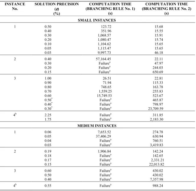
(18) 124. 1. 2. Update current hyperrectangle. Find the left and right dual bounds, store the optimal flows, and find the maximum dual bound. Find the dual bound and store optimal flows. y. 4. Max. dual bound < Best feasible?. Find a new feasible solution*. n. n. Find a new feasible solution*. Dual bound left = Dual bound right? y. n. Select the best of the two feasible solutions. ¿Better than Best_Feasible?. Find the other feasible solution*. y. Update Best_ Feasible. ¿Already ε-optimal?. y. STOP. n. Dual_bd − Fea_sol <ε?. y. 4. n. Store current hyperrectangle. 3. Figure 3. The Global Optimization Procedure (Continued) *. All feasible solutions are found using the successive LP solution procedure shown in Vidal (1998) and Vidal and Goetschalckx (2001).. 4. Computational Experiments The procedure described in the previous section was implemented using AMPL/CPLEX. All the experiments were done in an IBM RS6000 model 590 with 512 MB of RAM. We conducted extensive computational experiments using two sets of instances of different size and all instances were carefully generated to approximate real. instances data. The main characteristics of these instances are shown in Table 1. The procedure was applied to all these instances. Table 2 shows the impact of implementing branching rule No. 2 on the computation time for a set of selected small and medium instances. Clearly, branching rule No. 2 outperforms branching rule No. 1 by dramatically reducing computation times..

(19) 125. Table 1. Main characteristics of the small and medium instances solved CHARACTERISTIC. SMALL INSTANCES. Total number of suppliers Number of internal suppliers Number of manufacturing plants Number of DCs Number of customer zones Number of components Number of finished products Average transportation modes/arc Number of decision variables* Number of constraints* Number of instances in the study *. MEDIUM INSTANCES. 11 3 3 8 20 10 5 2.8 1,544 521 5. 50 12 8 10 80 35 12 3.1 10,100 2,926 5. The number of decision variables and constraints shown correspond to problem PR(x, y, v, z) after preprocessing. Table 2. Impact of branching rule No. 2 on computation time INSTANCE No.. SOLUTION PRECISION (ε ) (%). COMPUTATION TIME (BRANCHING RULE No. 1) (s). COMPUTATION TIME (BRANCHING RULE No. 2) (s). SMALL INSTANCES 1. 0.50 0.40 0.30 0.20 0.10 0.05 0.03. 123.72 351.96 1,068.57 1,080.47 1,104.62 1,115.47 9,997.73. 15.68 15.55 15.91 15.74 15.65 15.65 46.18. 2. 0.40 0.30 0.20 0.15. 57,164.45 Failurea Failurea Failurea. 22.11 47.97 244.03 650.69. 3. 1.00 0.90 0.80 0.70 0.60 0.50* 0.40* 0.30*. 26.51 71.94 748.65 1,559.25 15,749.53 Failurea Failurea Failurea. 22.81 115.33 163.78 255.83 523.67 465.87 798.97 23,709.59. 4b. 2.25 1.75. Failurea Failurea. 311.85 2,183.30. 1. 0.06 0.05 0.04 0.03. 7,653.52 37,406.29 Failurea Failurea. 274.78 630.94 760.51 3,419.83. 2. 0.19 0.18 0.17 0.15. 1,906.84 Failurea Failurea Failurea. 142.24 142.65 2,331.21 22,013.82. 3. 0.60 0.50 0.40. Failurea Failurea Failurea. 430.02 430.02 7,357.98. 4b. 0.55. Failurea. 988.24. MEDIUM INSTANCES. a b. ‘Failure’ means that the process will take more than 100,000 seconds. Instances No. 4 are defined with unconstrained transfer prices (Lower Bound = 0, Upper Bound = A large Number).

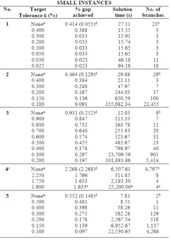
(20) 126. The main results of the implementation of the global optimization procedure are shown in Table 3. The first row of each instance represents the best solution originally found by the successive LP heuristic developed in Vidal (1998) and Vidal and Goetschalckx (2001). Since all upper bounds found by the procedure are global, they can be applied to the solutions given by the primal heuristic algorithm. In this way, a more accurate tolerance can be calculated for each solution given by the successive LP heuristic. This tolerance is shown in parentheses on the first row of each instance, demonstrating that the gaps given by the successive LP primal heuristic were closer to optimality than originally could be established. It is important to note that instances No. 4 were defined with unconstrained transfer prices, that is, with their lower bound equal to zero and their upper bound set to a large number. Thus, instances No. 4 are very unlikely to exist in practice, but they provide a benchmark for the effectiveness and efficiency of the global. optimization procedure. Instances for which the successive LP heuristic finds the optimal solution, are excluded from this table for obvious reasons. Evidently, the global optimization procedure can improve the percentage gap achieved by the successive LP heuristic in reasonable computation time. We also performed some runs to validate the model. Figure 4 shows the response of the model with respect to different increasing values of the market price of a nonprofitable product. When the percentage of increase was initially set to zero, almost 80% of the demand of the product was not satisfied, and the utilization of the two plants that produce the product remained very low. A gradual increase in the market price of the product revealed a significant reduction of the unsatisfied demand and the increase in the utilization of the two plants. Also, the objective function value increased linearly with the increase in market price. This behavior is expected in practice.. Table 3. Performance of the global optimization procedure.

(21) 127. Table 3. (Continued). a. b c. d. e. The successive LP heuristic does not previously specify a target gap; it reaches a local solution that depends on the starting point, and the solution gap can then be calculated by using an upper bound from the relaxed problem. The number of branches corresponds to the number of iterations when referring to the successive LP solution procedure. Instances No. 4 were defined with unconstrained transfer prices, that is, with very large upper bounds. For these instances, the time and number of branches depend on the number of iterations allowed to find each feasible solution since the objective function increase is very slow. The real gap (%) achieved by the successive LP procedure is shown in parentheses, based on the best upper bound found independently by the global optimization procedure. Interrupted after the time shown. If the tolerance improves, then better feasible solutions have been found.. Figure 4. Behavior of unsatisfied demand and percentage of utilization vs. price increase (Medium instance No. 1).

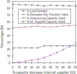
(22) 128. Another experiment was conducted to observe the behavior of the model with respect to transportation mode selection. For the medium instance No. 1, air freight was selected for some of the links when using a holding cost equal to 0.24 $/$.year. When this holding cost was set to zero, the air mode did not appear in the optimal solution, as expected. The objective function value increased by 7.1% in this case. We did a third experiment to analyze the impact of the reduction of the capacity of a key internal supplier. In medium instance No. 1, an internal supplier operates at 100% of utilization, and therefore decreasing its capacity should have a significant impact on the behavior of the system. The capacities of the other internal and external suppliers remained constant in the experiment. Figure 5 shows the behavior of total lost demand, outsourcing, internal sourcing, and the objective function value versus the percentage of decrease in the capacity of this internal supplier. Note that when the capacity of the internal supplier decreases, the overall use of internal suppliers tends to decrease, while outsourcing tends to increase. The objective function value would decrease substantially if the capacity of this supplier were significantly reduced, for instance, in the case of a strike. Finally, note that the lost demand tends to remain approximately constant, as the model looks for the best possible solution.. Figure 5. Behavior of lost demand, outsourcing and internal sourcing vs. percentage capacity decrease of internal suppliers (Medium instance No. 1). The impact of setting transfer prices heuristically and the usefulness of the global optimization procedure were evaluated by the following experiment. First, assume that a company determines the feasible ranges for its transfer prices by taking typical values plus or minus some percentage. This percentage should not exceed 10 percent so that the company can justify its transfer prices to tax authorities. Then, the company sets the transfer prices based on one of the following rules: •. Use the basic transfer prices, that is, the typical values that the company has been using (middle points of the intervals = MID_TP);. •. Use a heuristic rule that sets the transfer price to either its lower or upper bound, if the income tax rate of the origin country is higher (lower) than that of the destination country, respectively (HEU_TP);. •. Use the lower bound for all transfer prices (LB_TP); or. •. Use the upper bound for all transfer prices (UB_TP).. After having set the transfer prices, suppose that the company uses an LP optimization model to determine the optimal flows. The net profit after tax obtained by this process is finally recorded. The company now applies the global optimization procedure presented in this paper, where the feasible ranges for the transfer prices are the same. The results of this contrast are shown in Table 4. The numbers shown in this table represent the profit increase that the company can achieve by using the integrated global supply chain optimization model combined with the global optimization procedure, in comparison to the profit given by the optimal sequential decision process described above. Of course, the company could be operating close to optimality as illustrated in the medium instance No. 1, but having this knowledge is by itself a very important piece of information..

(23) 129. Table 4. Impact of the use of the global optimization procedure on profit maximization. a. Instances No. 4 were not considered in this experiment because they were defined with unconstrained transfer prices.. 5. Conclusions and further research In this paper we describe an integrated global supply chain model that incorporates explicitly transfer prices and transportation cost allocation as decision variables. The resulting problem is a non-convex optimization problem with a linear objective function and a set of bilinear constraints. To solve the problem, we implement the global optimization procedure developed by Ben-Tal et al. (1994). The procedure is most significantly accelerated by reducing the number of dual constraints, by finding tight heuristic upper bounds, by finding good feasible solutions, and by better selecting the branching variables. It has been shown that in this formulation the number of constraints of the dual problem grows polynomially instead of exponentially with respect to the dimension of the vector of the transferprice-related flow variables and therefore the theoretical results in Ben-Tal et al. (1994) could be applied to real-sized instances. The computation times are satisfactory for prescribed gaps within 0.5 percent of the upper bound for real problems. Additionally, the global optimization procedure is useful to show that the optimality gaps found by the primal heuristic presented in Vidal (1998) and Vidal and Goetschalckx (2001) were closer to optimality than originally could be established.. The profits created by the global integrated procedure were compared with the profits of an optimal sequential procedure, where transfer prices are set using a heuristic rule that is common in practice. The results show that MNCs may be able to significantly increase their profit after tax by just determining their transfer prices from known and legal ranges after applying the procedure presented in this paper. The inclusion of discrete location decisions is a fertile area of further research, especially regarding the opening of new DCs in countries where no DC exists, so that the TP decision becomes significant. Additionally, this kind of procedure might be extended to different methods for setting transfer prices, such as fixed markups on variable or total production costs. In these cases, the transfer prices do not have any specific bounds, but can be determined according to the flows and costs found by the optimization model. The authors are investigating such methods and are applying them to the design of global supply chains.. 6. Bibliographical references 1. Abdallah, W.M. (1989). International Transfer Pricing Policies: Decision Making Guidelines for Multinational Companies, Quorum Books, New York..

(24) 130. 2. Abdallah, W.M. (2004). Critical Concerns in Transfer Pricing and Practice, Praeger Publishers, Greenwood Publisher Group, Inc., Westport. 3. Al-Khayyal, F.A. (1990). Jointly constrained bilinear programs and related problems: An overview, Computers & Mathematics with Applications 19(11), 53-62. 4. Al-Khayyal, F.A. (1992). Generalized bilinear programming: Part I. Models, applications and linear programming relaxation, European Journal of Operational Research 60(3), 306314. 5. Al-Khayyal, F.A. & J.E. Falk. (1983). Jointly constrained biconvex programming, Mathematics of Operations Research 8(2), 273286. 6. Al-Khayyal, F.A., C. Larsen & T.V. Voorhis. (1995). A relaxation method for nonconvex quadratically constrained quadratic programs, Journal of Global Optimization 6, 215-230. 7. Androulakis, I.P., C.D. Maranas & C.A. Floudas. (1995). αBB: A global optimization method for general constrained nonconvex problems, Journal of Global Optimization 7, 337-363. 8. Audet, C., J. Brimberg, P. Hansen, S.L. Digabel & N. Mladenovic. (2004). Pooling Problem: Alternate Formulations and Solution Methods. Management Science 50(6), 761-776. 9. Ben-Tal, A., G. Eiger & V. Gershovitz. (1994). Global minimization by reducing the duality gap, Mathematical Programming 63, 193-212. 10. Bloemhof-Ruwaard, J.M. & E.M.T. Hendrix. (1996). Generalized bilinear programming: An application in farm management, European Journal of Operational Research 90(1), 102114. 11. Canel, C. & B.M. Khumawala. (1997). Multiperiod international facilities location: An algorithm and application, International Journal of Production Research 35(7), 1891-1910. 12. Cohen, M.A., M. Fisher & R. Jaikumar. (1989). International manufacturing and distribution networks: A normative model framework, in: K. Ferdows (editor), Managing International Manufacturing, North-Holland, Amsterdam, 6793. 13. Cohen, M.A. & H.L. Lee. (1989). Resource deployment analysis of global manufacturing and distribution networks, Journal of Manufacturing Operations Management 2, 81104. 14. Fandel, G. & M. Stammen (2004). A general model for extended strategic supply chain. 15.. 16.. 17.. 18.. 19.. 20.. 21.. 22.. 23.. 24.. 25.. 26.. management with emphasis on product life cycles including development and recycling. International Journal of Production Economics 89(3), 293-308. Floudas, C.A. & A. Aggarwal. (1990). A decomposition strategy for global optimum search in the pooling problem, ORSA Journal of Computing 2(3), 225-235. Floudas, C.A. & V. Visweswaran. (1990). A global optimization algorithm (GOP) for certain classes of nonconvex NLPs—I. Theory, Computers & Chemical Engineering 14(12), 1397-1417. Floudas, C.A. & V. Visweswaran. (1993). Primal-relaxed dual global optimization approach, Journal of Optimization Theory and Applications 78(2), 187-225. Gallo, G. & A. Ülkücü. (1977). Bilinear programming: An exact algorithm, Mathematical Programming 12, 173-194. Gernon, H. & G.K. Meek. (2000). Accounting: An International Perspective, fifth edition, McGraw-Hill/Irwin, Chicago. Goetschalckx, M., C.J. Vidal & K. Dogan (2002). Modeling and design of global logistics systems: A review of integrated strategic and tactical models and design algorithms. European Journal of Operational Research 143(1), 1-18. Júdice, J.J. & A.M. Faustino. (1991). A computational analysis of LCP methods for bilinear and concave quadratic programming, Computers & Operations Research 18(8), 645654. Killian, S. (2006). Where’s the harm in tax competition? Lessons from US multinationals in Ireland. Critical Perspectives on Accounting 17(8), 1067-1087. Lakhal, S.Y. (2006). An operational profit sharing and transfer pricing model for networkmanufacturing companies. European Journal of Operational Research 175(1), 543-565. Meijboom, B. & B. Obel (2007). Tactical coordination in a multi-location and multi-stage operations structure: A model and a pharmaceutical company case. Omega 35(3), 258-273. Miller, T. & R. de Matta (2008). A Global Supply Chain Profit Maximization and Transfer Pricing Model. Journal of Business Logistics 29(1), 175-199. Nieckels, L. (1976). Transfer Pricing in Multinational Firms: A Heuristic Programming.

(25) 131. 27.. 28.. 29.. 30.. 31.. 32.. 33.. 34.. 35. 36.. Approach and a Case Study, John Wiley & Sons, New York. O’Connor, W. (1997). International transfer pricing, in: Frederick D. S. Choi (editor), International Accounting and Finance Handbook, second edition, John Wiley & Sons, Inc., New York. Pardalos, P.M. & S.A. Vavasis. (1991). Quadratic programming with one negative eigenvalue is NP-hard, Journal of Global Optimization 21, 843-855. Qu, S.-J., Y. Ji & K.-C. Zhang. (2008). A deterministic global optimization algorithm based on a linearizing method for nonconvex quadratically constrained programs. Mathematical and Computer Modelling, Article in Press, doi:10.1016/j.mcm.2008.04.004. Rosenthal, E.C. (2008). A game-theoretic approach to transfer pricing in a vertically integrated supply chain. International Journal of Production Economics 115(2), 542-552. Shen, P., Y. Duan & Y. Ma. (2008). A robust solution approach for nonconvex quadratic programs with additional multiplicative constraints. Applied Mathematics and Computation 201(1-2), 514-526. Sherali, H.D. & C.M. Shetty. (1980). A finitely convergent algorithm for bilinear programming problems using polar cuts and disjunctive face cuts, Mathematical Programming 19, 14-31. Sherali, H.D. & A. Alameddine. (1992). A new reformulation-linearization technique for bilinear programming problems, Journal of Global Optimization 2, 379-410. Sherali, H.D. & C.H. Tuncbilek. (1992). A global optimization algorithm for polynomial programming problems using a reformulationlinearization technique, Journal of Global Optimization 2, 101-112. Stitt, I. (1995). Transfer pricing for the next century, Accountancy 116, 92-94. Tuy, H. (1998). Convex Analysis and Global Optimization (Nonconvex Optimization and its Applications), Kluwer Academic Publishers, Dordrecht, The Netherlands.. 37. Ulstein, N.L., M. Christiansen, R. Gronhaug, N. Magnussen & M.M. Solomon (2006). Elkem Uses Optimization in Redesigning its Supply Chain. Interfaces 36(4), 314-325. 38. Vidal, C.J. (1998). A Global Supply Chain Model With Transfer Pricing and Transportation Cost Allocation, Unpublished Ph.D. Dissertation, School of Industrial and Systems Engineering, Georgia Institute of Technology, Atlanta, GA. 39. Vidal, C.J. & M. Goetschalckx. (2000). Modeling the effect of uncertainties on global logistics systems, Journal of Business Logistics 21(1), 95-120. 40. Vidal, C.J. & M. Goetschalckx. (2001). A global supply chain model with transfer pricing and transportation cost allocation, European Journal of Operational Research 129(1), 134-158. 41. Vila, D., A. Martel & R. Beauregard (2006). Designing logistics networks in divergent process industries: A methodology and its application to the lumber industry. International Journal of Production Economics 102(2), 358378. 42. Villegas, F. & J. Ouenniche (2008). A general unconstrained model for transfer pricing in multinational supply chains. European Journal of Operational Research 187(3), 829-856. 43. Visweswaran, V. & C.A. Floudas. (1990). A global optimization Algorithm (GOP) for certain classes of nonconvex NLPs—II. Application of theory and test problems, Computers & Chemical Engineering 14(12), 1419-1434. 44. Visweswaran, V. & C.A. Floudas. (1993). New properties and computational improvement of the GOP algorithm for problems with quadratic objective functions and constraints, Journal of Global Optimization 3, 439-462. 45. Wilhelm, W., D. Liang, B. Rao, D. Warrier, X. Zhu & S. Bulusu (2005). Design of international assembly systems and their supply chains under NAFTA. Transportation Research Part E 41(6), 467-493..

(26) 132.

(27)