Quantitative spatial analysis of deforestation in legal amazon: selected topics

Texto completo

(1)DOCTORAL THESIS 2016 TOURISM AND ENVIRONMENTAL ECONOMICS QUANTITATIVE SPATIAL ANALYSIS OF DEFORESTATION IN LEGAL AMAZON: SELECTED TOPICS. Tomas Jusys. Thesis Supervisor: prof. William Nilsson Thesis tutor: prof. Catalina Natividad Juaneda Sampol Doctor by the Universitat de les Illes Balears.

(2) © 2016 – Tomas Jusys All rights reserved.

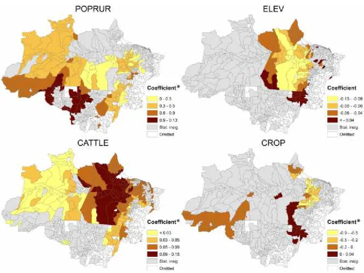
(3) Abstract The dissertation covers five topics on deforestation in Legal Amazon. The first study investigates spatial heterogeneity of deforestation determinants at municipality level. Spatial differences are assessed by geographically weighted regression. The distances between regression points are measured in travel time. The computation is done programmatically. Different drivers of deforestation emerge in different locations of Legal Amazon. For Pará and its surroundings, cattle market is an especially strong driver of deforestation. Crop cultivation leads to forest clearings only in a relatively small area, located in southeastern Pará and northeastern Mato Grosso. Rural credit constraints are effective in curbing deforestation in Pará. Here less deforestation happens where more forests are legally protected, where precipitation levels are favorable for agriculture and at lower altitudes. U-shaped environmental Kuznets curve is concluded for the entire region. However, significant links are found only in Amazonias, Roraima, Pará and its proximities. Timber value motivates deforestation in most parts of the Amazon biome. Official roads contribute to deforestation in Amazonias, Roraima and their surroundings. Adverse effect of unofficial roads on extant forests is especially evident in northern Rondônia and northeastern Pará. Links between rural population and deforestation are very strong for western parts of Rondônia and Mato Grosso, but are very weak in Pará. The implementation of economic distances relative to Euclidean distances changes the results significantly for some regions. The second article investigates whether sugarcane expansion in southern Brazil exports deforestation into the Amazon. This indirect land use change is captured using spatial Durbin model. The parameters are estimated by fixed-effects regression. The results indicate that sugarcane expansion exported 16.3 thousand km2 (12.2%) of deforestation during period 2002-2012, which is equivalent of 189.4 Mg of carbon emissions. The third study contributes to the polemics of whether rural population is linked with deforestation on forest edges. Empirical strategy is as follows: Pará state is partitioned into 5x5 km grids, only cells that classify as forest frontier are retained, links between deforestation and its covariates (including rural population) are investigated both parametrically (fractional logistic regression) and non-parametrically (regression tree). The results confirm positive link between the size of rural communities and deforestation on forest frontiers. Both methods suggest that deforestation is positively linked with cattle herd size and distance to the most proximate river and negatively linked with forest cover and precipitation. Regression tree also reveals that deforestation within protected areas is substantially lower. The fourth paper quantifies avoided deforestation in Pará’s protected areas, on their edges and in their peripheral areas (buffer zones) by matching. Location characteristics are converted into a single propensity score by the means of logistic regression. Pará avoided ~2900 km2 of deforestation during 2000-2004. Space has huge implications: conservation units in remote regions do not avoid deforestation, whereas protected areas near deforestation hotspots save substantial areas of forests. Avoided deforestation is positive in buffer zones located to the west of highway BR-163 and on the banks of Amazon River, and negative in buffers located in eastern Pará. Boundaries of conservation units are well protected from edge effects. The last study maps deforestation at 5x5 km grids in selected territory in Rondônia from past and time-fixed factors. Eigenvector-based spatial filtering is applied to solve spatial autocorrelation problem and to improve mapping accuracy. Output values of trained artificial neural network satisfactory correlate with actual values (correlation coefficient is 0.79).. iii.

(4) Resumen La tesis cubre cinco tópicos distintos sobre la deforestación en Amazonia Legal. El primer estudio investiga la heterogeneidad espacial de determinantes de deforestación a nivel municipal. Las diferencias espaciales son evaluadas por regresión geográficamente ponderada. Las distancias entre puntos de regresión están medidas por tiempo de viaje. Según el estudio, la ganadería afecta a la deforestación más en Pará y sus alrededores. El cultivo de las cosechas aumenta la deforestación sólo en el sureste de Pará y nordeste de Mato Grosso. Las restricciones de crédito rural son una medida eficaz contra la deforestación en Pará. Aquí hay menos deforestación en las zonas con más bosques bajo protección legal, con niveles de precipitación favorables para la agricultura y en alturas más bajas. La relación entre PIB per cápita y deforestación sigue la curva en forma U. El valor de la madera explica la deforestación en la mayoría de las regiones del bioma Amazónico. En general, las carreteras contribuyen a la deforestación más en las regiones remotas. Los vínculos entre población rural y deforestación son más fuertes en el norte de Rondônia y norte de Mato Grosso. La implementación de las distancias por tiempo de viaje con respecto a las distancias Euclidianas cambia los resultados significativamente para algunas regiones. El segundo artículo investiga si la expansión de la caña de azúcar en el sur de Brazil exporta deforestación a la frontera. Los vínculos indirectos entre caña de azúcar y deforestación están capturados por modelo espacial de Durbin. Los parámetros están estimados por regresión de efectos fijos. La caña de azúcar exportó 16.3 miles de km2 (12.2%) de deforestación durante el periodo 2002-2012, el equivalente de 189.4 Mg de las emisiones de carbono. El tercer estudio prueba empíricamente la declaración que la población rural está positivamente relacionada con la deforestación en los bordes del bosque. El estado de Pará se divide en cuadrículas de 5x5 km. Las relaciones entre deforestación y sus determinantes (incluyendo población rural) están investigados por dos métodos: regresión logística fraccional y árbol de regresión. Los resultados confirman que el tamaño de las comunidades rurales está relacionado con la deforestación. Además, ambos métodos sugieren que la deforestación está vinculada positivamente con el tamaño del rebaño bovino y la distancia al río más cercano, y negativamente con la cubierta forestal y la precipitación. El árbol de regresión revela que la deforestación es significativamente más baja dentro de las áreas protegidas. El cuarto artículo cuantifica la deforestación evitada en las áreas protegidas, en sus bordes y en sus zonas parachoques en Pará por método de pareamiento. Las características de localidades están convertidas en un único puntaje de propensión por regresión logística. Pará evitó ~2900 km2 de deforestación durante 2000-2004. El espacio tiene implicaciones importantes: unidades de conservación en las regiones remotas no evitan la deforestación, mientras que áreas protegidas ubicadas cerca de los focos de deforestación salvan grandes áreas de bosques. La deforestación evitada es positiva en las zonas parachoques ubicadas hacia el oeste de la autopista BR-163 y en las orillas del río Amazonas, y negativa en las zonas parachoques situadas en el este de Pará. Los límites de las unidades de conservación están bien protegidos de los efectos de borde. El último estudio simula deforestación en cada cuadrícula de 5x5 km. Mediante filtrado espacial los vectores propios que solucionan el problema de autocorrelación espacial (y automáticamente mejoran la precisión de la predicción) están identificados. Los valores de deforestación están calculados por la red neuronal artificial. El coeficiente de correlación entre los valores reales y los simulados es 0.79).. iv.

(5) Resum La tesi cobreix cinc tòpics distints sobre la deforestació a l’Amazònia Legal. El primer estudi investiga la heterogeneïtat espacial de determinants de deforestació a nivell municipal. Les diferències espacials són avaluades per regressió geogràficament ponderada. Les distàncies entre punts de regressió estan mesurades per temps de viatge. Segons l’estudi, la ramaderia afecta la deforestació més a Pará i els seus voltants. El cultiu de les collites augmenta la deforestació només a la zona ubicada al sud-est de Pará i nord-est de Mato Grosso. Les restriccions de crèdit rural són una mesura eficaç contra la deforestació a Pará. Aquí hi ha menys deforestació a les zones amb més boscos amb protecció legal, amb nivells de precipitació favorables per a l’agricultura i a altures més baixes. La relació entre PIB per càpita i deforestació segueix la curva en forma d’U. El valor de la fusta explica la deforestació a la majoria de les regions del bioma Amazònic. En general, les carreteres contribueixen a la deforestació més a les regions remotes. Els vincles entre població rural i deforestació són més forts en el nord de Rondônia i nord de Mato Grosso. La implementació de les distàncies per temps de viatge respecte de les distàncies Euclidianes canvia els resultats significativament per a algunes regions. El segon article investiga si l’expansió de la canya de sucre a les regions d’Amazònia Legal fora del bioma Amazònic exporta deforestació al bioma. Els vincles distants entre canya de sucre i deforestació estan capturats per model espacial de Durbin. Els paràmetres estan estimats per regressió d’efectes fixos. La canya de sucre exportà 16.3 milers km2 (12.2%) de deforestació durant el període 2002-2012. El tercer estudi prova empíricament la declaració que la població rural està positivament relacionada amb la deforestació a les voreres del bosc. L’estat de Pará se divideix en quadrícules de 5x5 km. Les relacions entre deforestació i els seus determinants (incloent població rural) estan investigats per dos mètodes: regressió logística fraccional i arbre de regressió. Els resultats confirmen que la mida de les comunitats rurals està relacionada amb la deforestació. A més, ambdós mètodes suggereixen que la deforestació està vinculada positivamente amb la mida del ramat boví i la distància al riu més pròxim, i negativament amb la coberta forestal i la precipitació. L’arbre de regressió revela que la deforestació és significativament més baixa dins les àrees protegides. El quart article quantifica la deforestació evitada a les àrees protegides, en els seus límits i a les seves zones para-xocs a Pará pel mètode d’aparellament. Les característiques de localitats estan convertides en una única puntuació de propensió per regressió logística. Pará evità ~2900 km2 de deforestació durant 2000-2004. L’espai té implicacions importants: unitats de conservació a les regions remotes no eviten la deforestació, mentre que àrees protegides ubicades a prop dels focus de deforestació salven grans àrees de boscos. La deforestació evitada és positiva a les zones para-xocs ubicades cap a l’oest de l’autopista BR-163 i a les voreres del riu Amazonas, i negativa a les zones para-xocs situades a l’est de Pará. Els límits de les unitats de conservació estan ben protegits dels efectes de límit. El darrer estudi simula deforestació a cada quadrícula de 5x5 km. Mitjançant filtrat espacial els vectors propis que solucionen el problema d’auto correlació espacial (i automáticament milloren la precisió de la predicció) estan identificats. Els valores de deforestació estan calculats per la xarxa neuronal artificial. El coeficiente de correlació entre els valors reals i els simulats és de 0.79).. v.

(6) Table of contents LIST OF FIGURES .........................................................................................................IX LIST OF TABLES ...........................................................................................................XI ACKNOWLEDGEMENTS ..........................................................................................XII Chapter 1. INTRODUCTION ........................................................................................1 1.1. References..................................................................................................................................... 9. Chapter 2. FUNDAMENTAL CAUSES AND SPATIAL HETEROGENEITY OF DEFORESTATION IN LEGAL AMAZON................................................................11 2.1. Introduction ............................................................................................................................... 12 2.2. Data and methods ..................................................................................................................... 13 2.3. Results......................................................................................................................................... 16 2.4. Discussion .................................................................................................................................. 23 2.5. Conclusions................................................................................................................................ 27 2.6. References................................................................................................................................... 27. Chapter 3. A CONFIRMATION OF THE INDIRECT IMPACT OF SUGARCANE ON DEFORESTATION IN THE AMAZON ..................................33 3.1. Introduction ............................................................................................................................... 34 3.2. Research context........................................................................................................................ 35 3.3. Data and methods ..................................................................................................................... 36 3.4. Results and discussion ............................................................................................................. 40 3.5. Conclusions................................................................................................................................ 42 3.6. References................................................................................................................................... 43. Chapter 4. ASSOCIATIONS BETWEEN DEFORESTATION AND POPULATION ON FOREST FRONTIERS IN PARÁ: EMPIRICAL STUDY.......47 4.1. Introduction ............................................................................................................................... 48 4.2. Materials and methods............................................................................................................. 50 4.3. Results......................................................................................................................................... 53 4.4. Discussion and conclusions..................................................................................................... 56 4.5. References................................................................................................................................... 57. Chapter 5. QUANTIFYING AVOIDED DEFORESTATION IN PARÁ: PROTECTED AREAS, BUFFER ZONES AND EDGE EFFECTS ...........................61 5.1. Introduction ............................................................................................................................... 62 vi.

(7) 5.2. Materials and methods............................................................................................................. 64 5.3. Results and discussion ............................................................................................................. 69 5.4. Conclusions................................................................................................................................ 76 5.5. References................................................................................................................................... 77. Chapter 6. USING ARTIFICIAL NEURAL NETWORKS AND EIGENVECTORS TO PREDICT DEFORESTATION AT 5X5 KILOMETER GRIDS...........................79 6.1. Introduction ............................................................................................................................... 80 6.2. Study area................................................................................................................................... 81 6.3. Materials and methods............................................................................................................. 82 6.3.1. Data sources and processing............................................................................................................................83 6.3.2. Covariate selection and spatial filtering.........................................................................................................84 6.3.3. Network calibration ..........................................................................................................................................85. 6.4. Results......................................................................................................................................... 87 6.5. Conclusions................................................................................................................................ 90 6.6. References................................................................................................................................... 90. Chapter 7. CONCLUSIONS.........................................................................................95 7.1. References................................................................................................................................. 101. Chapter 8. APPENDICES ...........................................................................................103 8.1. Appendix A.............................................................................................................................. 104 8.2. Appendix B .............................................................................................................................. 105 8.3. Appendix C .............................................................................................................................. 106 8.4. Appendix D.............................................................................................................................. 107 8.5. Appendix E .............................................................................................................................. 108 8.6. Appendix F .............................................................................................................................. 109 8.7. Appendix G.............................................................................................................................. 110 8.8. Appendix H ............................................................................................................................. 111 8.9. Appendix I ............................................................................................................................... 112 8.10. Appendix J ............................................................................................................................. 113 8.11. Appendix K............................................................................................................................ 114 8.12. Appendix L ............................................................................................................................ 115 8.13. Appendix M ........................................................................................................................... 116 8.14. Appendix N ........................................................................................................................... 117 8.15. Appendix O............................................................................................................................ 118 8.16. Appendix P ............................................................................................................................ 119 8.17. Appendix Q............................................................................................................................ 120 8.18. Appendix R ............................................................................................................................ 121 vii.

(8) 8.19. Appendix S............................................................................................................................. 122. Chapter 9. SUPPLEMENTARY MATERIAL...........................................................123 9.1. GWR-2SLS codes..................................................................................................................... 124 9.2. Fixed-effects code with computation of ILUC variables ................................................... 131 9.3. Spatial filtering codes ............................................................................................................. 136. viii.

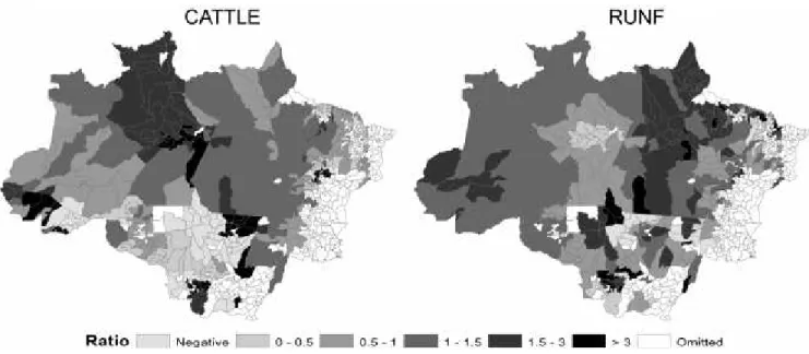
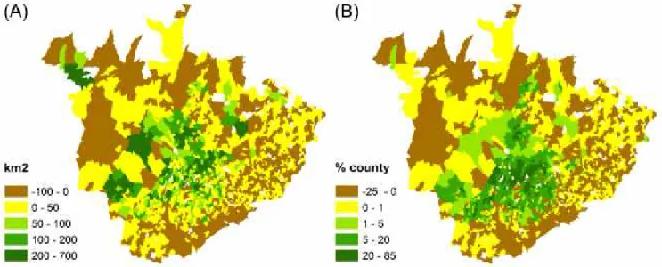
(9) List of figures Figure 1. Spatial distribution of local coefficients of selected variables....................................... 20 Figure 2. Comparison of GWR beta estimates under straight line and travel time distances for cattle ranching (left) and unofficial road network (right) .............................................................. 22 Figure 3. Changes in planted sugarcane area between 2002 and 2012 in agricultural counties (see Figure G1) in terms of square kilometers (left) and percent of county’s territory (right) . 35 Figure 4. Overall mean squared error for various bandwidths (left) and weighting mechanism with optimal bandwith, by road distance (right) ............................................................................ 40 Figure 5. Spatial distribution of deforestation and population on forest frontiers in Pará during 2010-2014 .................................................................................................................................. 54 Figure 6. Pruned regression tree ........................................................................................................ 56 Figure 7. Layers of park protection ................................................................................................... 64 Figure 8. Mean absolute standardized percentage biases (A) and statistical significance of avoided deforestation (B).................................................................................................................... 72 Figure 9. Avoided deforestation in percentages during 2000-2004 year period......................... 73 Figure 10. Parakanã and Mãe Maria (picture taken on 2014 04 30) .............................................. 76 Figure 11. Geographical location of the study area......................................................................... 81 Figure 12. Location of roads, rivers, city of Buritis and conservation units ................................ 82 Figure 13. Covariate selection ............................................................................................................ 84 Figure 14. Graphical illustration of artificial neural network with c inputs and 4 hidden neurons .................................................................................................................................................. 85 Figure 15. Spatial distribution of OLS (A) and OLS-E (B) residuals............................................. 87 Figure 16. Actual and simulated deforestation in 2014 .................................................................. 88 Figure 17. Matching and commission rates for different thresholds............................................ 89 Figure A1. Road and river network in Legal Amazon.. ............................................................... 104 Figure E1. Local determination coefficients. .................................................................................. 108 Figure F1. Territorial changes of Brazilian counties between 2000 and 2014 ........................... 109 Figure G1. Deforestation and agricultural counties with road connection. .............................. 110 Figure H1. Total weighted indirect effect (the sum of current and lagged weighted indirect effects) of sugarcane measured in hectares during 2002-2012..................................................... 111 Figure J1. Population data (WorldPop) accuracy assessment ..................................................... 113 Figure L1. Map of Pará ...................................................................................................................... 115 ix.

(10) Figure O1. Spatial patterns of characteristics................................................................................. 118 Figure P1. Protected areas in Pará by characteristics (year of establishment, type of governance, and IUCN category) .................................................................................................... 119 Figure Q1. Contagious deforestation .............................................................................................. 120 Figure S1. Map patterns of the first six eigenvectors .................................................................... 122. x.

(11) List of tables Table 1. Description of the variables (chapter 2) ............................................................................. 14 Table 2. Spatial autocorrelation and Moran’s I ................................................................................ 17 Table 3. Results of global regressions................................................................................................ 17 Table 4. Variability of local coefficients ............................................................................................ 19 Table 5. Description of the variables (chapter 3) ............................................................................. 37 Table 6. Regression results (chapter 3).............................................................................................. 41 Table 7. Regression results (chapter 4).............................................................................................. 55 Table 8. Determinants of propensity score....................................................................................... 69 Table 9. Balance statistics: mean absolute standardized percentage bias (MASPB) after matching and percentage of bias elimination (BE) ......................................................................... 70 Table 10. Average treatment effects on the treated by park characteristics ................................ 71 Table 11. Edge effect analysis ............................................................................................................. 74 Table 12. Moran’s I of model residuals ............................................................................................. 87 Table 13. Prediction power of OLS and OLS-E models.................................................................. 88 Table B1. Descriptive statistics for municipalities......................................................................... 105 Table C1. Correlation matrix for municipalities ............................................................................ 106 Table I1. Collinearity statistics ......................................................................................................... 112 Table K1. Descriptive statistics (grid level) .................................................................................... 114 Table M1. Marginal effects of variables .......................................................................................... 116 Table N1. Regression tree: detailed statistics ................................................................................. 117 Table R1. Multicollinearity statistics: variance inflation factors (VIFs), condition numbers, and determinants of correlation matrices .............................................................................................. 121. xi.

(12) Acknowledgements I would like to express my sincere gratitude to the University of the Balearic Islands for financial support that lasted 4 years. I greatly thank my supervisor prof. William Nilsson for continuous support and detailed comments and suggestions toward improving every manuscript, especially in the field of econometrics. I also thank William for organizing internal seminars, which gave me the opportunity to present my work to ampler audiences and receive feedback from other professors. Additionally, I give credit for prof. Andreu Sansó Roselló for detailed review of chapter 2, prof. José Luis Groizard for detailed review of chapter 5, prof. Tomás del Barrio Castro and Andrii Bodnar for useful overall comments. Finally, I thank my fellow Ernestas Zabarauskas for writing a computer script that collects Google distances and Stefânia Costa from IMAZON for providing the shapefile of Amazon’s unofficial roads. All remaining errors and omissions are my own.. xii.

(13) Chapter 1 Introduction. 1.

(14) Massive rainforest deforestation takes place in a limited number of countries. Nonetheless, the consequences are global. Large amount of carbon stock is released into the atmosphere. Thus, forest clearings fuel the process of global warming, which is a widely discussed topic in today’s political summits. Besides, continuous deforestation threatens a variety of endemic species and nature’s genetic resources in general. Some reasons leading to deforestation are also global. Deforestation is often fueled by commercial agriculture, and the scope of agriculture is defined by the global demand of agricultural commodities. Global implications of deforestation underlie its importance and promote interest into the topic. Brazil faces the largest annual deforestation in terms of total area cleared among all countries. Deforestation in Brazil came with colonization. By the end of the 19th century, most of the Atlantic forests in Brazil’s northeast, south and center-south were cut. Agriculture was primarily responsible for further clearings in center-western and northern regions during the second half of the 20th century (Araujo et al., 2011). Early governments of Brazil favored colonization into the Brazilian Amazon. It wasn’t until the eighth decade of the 20th century that deforestation raised serious concerns for governmental institutions. However, massive deforestation continued to soar, reaching its peak in 2004. Since then, combined efforts of the Brazilian government and NGOs coupled with global economic crisis led to a significant reduction in deforestation rates. Despite this, current level of forest loss remains a huge treat to environmental sustainability. Deforestation is a complex phenomenon. It is influenced, among other factors, by economic activities, infrastructure layout, demographics, terrain characteristics and legal enforcement. The connections between deforestation and its determinants sometimes are bidirectional and often manifest indirectly through other phenomena. Occasionally, deforestation is affected by distal factors. Most importantly, causes of deforestation cannot be generalized to all locations. As a consequence, policy measures to mitigate deforestation can be effective only if local contexts are properly addressed. Spatial heterogeneity of the processes that affect deforestation remains incomprehensively researched. Therefore, the main objective of this dissertation is to empirically investigate the interactions between deforestation and various factors by addressing spatial differences. This dissertation is comprised of five self-contained studies. The first study investigates direct and underlying causes of deforestation and how those factors affect deforestation in different locations across Legal Amazon. The second work answers the question whether sugarcane expansion in southern Brazil exports deforestation into the Amazon. The third investigation empirically tests the theory that rural communities are responsible for deforestation on forest frontiers. The fourth paper builds on researches into the influence of legal forest protection on deforestation by measuring avoided deforestation in conservation units, in buffer zones, and on the edges of conservation units. The last study aims to map deforestation from past and time-fixed variables by exploiting spatiotemporal contagion of deforestation. Causes of deforestation, both direct and underlying, are widely analyzed in academic literature. Key direct causes of deforestation in Legal Amazon, as indicated by most investigators, are agriculture and infrastructure. Agriculture consists of livestock (mostly cattle) and crop 2.

(15) cultivation (mostly soybean and sugarcane) businesses. Agriculture in Brazil relies heavily on the credit system. The official rural credit portfolio covers about a third of the annual financial needs of the agricultural sector in Brazil (Assunção et al., 2013b). Rural credit is loaned in accordance to rules and conditions issued by the Central Bank of Brazil. However, this money in the hands of farmers may fuel deforestation. In response to such fears, in 2008 Resolution 3545 was released, which conditioned the concession of rural credit for use in agricultural activities in the Amazon Biome upon presentation of proof of borrowers’ compliance with environmental legislation, as well as of the legitimacy of their land claims and the regularity of their rural establishments. Among documents needed was the declaration stating the absence of current embargoes caused by economic use of illegally deforested areas (Assunção et al., 2013b). However, rural credit concessions do not necessarily increase deforestation. As Assunção et al. (2013b) notice, crop farmers are likely to invest a larger share of rural credit loans in the intensification of production, instead of expanding it by operating in the extensive margin as cattle ranchers do. Indeed, there are important differences between cattle ranching and crop cultivation in terms of pressure on forests. Geo-ecological barriers are in general more restrictive in the case of crop cultivation (Margulis, 2004), making cattle ranching the predominant industry. Numerically, ranching enterprises occupy roughly 75 percent of the deforested areas of Legal Amazon. The key restriction for plant cultivation is high rainfall (the other important constraint is steep slope), causing most problems during seeding and harvesting. Topographic and climatic characteristics vary across Legal Amazon, and, as a result, land suitability for crop cultivation. This is a strong argument in favor of models that capture spatial heterogeneity. Another widely recognized determinant of deforestation is road network. A classic example of road-induced deforestation is the Trans-Amazonian highway, opened in the eighth decade of previous century. Thus, not constructing a road is a way to prevent deforestation. However, even bigger concern is the network of unofficial roads. These roads are generally built to open up forests to illegal logging, thus leading to new colonization, forest fragmentation, ecological degradation and increased fire risk (Barber et al., 2014). Market growth and foreign trade are often named as contributors to deforestation. Both crop cultivation and cattle ranching satisfy both national and international markets. International demand of Brazilian products increases the need to deforest. Some efforts to mitigate international pressure on Brazilian rainforests have been made. For example, under the pressure of retailers and NGOs, major soybean traders signed Brazil’s Soy Moratorium, which is a voluntary agreement not to purchase soy grown on lands, deforested after July of 2006. However, weaknesses in federal enforcement aggravate the potential of this initiative. Currently, for more than half of registered properties with embargoes producer identification is inconsistent with the system of Rural Environmental Registry of private properties (Gibbs et al., 2015b). This system is used by soy traders to check for embargoes. Since information is inconsistent, transactions with properties under embargoes continue to happen. Similarly, meatpacking companies in Pará began signing the legally binding Terms of Adjustment of Conduct (known as TAC), committing to purchase cattle only from ranchers registered with the Pará State Rural Environmental Register. Furthermore, in 2009 Brazil’s largest slaughterhouses (JBS-Bertín, Marfrig and Minerva) signed an agreement with Greenpeace not to purchase 3.

(16) meat production from ranches with deforestation (Gibbs et al., 2015a). The initiative only considers direct suppliers, thereby leaving plenty of room to circumvent commercialization restrictions. Trade of agricultural products, especially beef, continues to soar. The biggest importers of Brazilian beef are Russia, Hong Kong, Venezuela and Egypt (SECEX-MDIC, 2015). Arguably, ever increasing demand of agricultural products is a consequence of growing populations in foreign trade partners, because larger populations imply higher meat consumption. Naturally, the size of population emerges as a potential direct cause of deforestation. Here the distinction is often made between rural and urban communities. Indeed, there is an ongoing debate among scholars, whether rural or urban population contributes to deforestation to a higher extent. Authors, who argue that urban population growth rather than rural population growth is a stronger accelerant of deforestation, defend their position by arguing that urbanization raises consumption levels and increases demand for agricultural products. DeFries et al. (2010) claim that urban consumers generally eat more processed foods and animal products than rural consumers, thereby stimulating commercial production of crops and livestock. On the contrary, Wright & Muller-Landau (2006) find that recent deforestation rates are positively related to local rural population density, and that the percent of the remaining forests is often negatively related to rural population density in the tropics. Key arguments in favor of rural-driven deforestation are immigration and high natality rate (Izquierdo et al., 2011). The relationships between deforestation and its determinants are region-specific (Margulis, 2004), but most academic studies ignore this fact. To the best knowledge of the author, only Oliveira & Almeida (2011) investigated the causes of deforestation from local perspective in Legal Amazon at county level. This was achieved by applying geographically weighed regression (GWR). However, these authors were restricted to the limited capabilities of the software that estimates GWR, which led them to make two very restrictive assumptions. Specifically, those assumptions are: 1) all covariates are strictly exogenous, and 2) Euclidean distances reflect well the communications between municipalities. As already discussed, deforestation is potentially explained by the size of populations. However, as Angelsen & Kaimowitz (1999) notice, growing populations affect labor market, technological progress and institutional changes. Thus, deforestation itself may attract new inhabitants as a result of these changes. Similar argument applies to national income. However, its effect on deforestation can be both positive and negative. Higher national income creates additional job opportunities outside agricultural sector, thus reducing pressure on forests, but higher income also increases the production of agricultural and timber products, thus stimulating deforestation. Furthermore, deforestation itself is a source of income. Therefore, both population and national income shall be treated as endogenous in deforestation modeling. The application of GWR method requires distances between the regression points (municipality seats in this dissertation). Euclidean distances, most often used by the researchers, may not be a proper representation of communications inside Legal Amazon. Most logged woods are transported by roads in trucks. However, these roads in Legal Amazon often are winding due to geographical constraints, financial gains in building a single road that stretches through multiple towns, or unwillingness to pave a road that crosses intact forests to avoid potential 4.

(17) deforestation. Moreover, roads are not homogenous in quality: some roads are highways and some are not paved. This has important implications on travel time. Furthermore, Legal Amazon hosts around 100 towns that do not have access by roads. These towns are located on the banks of the Amazon River or other major river in Legal Amazon. Connections between these towns are based on water transport. Rivers, especially smaller, meander to a high extent, thus extending the distance and time required to travel to a destination. Chapter 2 investigates the main causes of deforestation in Legal Amazon. The findings of the linear model under endogenous treatment of population and GDP per capita are presented. Further, GWR based on economic (travel time) distances is applied to assess spatial heterogeneity of deforestation determinants. This is done programmatically. The code is written in Gauss platform, and is author’s own elaboration. Also, a comparative analysis on how the implementation of economic distances instead of straight line distances changes the results is presented. Complete analysis of deforestation determinants must consider the possibility that cause and effect are separated in space. It is widely theorized that in Brazil crop planters displace cattle ranchers into the Amazon, thereby indirectly contributing to deforestation. The displacement happens because the farmers residing in non-frontier regions sell their pastures to crop businesses and move to the frontier, where they purchase land from local smallholders. This phenomenon is known as indirect land use change (ILUC). To understand the reasons of ILUC, it is necessary to discuss the economic and geo-climatic context of Brazil. The territory of Brazil can be partitioned into two major zones that differ in conditions for agriculture. For simplicity I refer to those as agricultural and frontier zones. The former are located outside the Amazonian Biome and are characterized by high land prices and unavailability of productive land (especially, in closer proximities to the frontier). In most parts both crop cultivation and livestock farming can be practiced due to favorable climatic and topographic conditions. Conversely, the frontier is covered by vast areas of available and inexpensive land (forests to be cleared). However, due to high level of rainfall, crops cannot be readily cultivated. In economic terms this means that the frontier has a comparative advantage for livestock farming as opposed to crop cultivation. An economic factor that encourages farmers to sell land properties to crop planters in agricultural zones and move to the frontier is high differential in land prices (Sawyer, 2008). Various crops are cultivated in Brazil, but the most widespread are soybean and sugarcane. Sugarcane is the main source of ethanol biofuel. Ethanol is widely used in Brazil in the transport industry. Its production is likely to expand further due to the potential size of the domestic market and to the opportunities for exporting (Walter et al., 2014). Due to the fact that growing sugarcane absorbs more carbon than is emitted when the ethanol is burned as fuel, ethanol is considered as a potential solution to global warming problem. The later statement relies on the assumption that sugarcane has no influence on deforestation. Empirical findings from the Amazon region generally show that sugarcane and deforestation are not directly linked. However, in case sugarcane planters displace livestock farmers into the Amazon, and, as a result, export deforestation, the superiority of ethanol over fossil fuel in terms of reducing CO2 emissions may be overstated. 5.

(18) Much of the academic literature focuses on ILUC associated with soybean, the primary crop in Brazil. Several studies indirectly linked soybean with deforestation in the Amazon. However, empirical evidence of ILUC associated with sugarcane is scant. Therefore, chapter 3 empirically tests the hypothesis that sugarcane planters in southern Brazil contribute to deforestation in the Amazon Biome, and measures the magnitude of the effect. The study uses 20022012 panel dataset. Indirect linkages between sugarcane expansion in southern Brazil and deforestation are captured using spatial Durbin model. The parameters are estimated by fixedeffects regression. Large producers who move to the frontier purchase lands from smaller producers. Questions, such as where those small producers come from and whether they contribute significantly to deforestation have to be answered. Rural family children in Legal Amazon follow one of the three alternatives in terms of migration. Some move to urban areas to seek off-farm employment, which enables to diversify risks and overcome credit constraints. Some new generation rural inhabitants remain on the farm. Finally, some move to forest edges. Even though those are relatively few, Carr & Burgdorfer (2013) theorize that rural farmers residing near forest edges have a disproportionally large adverse effect on extant forests, since newly arrived rural migrants often engage in expansive agriculture due to cheap family labor, scarce capital, low technology, high cost of transportation and insecure land tenure. The latter implies that as soon as new migrants arrive, they establish their farming systems and cut down trees to demonstrate land claims (Simmons et al., 2003). Later, these farmers seek official recognition of the land which they developed. As more rural migrants arrive, land availability decreases. As it happens, some farmers move to another undisturbed location on forest edge. Their previously developed lands are sold for large scale producers. Those lands are then consolidated to create large enough areas for cattle grazing or cultivation of commercial crops. The relationship between deforestation and rural population may be different on forest frontiers and in long-settled rural areas. Long-settled rural areas are covered by large pastures or crop fields. The consumer of agricultural commodities that originate from those areas is often a foreign citizen. Therefore, distal demands of agricultural production is what control land use change in old rural settlements. This, in turn, implies that local rural population here is not a significant component of deforestation function or at least drives forest clearings to a lesser extent than on forest edges. Forest edges are characterized by abundant and undisturbed forest resources. As discussed, here migrant rural settlers engage in extensive deforestation, thereby opening large previously inaccessible areas for colonization. An additional rural migrant here creates a lot of pressure on standing forests. As a result, a separate analysis is needed to understand the associations between deforestation and rural demographics on forest edges. Chapter 4 presents such a study, which empirically tests the argument of Carr & Burgdorfer (2013) that rural settlements are linked with deforestation on forest edges. Selected study area encompasses the state of Pará. To properly capture the associations between deforestation and its covariates on forest edges fine scale analysis is needed. Therefore, the territory of Pará is partitioned into 5x5 km grids. Besides rural population, all relevant and available covariates are included. The analysis is based both on parametric (fractional logistic regression) and 6.

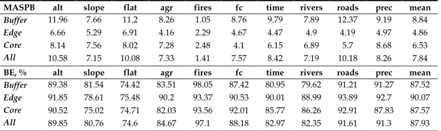
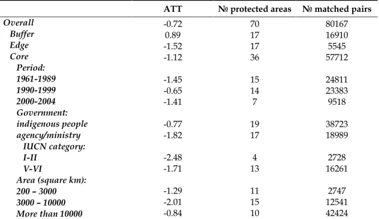
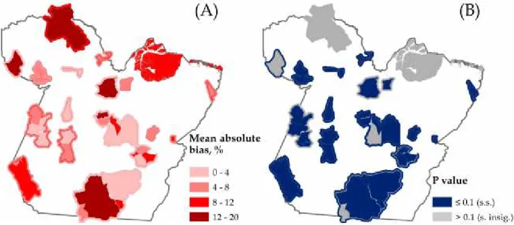
(19) non-parametric (regression tree) approaches. The findings also complement the analysis in chapter 2, as the links between deforestation and its explanatory factors in some instances may be scale-dependent (Pan & Carr, 2010). As discussed, land insecurity in Brazil creates incentives to deforest (Araujo et al., 2011) and is a consequence of weaknesses in legislation. The Land Statute of Brazil states that squattersI who are developing a land during at least five consecutive years and are not in a conflict with landowners can claim formal property title over that land. Moreover, the Brazilian Constitution of 1988 states that unproductive establishments can be taken over and redistributed to other parties. Such legislation creates incentives to clear forests, since forests are considered as unused lands. One of key measures in combating land insecurity in Brazil is the protected area system. The legal framework of the system was established in 2000 by the National Protected Areas System Law (SNUC). In 1998 the Amazon Region Protected Areas Program (ARPA) was formulated. The program foresaw the establishment of 15 conservation units under strict protection during four-year period (between 2000 and 2003). Later, in 2005 and 2006, the network of protected areas in Legal Amazon was expanded drastically, especially in the state of Pará. However, protected area itself is only a part of protection mechanism. Conservation units are surrounded by buffer zones. A buffer zone is a peripheral area around a conservation unit and is meant to benefit local populations by allowing low environmental impact activities. In this way it is expected that local inhabitants will be involved in the protection of a conservation unit near their residence. However, the establishment of protected areas may provoke displacement of deforestation locations (substitution effect). It is probable that loggers move to the surroundings of a newly created conservation unit instead of entering the protected territory, which they would have entered if that territory had remained unprotected. Therefore, avoided deforestation in buffer zones can be both positive and negative depending on whether effective buffer zone management or substitution effect dominates. Buffer zones also shed protected areas from edge effects. An edge effect in this dissertation is described as an excessive deforestation of park’s edge relative to its internal area. There are at least two reasons why an edge of a conservation unit is subjected to higher deforestation risk: 1) it borders unprotected areas or, even worse, open areas without vegetation, and 2) deforested fields in nearby areas of a conservation unit are dry and can easily catch fire, affecting forests on the edge of a conservation unit. Therefore, buffer zones constitute a shield from those risks. Furthermore, buffer zone management has important implications in ecology, since buffer zones and ecological corridors ensure that species have sufficient habitat to survive and that those species can migrate through the forests. The importance of buffer zones is well understood by the Brazilian government. The Government of Brazil together with the Pilot Program for the Brazilian Rainforests allocated almost 23 million US dollars for buffer zone management under the four-year ARPA project. However, despite the immense importance of buffer zones, their implications on avoided deforestation did not receive sufficient attention from scientists. A meticulous study on avoided deforestation in conservation units of Legal Amazon is found in Nolte et al. (2013), but the study did not consider buffer zones. I. Squatters are individuals who invade lands and develop them, but hold no property rights over those lands.. 7.

(20) To fill the gap of knowledge, chapter 5 investigates the implications of buffer zone management on avoided deforestation in Pará. The percentages of avoided deforestation are estimated by propensity score matching. Edge effects are tested by comparing avoided deforestation on park’s edge and in its nuclear area (park’s territory beyond its edge). Most importantly, buffer zones around protected areas are considered separately for each protected area or a group of protected areas that share borders. Location matters primarily due to the differences in deforestation pressure: some conservation units are located on deforestation frontiers and some are located in remote areas, where forest protection has only a cartographic meaning. Knowing the factors responsible for deforestation and applying measures to counteract it is necessary, but does not suffice. Deforestation monitoring and prediction is equally important. Until 2004 the Brazilian Institute of Environment and Renewable Natural Resources (IBAMA) relied on voluntary reports of logging events. As a result, IBAMA could not locate deforestation at its roots. Finally, in 2004 a near real-time system of deforestation detection (DETER) was introduced. DETER is a satellite-based system that captures and processes georeferenced imagery on forest cover in 15-day intervals (Assunção et al., 2013a). The system uses LANDSAT imagery and is capable of detecting deforested areas that are larger than 25 hectares. Newer images are compared with older images to identify changes in forest cover. The imagery is prepared in a form of georeferenced digital maps. Deforestation identified by those maps is verified by field inspections. Some campaigns to prevent deforestation are initiated by NGOs. For example, Greenpeace uses an airplane to locate illegal log rafts and reports observed rafts to the authorities. In addition, Greenpeace developed a technique based on ultraviolet paint to track illegally chopped woods back to exporting companies. Deforestation monitoring helps to detect deforestation in its initial stage and prevent forests from further exploitation. Chapter 6 offers a detailed methodology to map deforestation from past and time-fixed processes. Mapping is done at 5x5 km grids. To achieve successful results, several aspects have to be taken into consideration. Firstly, deforestation is spatially and temporarily contagious. Spatial contagion implies that deforestation in the neighboring locations increases the probability of deforestation in the reference location. Temporal contagion implies that deforestation that happened in recent past is likely to continue into the future. To account for this spatiotemporal contagion, a deforestation function includes past deforestation and its focal variables. However, contagion creates an econometrical problem known as spatial autocorrelation. Under the presence of spatial autocorrelation, linear model errors include both white noise and unobserved covariates. Filtering those important covariates from the errors of the initial model could greatly improve mapping accuracy. Several methods to accomplish this task have been developed, but the most modern and the most promising technique is eigenvector-based spatial filtering. Eigenvectors represent spatial patterns of different spatial autocorrelation levels. Therefore, filtered eigenvectors are artificial constructs of unobserved covariates and are simply added to the list of explanatory variables. To refine mapping accuracy, variables that control for legal protection, terrain and climatic characteristics, and infrastructure are also included. Deforestation values in chapter 6 are simulated using an artificial neural network. The method captures nonlinearities between deforestation and its determinants and, as a result, provides more precise estimates. 8.

(21) The main findings of this dissertation are synthesized and policy recommendations are given in chapter 7. Chapter 8 includes appendices. Chapter 9 presents programming codes.. 1.1. References Angelsen, A., & Kaimowitz, D. (1999). Rethinking the Causes of Deforestation: Lessons from Economic Models. The World Bank Research Observer, 14(1), 73–98. Araujo, C.E., Araujo Bonjean, C., Combes, J.L., Combes, P.M., & Reis, E.J. (2010). Does Land Tenure Insecurity Drive Deforestation in the Brazilian Amazon? Etudes et Documents. Clermont-Ferrand, France: CERDI. Assunção, J., Gandour, C., & Rocha, R. (2013a). DETERring Deforestation in the Brazilian Amazon: Environmental Monitoring and Law Enforcement. Climate policy initiative. Rio de Janeiro, Brazil: Climate Policy Institute. Assunção, J., Gandour, C., Rocha, R., & Rocha, R. (2013b). Does Credit Affect Deforestation? Evidence from a Rural Credit Policy in the Brazilian Amazon. Climate policy initiative. Rio de Janeiro, Brazil: Climate Policy Institute. Barber, C.P., Cochrane, M.A., Souza Jr., C.M., & Laurance, W.F. (2014). Roads, deforestation, and the mitigating effect of protected areas in the Amazon. Biological Conservation, 177, 203-209. Carr, D., & Burgdorfer, J. (2013). Deforestation Drivers: Population, Migration, and Tropical Land Use. Environment, 55(1). DeFries, R.S., Rudel, T., Uriarte, M., & Hansen, M. (2010). Deforestation driven by urban population growth and agricultural trade in the twenty-first century. Nature Geoscience, 3, 178-181. Gibbs, H.K., Munger, J., L'Roe, J., Barreto, P., Pereira, R., Christie, M., … & Walker, N.F. (2015a). Did Ranchers and Slaughterhouses Respond to Zero-Deforestation Agreements in the Brazilian Amazon? Conservation letters. doi: 10.1111/conl.12175 Gibbs, H.K., Rausch, L., Munger, J., Schelly, I., Morton, D.C., Noojipady, P., … & Walker, N.F. (2015b). Brazil‘s Soy Moratorium. Supply-chain governance is needed to avoid deforestation. Science, 374, 377378. Izquierdo, A.E., Grau, H.R., & Aide, T.M. (2011). Implications of Rural–Urban Migration for Conservation of the Atlantic Forest and Urban Growth in Misiones, Argentina (1970–2030). Journal of Human Environment, 40(3), 298-309. Margulis, S. (2004). Causes of Deforestation of the Brazilian Amazon. In W. B. w. paper (Ed.), World Bank Working Paper (Vol. 22). Nolte, C., Agrawal, A., Silvius, K.M., & Soares-Filho, B.S. (2013). Governance regime and location influence avoided deforestation success of protected areas in the Brazilian Amazon. Proceedings of the National Academy of Sciences, 110(13), 4956-4961.. 9.

(22) Oliveira, R.C., & Almeida, E. (2011). Deforestation in the Brazilian Amazonia and Spatial Heterogeneity: a Local Environmental Kuznets Curve Approach. In 57th Annual North American Meetings of the Regional Science Association International. Retrieved from http://www.poseconomia.ufv.br/docs/ Seminario08-10-2010ProfEduardo.pdf Pan, W.K., & Carr, D. (2010). Population, Multi-scale Processes, and Land Use Transitions in the Amazon. Proceedings of the European Population Conference. Retrieved from http://geog.ucsb.edu/ ~carr/PDFs_added_ Oct_31/pop_multiscale_processes.pdf Sawyer, D. (2008). Climate change, biofuels and eco-social impacts in the Brazilian Amazon and Cerrado. Philosophical Transactions of the Royal Society B, 363, 1747–1752. SECEX-MDIC (Foreign Trade Secretariat Database, Ministry of Development, Industry and Foreign Trade) (2015). Brazilian Beef Exports. Retrieved from http://www.mdic.gov.br/sitio/ Simmons, C.S., Perz, S., Pedlowski, M.A., & Silva, L.G.T. (2003). The changing dynamics of land conflict in the Brazilian Amazon: The rural-urban complex and its environmental implications. Urban Ecosystems, 6, 99-121. Walter, A., Galdos, M.V., Scarpare, F.V., Leal, M.R.L.V., Seabra, J.E.A., Cunha, M.P., … & de Oliveira, C.O.F. (2014). Brazilian sugarcane ethanol: developments so far and challenges for the future. Energy and Environment, 3(1), 70-92. Wright, S.J., & Muller-Landau, H.C. (2006). The Future of Tropical Forest Species. Biotropica, 38(3), 287301.. 10.

(23) Chapter 2 Fundamental causes and spatial heterogeneity of deforestation in Legal AmazonII. Abstract. This study explores the main direct and underlying causes of deforestation in Brazil’s Legal Amazon region by considering spatial differences. The computation of localized parameters is based on geographically weighted regression (GWR). The novelty of this paper lies in its incorporation of economic, rather than Euclidean, distances into the GWR. Economic distances are measured by travel time, sourced from Google Inc. A global approach revealed several important factors that affect deforestation, including: rural population, GDP (suggesting a Ushaped environmental Kuznets curve), forest stock, cattle ranching, timber value, and road networks (both official and unofficial). Local analysis uncovered patterns not seen under global models, especially in the state of Pará. Most notably, crop cultivation was found to accelerate deforestation in southeastern Pará and northeastern Mato Grosso, while in some regions (especially in the northeastern corner of Pará), the area covered by crop plantations was negatively associated with deforestation. For Pará, rural credit constraints, larger territories designated as sustainable use areas and indigenous lands, and higher levels of precipitation inhibit deforestation. Further, rural population has a very heterogeneous impact on deforestation across Legal Amazon: it is not a significant factor of deforestation in northern Pará and Amapá, but it has a relatively strong effect in the western parts of Mato Grosso and Rondônia. Also, official and illegal roads create significantly more pressure on forests in remote regions compared to developed areas. Finally, the use of economic distances, as opposed to Euclidean distances, leads to notably different GWR results. Keywords. Deforestation, Legal Amazon, Google time distances, spatial heterogeneity, GWR.. II. This artcile has been published. Publication details are: Jusys, T. (2016). Fundamental causes and spatial heterogeneity of deforestation in Legal Amazon. Applied Geography, 75, 188-199.. 11.

(24) 2.1. Introduction Reducing emissions from deforestation, a major source of CO2, could be a highly costeffective option for climate policy (Rametsteiner et al., 2009). Tropical deforestation also has other negative externalities, such as the loss of biodiversity, erosion, floods, and lowered water levels (Espindola et al., 2011). As such, research into causes of deforestation has a long history. Some studies investigate a specific cause of deforestation. For instance, Arima et al. (2011), Barona et al. (2010), Macedo et al. (2012), and Morton et al. (2006) study the effect of agriculture on deforestation; Barber et al. (2014) and Pfaff et al. (2007) investigate links between road networks and deforestation, and Carr & Burgdorfer (2013) discuss the implications of rural populations on forest clearing. Araujo et al. (2010), Bhattarai & Hamming (2001), Culas (2012), and Ehrhardt-Martinez et al. (2002) test for an environmental Kuznets curve. Assunção et al. (2013a) focus on causality between rural credit concessions and deforestation. Soares-Filho et al. (2006) assess the impact of protected areas. Araujo et al. (2010) investigate the effects of land insecurity on forests. Faria & Almeida (2016) explore the relation between openness to trade and deforestation. Other studies investigate the general causes of deforestation, including Aguiar et al. (2007), Hargrave & Kis-Katos (2013), Laurance et al. (2002), and Reis & Guzman (1993). The most relevant empirical findings on the drivers of deforestation were surveyed by Angelsen & Kaimowitz (1999) and Geist & Lambin (2002). Evidence from empirical case studies that identify both proximate causes and underlying forces at work on tropical deforestation suggests that no universal link between cause and effect exists (Geist & Lambin, 2002). This is because policy is made at village, county, state, and national levels, rather than consistently over an area (Carr et al., 2012). The most popular technique to account for variability over such large land masses is called geographically weighted regression (GWR), developed by Brunsdon et al. (1998). Applications of GWR in deforestation and forest loss modeling can be found in Carr et al. (2012), Jaimes et al. (2010), Moon & Farmer (2012), Oliveira & Almeida (2011), and Witmer (2005). However, only Oliveira & Almeida (2011) applied GWR to the situation in Legal Amazon. The objective of this study is to investigate the causes of deforestation in Legal Amazon, but with two important differences compared to Oliveira & Almeida (2011). Firstly, this study considers gross domestic product and demographic variables as endogenous, following recommendations by Angelsen & Kaimowitz (1999) and Kaimowitz & Angelsen (1998). Secondly, the weighting is based on economic, rather than geographical, distances, which are measured by travel time. The extent of similarities between the results obtained by applying different distance measurement methods depends on the topographic characteristics of geographical regions, road networks, and an area’s economic development, among other factors. If a territory is large, economically advanced, and has highly populated urban areas, straight lines are appropriate and represented by distances traveled by plane. However, in large, densely forested areas with numerous villages, plane connection is not cost-effective. Under such cases, ground transport is the only viable means of transportation. Here, the terrain itself is an important factor. For instance, in mountainous or densely forested areas, roads are winding (see Figure 12.

(25) A1), which leads to significant differences between road and straight line mileages. Moreover, considering only the mileage may be too restrictive, since roads are heterogeneous in quality and type. Undoubtedly, highways provide much faster access than dirt roads that cut through the landscape. Additionally, Legal Amazon has almost one hundred villages which can only be accessed via the river network, implying that access to these villages is slower than it would be in the presence of roads. Therefore, travel time is the most appropriate way to measure distances between locations in Legal Amazon.. 2.2. Data and methods The data covers 486 municipalities in Legal Amazon. Observations for which forest coverage was lower than 5% of the territory were omitted. Some municipalities were removed from the dataset because of a lack of information. Data available as shapefiles or in fine scale raster grids was aggregated to the level of municipalities in ArcGIS (Version 10.0, ESRI, Redlands, CA, US). Squares of GDP per capita were computed to test an environmental Kuznets curve. Past population and GDP per capita variables were used as instruments. This is a crosssectional analysis, and the study year is 2010. Brief descriptions, units of measurements, and data sources are presented in Table 1. See Appendix B for municipal level descriptive statistics. Furthermore, it was verified that no severe multicollinearity between the covariates exists (Table C1). Nevertheless, the correlation coefficients reveal notable collinearity between rural credit per capita and GDP per capita, rural credit per capita and crop area, and official and unofficial roads. As far as data regarding distance is concerned, the computation of straight line distances was based on decimal coordinates of municipality capitals, reported by the IBGE. Road and time distances used in the research are the property of Google Inc., located at 1600 Amphitheatre Parkway, Mountain View, CA 94043, United States. The distances are measured between municipality seats. The data was extracted using The Google Distance Matrix API service (Google Developers, 2014). However, almost one hundred locations in Legal Amazon do not offer road access. Therefore, distances by rivers between roadless municipality seats were computed in ArcGIS. The computations were based on a river shapefile, downloaded from GEOFABRIK, OpenStreetMap. Occasionally, the traveler, who aims to travel from one roadless location to another, may opt for a river journey from an initial village without a road to the nearest location with a road, then travel by road as far as is possible and make the final part of the trip on the river again. However, changing means of transport is not desirable and would pay off only when considering longe distances. Miscalculations of long distances have little to no effect on the results of GWR, because those distances are lightly weighted. Finally, to fill in the empty gaps made up of distances between locations without roads and locations with road networks, it was assumed that the traveler always prefers travelling by roads over travelling by rivers. Thus, any distance of this kind is measured as the distance by river between the initial roadless location to the nearest port accessible via roads, plus the distance by road between the port and the final destination. To calculate river travel times between ports, data on all fluvial routes, offered by the transportation company Cris Transporte Marítimo, was used to compute the average speed of passenger transport boats in the Amazon River and its tributaries. The speed proved to be relatively constant across routes (45 km/h). This figure was used to complete the time-disance matrix. 13.

(26) Table 1. Description of the variables. Abbreviation. DEF. POPURB POPRUR GDP FCOVER ELEV CATTLE CROP TIMBER ROF RUNF CREDIT TENURE PREC STRICT SUST INDIG TERR A POPURBLG POPRURLG GDPLG. Description Annual deforestation increments. Data on the municipal level is available on the INPE’s website. It is aggregated from PRODES maps, which are distributed at a 60-meter spatial resolution and are created by digital image processing and visual interpretation of LANDSAT ™ imagery on computer screens. Number of urban inhabitants from 2010 census Number of rural inhabitants from 2010 census Gross domestic product per capita in 2010 Extant forests Average elevation over 90 square meter cells that fall within the borders of a municipality Cattle (bovines) Planted acreage of temporal (yearly) crops Value of all timber products Total length of official roads, excluding urban streets and roads under construction Total length of unofficial roads Sum of rural credit per capita, issued by official banks and credit cooperatives Percentage of private properties in total properties Annual precipitation over municipality seat (computed as in Arima et al., 2011). Territory designated as strict protection areas (IUCN categories I, II and III)IV Territory designated as sustainable use areas (IUCN categories IV, V and VI) Territory designated as indigenous lands Territory of a municipality Autocovariate (normalized weighted sum of deforestation in the neighbors) Number of urban inhabitants from 2000 census Number of rural inhabitants from 2000 census Gross domestic product per capita in 2009. Unit. Source. km2. INPE (2014). count count R$ (BRL) %. IBGE (2014) IBGE (2014) IBGE (2014) INPE (2014). meter. SRTM (2014). count ha R$. IBGE (2014) IBGE (2014) IBGE (2014) GEOFABRIK (2014) IMAZONIII Central Bank of Brazil (2013). km km R$ %. IBGE (2014). mm. TRMM (2016). %. WDPA (2015). %. WDPA (2015). % km2. WDPA (2015) IBGE (2014) Compiled by the author IBGE (2014) IBGE (2014) IBGE (2014). km2 count count R$ (BRL). INPE: Brazil’s National Institute of Space Research; SRTM: Shuttle Radar Topography Mission; IBGE: Brazil’s Institute of Geography and Statistics; IMAZON: Amazon’s Institute of Human and Environment; TRMM: Tropical Rainfall Measuring Mission; WDPA: World Database on Protected Areas. III. See acknowledgements. For some records in the attribute table of the WDPA, a IUCN (International Union for Conservation of Nature) category of protected areas in the shapefile is not reported or is reported incorrectly. IUCN categories were taken from the cadastre of protected areas, managed by the Brazilian Ministry of Environment (MMA, 2016). IV. 14.

(27) Prior to the application of GWR, it must be verified that the errors of the global regression are independent and identically distributed. Failure to meet this condition leads to increased type I errors, thus aggravating hypothesis testing and prediction (Dormann et al., 2007). To check for spatial autocorrelation of model errors, Moran's I (Moran, 1950, Cliff & Ord, 1972) was calculated (see Appendix D). To correct for non-randomness in the spatial distribution of model errors, the initial list of covariates was supplemented by an autocovariate term (eq. 1), which was treated as an exogenous covariate (in the remainder of this study the global model without the autocovariate is referred to as 2SLS-IV, and the model with the autocovariate as SEM).. ai . w y ij. jki. w jki. j. (1). ij. Here, yj is the response value at site j among site i’s set of ki neighbors and wij is the weight, which expresses site j’s influence over site i (Dormann et al., 2007). The weights are calculated as inverse distances. The number of neighbors (k) is selected so that it minimizes the standard score. Further, to account for endogenous relations, the study implemented an instrumental variables approach (one instrument per endogenous covariate). After weighting the data, the GWR-IV estimator is: 1 ˆi   Z T Wi X  Z T Wi y (2). Here, X is a matrix of all values of exogenous and endogenous variables with an implicitly written intercept, Z is a matrix of all values of exogenous and instrumental variables with an implicitly written intercept, y is a vector of response values, and Wi is a weighting matrix for observation i. The T symbol indicates the transpose. The weights were computed by applying a kernel function and then placing weighted distances from location i to all the other locations into the main diagonal of a weighting matrix, thus creating one weighting matrix per observation (eq. 3). The chosen kernel function is adaptive and Gaussian (eq. 4), and it was proposed by Brunsdon et al. (1998) as one of the options for GWR. Adaptive kernel functions are suggested when the spatial density of regression points (municipality seats) is not even. Figure A1 reveals that in some parts of Legal Amazon, municipality seats are concentrated in a particular area, whereas in other parts, municipality capitals are sparsely distributed.  ki1  0 Wi    ...  0. 0 ki 2 ... 0. ... 0   ... 0  , where kii  1 (3) ... ...   ... kin .  dij   , k   0,1 (4) kij  exp    hi p   ij  . 15.