Electrically and thermally driven transport in interacting quantum dot structures

Texto completo

(1)!. TESI DOCTORAL 2019. ELECTRICALLY AND THERMALLY DRIVEN TRANSPORT IN INTERACTING QUANTUM DOT STRUCTURES. Miguel Ambrosio Sierra Seco de Herrera.

(2)

(3) !. TESI DOCTORAL 2019 Programa de Doctorat de Física ELECTRICALLY AND THERMALLY DRIVEN TRANSPORT IN INTERACTING QUANTUM DOT STRUCTURES. Miguel Ambrosio Sierra Seco de Herrera. Director: David Sánchez Martín Tutor: Raul Toral Garcés Doctor per la Universitat de les Illes Balears.

(4)

(5) Dr. David Sánchez Martín, profesor titular por la universidad de las Islas Baleares y. Miguel Ambrosio Sierra Seco de Herrera. DECLARAN:. Que la tesis doctoral que tiene como título Electrically and thermally driven transport in interacting quantum dot structures realizada por Miguel Ambrosio Sierra Seco de Herrera y dirigida por el Dr. David Sánchez Martín cumple con los requisitos necesarios para optar al título de Doctor Internacional. Y para que quede en constancia firman este documento,. David Sánchez Martín. Miguel Ambrosio Sierra Seco de Herrera Palma, 26. de Febrero de 2019. i.

(6) Papers included in this thesis • Miguel A. Sierra and David Sánchez, Materials Today: Proceedings 2, 483 (2015). • Miguel A. Sierra, M. Saiz-Bretín, F. Domínguez-Adame and David Sánchez, Physical Review B, 93 235452 (2016). • Miguel A. Sierra, Rosa López and David Sánchez, Physical Review B 96, 085416 (2017). • Miguel A. Sierra, David Sánchez, Alvar R. Garrigues, Enrique del Barco, Lejia Wang and Christian A. Nijhuis, Nanoscale 10, 3904 (2018). • Miguel A. Sierra and David Sánchez, Journal of Physics: Conference Series 969, 012144 (2018). • Miguel A. Sierra, Rosa López and Jon Soo Lim, Physical Review Letters 121, 096801 (2018). • Miguel A. Sierra, David Sánchez, Kristen Kaasbjerg and AnttiPekka Jauho, in preparation (2019). Papers not included in this thesis • Miguel A. Sierra and David Sánchez, Physical Review B 90, 115313 (2014).. ii.

(7) List of Symbols Symbol. Description. ∆C ∆E. Contact asymmetry of the heat current. Electric asymmetry of the heat current.. B. Magnetic field.. C. Anihilation operator of electrons in the leads. Its creation operator will be C † .. D d. Bandwidth energy of a reservoir or a metal. Anihilation operator of electrons in the quantum dots. Its creation operator will be d† . Differential electrical conductance. Differential thermal conductance. Differential thermoelectrical conductance. Differential Peltier coefficient. Differential electrothermal conductance. Differential thermopower.. G K L Π R S εd εF f fα (ω) F g̃0. Energy level of a single quantum dot or an artifitial impurity. Fermi energy. Fermi distribution function. Fermi distribution function of the reservoir α. Effective distribution function of the leads. Quantum electric conductance.. List of Symbols. iii.

(8) iv. Ga Γ Gt̄ G> G< Gr Gt. Advanced Green’s function. Hybridation functions (or constant). Antitime-ordered Green’s function. Greater Green’s function. Lesser Green’s function. Retarded Green’s function. Time-ordered Green’s function.. H. General Hamiltonian.. Ith I. Thermocurrent. Electrical current.. Jex J. Superexchange interaction. Exchange coupling constants in the s-d model.. κ0 K̄. Quantum thermal conductance. Potential scattering term of the Kondo model.. G0 K0 L0 L̃0 Π0 R0 S0. Linear electrical conductance. Linear heat conductance. Linear thermoelectrical conductance. Lorentz number. Linear Peltier coefficient. Linear electrothermal conductance. Linear thermopower.. µα. Electrochemical potential of the lead α.. n n̄. Occupation operator. Expected value of the occupation.. Q QE. Heat current. Energy current.. α. Fermionic reservoirs. Generally, there are two reservoirs: left α = L and right α = R.. List of Symbols.

(9) ρ. Density of states.. Σ σ. Self-energy. Spin.. T Tα τ θ T̂ T̄ˆ TK T̃K T. Background temperature of the system. Temperature of the lead α. Dot-dot tunneling amplitude. Thermal bias. Time-ordering operator. Antitime-ordering operator. Kondo Temperature. Effective Kondo temperature. Transmission function of the nanosystem.. U Ũ. Intradot electron-electron interaction. Interdot electron-electron interaction.. Vg V Vth V. Gate voltage. Applied bias voltage. Thermoelectric voltage. Lead-dot tunnel amplitude.. ∆B. Zeeman splitting energy due to a magnetic field B. Figure of merit.. ZT. List of Symbols. v.

(10) vi. List of Symbols.

(11) Abbreviations Abbreviation. Description. 2DEG. two-dimensional electron gas. AB AFM. Aharonov-Bohm atomic force microscopy. BIC. bound state in the continuum. CB. Coulomb blockade. DOS DQD. density of states double quantum dot. EOM. equation of motion. LED. light-emitting diode. NEGF NRG. non-equilibrium Green’s function numerical renormalization group. QD QPC QPT. quantum dot quantum point contact quantum phase transition. RKKY. Ruderman-Kittel-Kasuya-Yosida. SAM SBMFT SET STM. self-assembled molecules slave-boson mean-field theory single-electron transistor scanning tunneling microscope. Abbreviations. vii.

(12) viii. SW. Schrieffer-Wolf. WBL WF. wide band limit Wiedemann-Franz. ZBA. zero-bias anomaly. Abbreviations.

(13) Contents List of Publications . . . . . . . . . . . . . . . . . . . . . . . . . . . ii List of Symbols . . . . . . . . . . . . . . . . . . . . . . . . . . . . . . . iii Abbreviations . . . . . . . . . . . . . . . . . . . . . . . . . . . . . . . vii Acknowledgement . . . . . . . . . . . . . . . . . . . . . . . . . . . xiii Abstract . . . . . . . . . . . . . . . . . . . . . . . . . . . . . . . . . . . xv Resumen . . . . . . . . . . . . . . . . . . . . . . . . . . . . . . . . . . xvii Resum . . . . . . . . . . . . . . . . . . . . . . . . . . . . . . . . . . . . . xix. I Introduction 1. Quantum dots . . . . . . . . . . . . . . . . . . . . . . . . . . . . . . . . 1 1.1. Coulomb blockade. 3. 1.2. Molecular junctions. 9. 1.2.1 Transport in molecular junctions . . . . . . . . . . . . . . . . . 10. 1.3. Double quantum dots. 12. 1.3.1 Parallel configuration . . . . . . . . . . . . . . . . . . . . . . . . 13 1.3.2 Coulomb drag . . . . . . . . . . . . . . . . . . . . . . . . . . . . . 16 1.3.3 Serial configuration . . . . . . . . . . . . . . . . . . . . . . . . . . 18. 2. Kondo effect . . . . . . . . . . . . . . . . . . . . . . . . . . . . . . . . 21 2.1. Magnetic impurities in metals. 22. 2.1.1 Resistance Mininum . . . . . . . . . . . . . . . . . . . . . . . . . 23 2.1.2 Fermi liquid and the Kondo Problem . . . . . . . . . . . . . . 23 2.1.3 Models and regimes . . . . . . . . . . . . . . . . . . . . . . . . . 26. 2.2. Artificial Impurities. 27. 2.2.1 Transport and non-equilibrium behavior . . . . . . . . . . . . 28. Table of Contents. ix.

(14) 2.3. Kondo effect in DQDs. 30. 2.3.1 Orbital Kondo effect . . . . . . . . . . . . . . . . . . . . . . . . . 30 2.3.2 Two-impurity Kondo system . . . . . . . . . . . . . . . . . . . . 32. 3. Quantum Thermoelectrics . . . . . . . . . . . . . . . . . . . . 35 3.1. Basic Concepts. 36. 3.1.1 Linear Transport. Onsager relations . . . . . . . . . . . . . . . 37 3.1.2 Connection with internal properties of nanodevices . . . . . 39 3.1.3 Heat transport . . . . . . . . . . . . . . . . . . . . . . . . . . . . . 41. 3.2. Rectification and nonlinear effects. 42. 3.2.1 Second order conductances. Violation of linear relations . 43 3.2.2 Transport asymmetries . . . . . . . . . . . . . . . . . . . . . . . 45. 3.3. Thermoelectrics in quantum dots. 46. 3.3.1 Linear response . . . . . . . . . . . . . . . . . . . . . . . . . . . . 46 3.3.2 Nonlinear response . . . . . . . . . . . . . . . . . . . . . . . . . . 48. II Theory 4. Green’s Functions Formalism . . . . . . . . . . . . . . . . . 53 4.1. Quantum mechanics pictures. 53. 4.2. Equilibrium Green’s functions. 55. 4.3. Non-equilibrium Green’s functions. 57. 4.3.1 Dyson’s Equation . . . . . . . . . . . . . . . . . . . . . . . . . . . 59 4.3.2 Langreth Rules . . . . . . . . . . . . . . . . . . . . . . . . . . . . . 60. 5. Anderson Model . . . . . . . . . . . . . . . . . . . . . . . . . . . . . 65 5.1. The general Hamiltonian. 66. 5.1.1 Single quantum dots and molecular junctions . . . . . . . . . 68 5.1.2 The slave-boson Hamiltonian . . . . . . . . . . . . . . . . . . . 69 5.1.3 The Kondo Hamiltonian . . . . . . . . . . . . . . . . . . . . . . . 70. 5.2. Equation of motion. 5.2.1 5.2.2 5.2.3 5.2.4. 5.3. Non-interacting solution . Hartree Approximation . . Hubbard-I Approximation Beyond Hubbard-I . . . . .. Slave-boson formalism. 73 . . . .. . . . .. . . . .. . . . .. . . . .. . . . .. . . . .. . . . .. . . . .. . . . .. . . . .. . . . .. . . . .. . . . .. . . . .. . . . .. . . . .. . . . .. . . . .. . . . .. . . . .. 74 75 76 79. 83. 5.3.1 Mean-field equations in single quantum dots . . . . . . . . . 84 5.3.2 Mean-field equations in double quantum dots . . . . . . . . . 85. x. Table of Contents.

(15) 6. Transport . . . . . . . . . . . . . . . . . . . . . . . . . . . . . . . . . . 87 6.1. Currents in non-perturbative approaches. 88. 6.1.1 The transmission function . . . . . . . . . . . . . . . . . . . . . 90 6.1.2 Conductances . . . . . . . . . . . . . . . . . . . . . . . . . . . . . 91. 6.2. Electrical current in the pertubative approach. 93. 6.2.1 First order . . . . . . . . . . . . . . . . . . . . . . . . . . . . . . . . 94 6.2.2 Second order . . . . . . . . . . . . . . . . . . . . . . . . . . . . . . 95 6.2.3 Electrical conductance . . . . . . . . . . . . . . . . . . . . . . . . 96. III Results and discussion 7. Single Dot structures . . . . . . . . . . . . . . . . . . . . . . . . . 99 7.1. Coulomb blockade. 99. 7.1.1 Electric and thermoelectric transport . . . . . . . . . . . . . 101 7.1.2 Heat conduction and Peltier effect . . . . . . . . . . . . . . . 104. 7.2. Coulomb blockade in molecular junctions. 108. 7.2.1 The experiment. Thermal effects in Ferrocene. . . . . . . . 108 7.2.2 Interacting model interpretation . . . . . . . . . . . . . . . . . 109 7.2.3 Differences between interacting and non-interacting molecular junctions . . . . . . . . . . . . . . . . . . . . . . . . . . . . . . . . 111. 7.3. Kondo effect. 114. 7.3.1 The thermally-dependent Kondo temperature . . . . . . . . 115 7.3.2 Transport in the Fermi liquid regime . . . . . . . . . . . . . 116 7.3.3 Transport at high temperature gradients . . . . . . . . . . . 123. 8. Double Dot structures . . . . . . . . . . . . . . . . . . . . . . . 129 8.1. BIC in parallel-coupled quantum dots. 129. 8.1.1 Spectral and transmission functions . . . . . . . . . . . . . . 130 8.1.2 Electric transport . . . . . . . . . . . . . . . . . . . . . . . . . . 134 8.1.3 Thermoelectric transport . . . . . . . . . . . . . . . . . . . . . 135. 8.2. Coulomb drag and orbital Kondo effects. 138. 8.2.1 The interacting self-energy . . . . . . . . . . . . . . . . . . . . 140. 8.3. Two-impurity Kondo model. 144. 8.3.1 Kondo temperature . . . . . . . . . . . . . . . . . . . . . . . . . 146 8.3.2 Thermoelectric and thermal transport . . . . . . . . . . . . . 147 8.3.3 Antiferromagnetic coupling . . . . . . . . . . . . . . . . . . . 150. Table of Contents. xi.

(16) 9. Conclusions . . . . . . . . . . . . . . . . . . . . . . . . . . . . . . . . 155. A. Unperturbed Green’s functions . . . . . . . . . . . . . . . 163 A.1. B. Lead Green’s function. 163. Schrieffer-Wolff Transformation . . . . . . . . . . . . . . 165. C. B.1. The unitary operator. 165. B.2. The transformation. 166. Fermi function integrals . . . . . . . . . . . . . . . . . . . . . 169 C.1. D. Integral F (z). 170. Perturbation expansion of Iασ . . . . . . . . . . . . . . . . 173 D.1. Second order. 173. D.2. Third order. 175. Bibliography . . . . . . . . . . . . . . . . . . . . . . . . . . . . . . . 179. xii. Table of Contents.

(17) Acknowledgement When I started the Phd, I had the feeling that it was never going to end. But this is it, I’m writing my final words to close this door. Lots of things happened during these four year and I have to say that it was an amazing period. For this reason, I would like to thank all the people who was part of my life during the development of my thesis. First, I really want to thank to my supervisor: David Sánchez. If I am the researcher that I am right now, it is mainly because of you. Not only you taught me physics, you also taught me about habits, how to write, to have patience and not to give up even when it seems that everything goes wrong. After talking with other Phd students in other universities with lots of different supervisors, I can say that I was very lucky. Thank you David. I want also to thank more people who made me grow as a researcher. All people that has been in the FISNANO group in IFISC: Rosa, Llorenç, Guillem, Maria Isabel, Javier, Jong Soo, Sun Jong... I learnt also a lot with your works, conversations and collaborations. Thank you for listening my interventions in the quantum meetings, for helping me when I needed and for the works that we made together. Additionally, I would also like to thank the people who invited me to their universities and collaborated with me: Francisco and Marta from my research stay in Madrid and Antti-Pekka and Kristen from my stay in Denmark. They were really nice experiences and I actually felt a huge progress in my scientific performance. In addition, I would like to acknowledge the government of Balearic Island for the FPI grant and for funding my research stays and my Phd. Regarding all my friends and colleagues from IFISC, I appreciate very much our lunch talks, the company and all our mutual help. It has been really special to have so nice people around me when I come to work. Now, my lovely family, thank you a lot for all your help. I am very happy to have all of you these years supporting me in every situation. I also appreciate all your worries, I really do. I also want to thank my closest friends: Pere, Maria del Mar, Carlos, Carla, David, Aitaren, Adrián, Christian and Vicente. Thank you for all beautiful moments, the long talks, the support, the good times and the help in bad times these years. I feel very happy of having friends like you. Finally, it is the turn of my swing world. I am also lucky of getting to know the swing community that gave me happiness. I do not know how would I have worked in my thesis without the swing dancing but I’m. Acknowledgement. xiii.

(18) sure it would have been really sad. Thank you very much Maria, Núria, Deneb, César, Joan, Ana, Jose, Sole, Laura, Mar, Rebeca, Esther, Álvaro, Gori, Mimmi, Fredrik and lots more for those beautiful moments I lived with you and made me work with a smile in my face.. xiv. Acknowledgement.

(19) Abstract The main goal of this thesis is to study the quantum transport of quantum dot systems driven by voltage and thermal biases. Particularly, we study interacting single and double quantum dots yielding Coulomb blockade and Kondo effects giving an special emphasis at the thermallydriven response. The first part of the thesis gives a general introduction of the main concepts of this thesis. Ch. 1 explains the fundamentals of a quantum dot and gives an overview of the most relevant experimental and theoretical works. Ch. 2 focuses on the Kondo effect, a paradigmatic manybody phenomenon which may appear in quantum dots at low temperatures. Ch. 3 summarizes the basic concepts of thermoelectrics including a discussion of state of the art involving quantum dots in the thermoelectric transport. The models and theoretical techniques are discussed in the second part. Particularly, Ch. 4 introduces the nonequilibrium Green’s function formalism which will be used in the following chapters. Ch. 5 defines the Anderson Hamiltonian and transforms it into the slave-boson and Kondo Hamiltonians. In addition, we discuss the equation of motion technique for obtaining the retarded Green’s functions at several regimes and the slave-boson mean-field theory. In Ch. 6 we determine the current expressions required for the numerical calculations of the results. Finally, the third part reveals the quantum transport results obtained for several quantum dot structures. Ch. 7 focuses on single quantum dots. First, we consider the transport across a quantum dot in the Coulomb blockade regime obtaining nonlinear thermoelectric effects such as nontrivial zeros in the thermocurrent or heat current asymmetries. Second, the Coulomb blockade theory is used to fit the results of a molecular junction experiment and, comparing with a noninteracting model, we propose the application of a magnetic field to distinguish between interacting and noninteracting molecules. The third work studies the thermally-driven response of a Kondo impurity using three different approaches covering different temperature regimes. We find that the Kondo resonance is quenched at large thermal biases implying nonlinear effects in the thermoelectric transport.. Abstract. xv.

(20) The works concerning double dot structures are explained in Ch. 8. First, the transport across a parallel-coupled double quantum dot with intradot Coulomb interactions is studied taking into account the formation of bound states in the continuum. We investigate how to detect such states using the electric and thermoelectric conductances. Second, we analyze the Coulomb drag effect in the Green’s function formalism obtaining the conditions to obtain drag currents. Finally, we focus on the nonlinear transport driven by thermal biases for a two-impurity system in the Fermi liquid regime. We observe different regimes depending on the coupling between impurities. Remarkably, the system decouples at large thermal bias since one Kondo resonance vanishes. Ch. 9 contains the general conclusions of this thesis with a discussion about the limitations of the models used and suggesting further extensions.. xvi. Abstract.

(21) Resumen El objetivo principal de esta tesis es estudiar el transporte cuántico a través de sistemas de puntos cuántico sometido a diferencias de voltaje y temperatura. Particularmente, estudiamos sistemas de un o dos puntos cuánticos interactuantes mostrando efectos de bloqueo de Coulomb y Kondo, dando un énfasis especial a la respuesta térmica. La primera parte de la tesis da una introducción general de los conceptos principales de esta tesis. El Cap. 1 explica los fundamentos de un punto cuántico y ofrece una visión de los trabajos experimentales y teóricos más generales. El Cap. 2 trata del efecto Kondo, un fenómeno de muchos cuerpos paradigmático que puede aparece en puntos cuánticos a bajas temperaturas. El Cap. 3 resume los conceptos básicos de termoelectricidad incluyendo una discusión sobre la situación actual del transporte termoeléctrico en puntos cuánticos. Los modelos y técnicas teóricas se discuten en la segunda parte. Concretamente, el Cap. 4 introduce el formalismo de funciones de Green de no equilibrio que serán usadas en los siguientes capítulos. El Cap. 5 define el Hamiltoniano de Anderson y lo transforma en el Hamiltoniano de bosones esclavos y Kondo. Además, comentamos la técnica de ecuación de movimiento para obtener la funcion de Green retardada en algunos regímenes y la teoría de campo medio de bosones esclavos. En el Cap. 6 determinamos las expresiones de la corriente requeridas para los posteriores cálculos númericos. Finalmente, la tercera parte muestra los resultados de transporte cuántico obtenidos para varias estructuras de puntos cuánticos. El Cap. 7 trata de puntos cuánticos simples. Primero, consideramos el transporte a través de un punto cuántico en el régimen de bloqueo de Coulomb obteniendo efectos termoeléctricos no lineales tales como ceros no triviales en la termocorriente o asimetrías en la corriente de calor. Segundo, tomamos la teoría de bloqueo de Coulomb para ajustar los resultados a un experimento de uniones moleculares y, comparando con un modelo no interactuante, proponemos la aplicación de un campo magnético para distinguir entre moléculas interactuantes y no interactuantes. El tercer trabajo estudia la respuesta a gradientes térmicos de una impureza Kondo usando tres aproximaciones diferentes cubriendo varios rangos de temperatura. Descubrimos que la resonancia Kondo desaparece. Resumen. xvii.

(22) a grandes diferencias de temperatura implicando efectos no lineales en el transporte termoeléctrico. Los trabajos correspondientes a los puntos cuánticos dobles están explicados en el Cap. 8. Primero, se estudia el transporte a través de un doble punto cuántico acoplado paralelamente con interacciones de Coulomb internas teniendo en cuenta la formación de estados ligados en el continuo. Investigamos cómo detectar dichos estados usando las conductancias eléctrica y termoeléctrica. Segundo, analizamos el efecto de arrastre de Coulomb usando el formalismo de funciones de Green obteniendo las condiciones necesarias para encontrar corrientes de arrastre. Finalmente, nos enfocamos en el transporte no lineal debido a diferencias de temperatura en un sistema de dos impurezas en el régimen del líquido de Fermi. Observamos diferentes regímenes dependiendo del acoplo entre impurezas. Sorprendentemente, el sistema se desacopla a grandes diferencias debido a que una resonancia Kondo desaparece. El Cap. 9 contiene las conclusiones generales de esta tesis con una discusión sobre las limitaciones de los modelos y sugiriendo posibles extensiones.. xviii. Resumen.

(23) Resum L’objectiu principal d’aquesta tesi és estudiar el transport quàntic a través d’un punt quàntic sotmès a diferències de voltatge i temperatura. Particularment, estudiam sistemes d’un o dos punts quàntics interactuants mostrant efectes de bloqueig de Coulomb i Kondo, posant un èmfasi especial a la resposta tèrmica. La primera part de la tesi dóna una introducció general dels conceptes principals d’aquesta tesi. El Cap. 1 explica els fonaments d’un punt quàntic i ofereix una visió general dels treballs experimentals i teòrics més generals. El Cap. 2 tracta sobre l’efecte Kondo, un fenomen de molts cossos paradigmàtic que pot aparèixer en punts quàntics a baixes temperatures. El Cap. 3 resumeix els conceptes bàsics de termoelectricitat incloent una discussió sobre la situació actual del transport termoelèctric en punts quàntics. Els models i tècniques teòriques es discuteixen en la segona part. Concretament, el Cap. 4 introdueix el formalisme de funcions de Green fora de l’equilibri que seran empleades als següents capítols. El Cap. 5 defineix el Hamiltonià de Anderson i el transforma al Hamiltonià de bosons esclaus i Kondo. A més, comentam la tècnica d’equació de moviment per obtenir la funció de Green retardada en alguns rangs i la teoria de camp mitjà de bosons esclaus. En el Cap. 6 determinam les expressions de les corrents requerides pels posteriors càlculs numérics Finalment, la tercera part mostra els resultats de transport cuàntic obtinguts per vàries estructures de punts cuàntics. El Cap. 7 tracta de punts quàntics simples. Primer, consideram el transport a travès d’un punt quàntic en el règim de bloqueig de Coulomb obtenint efectes termoeléctrics no lineals com zeros no trivials en la termocorrent o asimetries en el corrent de calor. Segon, tornam el bloqueig de Coulomb per ajustar els resultats a un experiment d’unions moleculars i, comparant amb un model no interactuant, proposam l’aplicació d’un camp magnètic per distingir entre molècules interactuant i no interactuant. El tercer treball estudia la resposta a gradients tèrmics d’una impuresa Kondo emprant tres aproximacions diferents cobrint diversos rangs de temperatura. Descobrim que la ressonància Kondo desapareix a grans diferències de temperatura implicant efectes no lineals al transport termoeléctric.. Resum. xix.

(24) Els treballs corresponents als punts quàntics dobles estan explicats al Cap. 8. Primer, s’estudia el transport a través d’un punt quàntic doble acoblat paral·lelament amb interaccions de Coulomb internes tenint en compte la formació d’estats lligats en el continu. Investigam com detectar aquests estats emprant les conductàncies elèctrica i termoelèctrica. Segon, analitzam l’efecte d’arrossegament de Coulomb emprant el formalisme de funcions de Green obtenint les condicions necessàries per encontrar corrents d’arrossegament. Finalment, ens enfocam al transport no lineal a causa de diferències en la temperatura en un sistema de dues impureses en el règim de líquid de Fermi. Observam diferents règims depenent de la connexió entre impureses. Sorprenentment, el sistema es desacobla a grans diferències, ja que una ressonància Kondo desapareix. El Cap. 9 conté les conclusions generals d’aquesta tesi amb una discussió sobre les limitacions dels models i suggerint possibles extensions.. xx. Resum.

(25) I Introduction 1. Quantum dots . . . . . . . . . . . . . . . . . . . . . 1 1.1 1.2 1.3. 2. Kondo effect . . . . . . . . . . . . . . . . . . . . . 21 2.1 2.2 2.3. 3. Coulomb blockade Molecular junctions Double quantum dots. Magnetic impurities in metals Artificial Impurities Kondo effect in DQDs. Quantum Thermoelectrics . . . . . . . . . . 35 3.1 3.2 3.3. Basic Concepts Rectification and nonlinear effects Thermoelectrics in quantum dots.

(26)

(27) 1. Quantum dots Nanoscience has an important impact in our society both directly and indirectly. One of the main reasons that makes nanoscience a relevant topic is the fact that the scale of electronic systems such as transistors is reducing very fast. We have almost arrived to the critical dimensions where transistors can not efficiently operate because quantum effects begin to play a crucial role and a quest for different systems is urged. Nanotechnology is a cross-disciplinary field involving branches of science like physics, engineering or chemistry, and delves with devices which have a typical length of few nanometers. This thesis considers nanoeletronic systems, which have been traditionally treated within condensed matter physics. These systems are called nanostructures or mesoscopic devices, the latter because they are large enough to be considered complex and interacting, but small enough such that quantum effects are not negligible as in the macroscopic world. Nanophysics uses techniques borrowed from quantum mechanics, electromagnetism and statistical physics in order to explain theoretically and experimentally the properties of nanodevices. One of the most paradigmatic examples of mesoscopic physics, which is also the main system of interest for this thesis, is the quantum dot (QD) [1]. In principle, conduction electrons in a metal behave as freemotion particles in all dimensions of space. This motion can be restricted by quantum confinement, yielding low dimensional systems. Hence, when electrons are confined in the three spatial directions, a QD is formed, characterized by a discrete spectrum of bound states. QDs are atomic-like condensed-matter systems with effectively 0 spatial dimensions. There are different types of quantum dots depending on the fabrication process: self-assembled [2], electrochemicaly assembled [3], QDs in heterostructured nanowires [4], etc. However, in this thesis we mostly focus on semiconductor QDs created via lateral confinement. Basically, they are built in a two-dimensional electron gas (2DEG), a free-electron layer located at the interface of two semiconductors with different energy gap (typically GaAs, InAs, etc). On top of the 2DEG (see the sketch of Fig. 1.1a and the scanning tunneling microscope of Fig. 1.1b for comparison) electrodes are deposited acting as electron barriers when an. Quantum dots. 1.

(28) (a) Left Reservoir. Right Reservoir. Quantum dot. 2DEG. Gate electrode. Fig. 1.1. (a) Sketch of a lateral quantum dot built upon a semiconductor 2DEG (gray area) and white electrodes (white parts). Due to doping in the semiconductor, we consider that the 2DEG is a fermionic reservoir with a large number of electrons. The QD is created by applying electrostatic potentials at the electrodes. However, they still allow electron tunneling in and out the reservoirs. Between both electrodes, the QD is created at the center (red circle) with whose electronic occupation may be tuned using a gate electrode (blue rectangle). (b) Electron tunneling microscope image of a real QD device. In comparison with (a) one may easily identify each part of the system. Image extracted from D. Goldhaber-Gordon et al. [7].. electrical potential is applied. Thus, with a proper configuration of electrodes, one may confine electrons in a small region of space (red dashed circle in Fig.1.1a) that displays discrete levels in the density of states (DOS). Notwithstanding, electrons may tunnel through the tunnel barriers in or out of the QD from or to the electronic reservoirs (massive regions to the left and right of Fig. 1.1a). Tunneling allows us to investigate electron transport across the dot giving us valuable information about the QD electronic properties. Additionally, another electrode is used as a gate which is able to tune the QD electronic levels. Therefore, internal properties of the QD can be easily manipulated with electric fields, which represents a huge advantage over real atoms. Thus, QDs are now a well established area in experimental physics. Regarding the details of the fabrication process, these are beyond the scope of our theoretical thesis. The interested reader is referred to, e. g., Refs. [5, 6]. The study of electron transport eases the characterization of the main properties of semiconductor QDs. In a macroscopic system, carriers moving in a metal collide with atoms changing their direction and velocity (Drude model). The typical length between collisions is called mean free path le . When the length scales are larger than the mean free path (L > le ), as happens in macroscopic devices, transport is diffusive. In. 2. Quantum dots.

(29) the case of QDs (and nanostructures, in general), the lengths of the conductor does not overtake the mean free path (L < le ) and carrier directions are modified only through boundary scattering. This is the ballistic transport regime, the main behavior of the vast majority of mesoscopic systems, including the QD structures analyzed in this thesis. The mean free path le is not the only relevant length in the physics of electronic transport in QDs. Additional scales must be taken into account [8, 9]. Firstly, the mean distance for an electron to remain in a definite quantum state without losing its phase coherence is called phaserelaxation length lϕ or coherence length. Furthermore, the length associated with the diffusion due to the temperature T of the system is the thermal length lT . This covers the distance traveled by an electron before it gets diffused in the system. Consequently, lT is proportional to the inverse of T . QDs are confined systems at low temperature, therefore we expect thermal lengths larger than the coherence length lT ≫ lϕ . Some interesting applications of QDs have arisen in the last decades. We highlight their implementation in quantum computation because the electron spin in the QD can operate as a qubit (quantum bit) [1]. A combination of several QDs makes it possible to implement different logical gates to control the qubits. Additionally, their optoelectronic properties (not discussed in this thesis) facilitate the use of QDs as photovoltaic devices or light-emitting diodes (LEDs). Finally, the three terminal configuration of QDs (see Fig. 1.1a) brings up the creation of single-electron transistors (SETs) [1, 7, 10] which, in contrast with conventional transistors, show a regime where transport is controlled by the flow of electrons one by one. This operation mode is called sequential tunneling and will be further explained in Sec. 1.1. In the following sections, we will discuss phenomena and systems highly related with QDs. First, Sec. 1.1 introduces the Coulomb blockade (CB) effect, a phenomenon characteristic in small confined systems with strong electron-electron interactions. We will explain different experiments where the CB effect is present. Later, we consider the molecular junctions in Sec. 1.2. These are hybrid systems where transport occurs through a molecule instead of a QD, but with similar characteristics. Finally, in Sec. 1.3 we study in detail the DQD system, focusing closely on the parallel and serial configurations and giving special emphasis to the Coulomb drag effect.. 1.1. Coulomb blockade The usual size of semiconductor QDs is around 100 nm [6]. In addition, we recall that electrons are charged particles which interact between them via Coulomb potentials. This potential becomes more relevant in. Quantum dots. 3.

(30) small-sized devices because the electrostatic energy of the confined particles can not be neglected, U ∝ 1/r. On the other hand, we must take into account that the level spacing ∆ of the dot also increases substantially when the size is decreased ∆ ∝ 1/r2 . Small dots satisfy ∆ ≫ U and transport is thus limited to one single level which can be filled with only one or two electrons. Another energy scale plays an important role in the transport through the QD: the temperature of the system. As known, large temperatures destroy the quantum behavior of particles and reduce the impact of Coulomb interactions. Therefore, temperature has to be a small energy scale of the system ∆ ≫ U ≫ kB T . Charging effects are crucial in the study of transport through nanostructures because the electrostactic potential is able to create an energy gap in the distribution of the discrete states of the DOS. In other words, conduction electrons need to overcome the intradot Coulomb interaction energy U between charged particles occupying the nanodevice. This phenomenon is called Coulomb blockade and appears in a large number of mesoscopic systems. This effect was first observed by Scott-Thomas et al. [11]. They reported a periodic oscillation of resonances in the linear conductance G0 as a function of a voltage gate Vg . The effect is unique to small conductors since fermionic reservoirs have good screening properties and strong interactions can be neglected. The essence of the Coulomb blockade effect can be easily described by means of the orthodox or electrostatic model. As it is necessary to deeply understand the physics of this effect, we will now discuss the electrostatic model in detail. The structure of a QD system is depicted with an electrical circuit (Fig. 1.2) in which each part of the configuration is represented as an element in the circuit. First, the QD is indicated as an island at the center of the circuit (brown rectangle in Fig. 1.2) . This island will accumulate a charge proportional to the number of the electrons confined inside (Q = N e, N being the number of electrons and e, the elementary electron charge). The tunnel junction that couples the reservoir and the QD consists of a capacitor Cα , where α = {L, R} labels left of right, and a resistance Rtα (blue rectangles). The tunnel resistance Rt is required to be large enough in order to obtain opaque barriers. Thus, we can estimate a lower bound of the resistance by applying the energy-time uncertainty relationship [5, 6] ∆E∆t > h ,. (1.1). where ∆E ≈ U = e2 /C, C being the total capacitance of the system and ∆t ≈ Rtα C is the charging time of the QD junction. The uncertainty principle requires that the tunnel resistance has to be Rtα ≫ h/e2 = 25.813 kΩ. Otherwise, charging effects will not be visible experimentally. The gate (pink rectangle) is connected capacitively to the dot. In this case there. 4. Quantum dots.

(31) Tunnel junction (L). VL. Vd QD. RtL. CL V. Tunnel junction (R). Cg. RtR. VR. CR Vg. Fig. 1.2. Equivalent circuit of a QD system or single electron transistor. The blue rectangles represent the tunnel junctions between the reservoirs and the quantum dot (see also Fig. 1.1).The tunnel junctions consist of a resistance Rt(α) and a capacitance Cα with α = {L, R} indicating the left or right reservoir. The gate (pink rectangle) is composed of the gate voltage Vg and a capacitor Cg . The quantum dot is located at the node between tunnel junctions (red rectangle) characterized by a potential Vd . The other red nodes correspond to voltages VL and VR . Finally, both reservoirs are controlled with an applied voltage V .. is no tunnel resistance Rt because electron flow is not allowed between the gate and the dot. This gate terminal is used to tune the QD levels with the application of a voltage Vg . Finally, we apply between reservoirs a bias voltage V (green rectangle) to induce a current through the dot. First, we compute the charge of the island Q = QR + QL + Qg ,. (1.2). where QR = CR (Vd − VR ), QL = CL (Vd − VL ) and Qg = Cg (Vd − Vg ) denote the charge induced in the left, right and gate capacitors, respectively. VL , VR , Vg and Vd are the voltage set at the nodes indicated in Fig. 1.2. For simplicity, in this model we assume negligible tunnel resistances and the charge is thus an integer number of electrons. We would like to mention that real systems can contain random charges trapped at the junctions generating an additional polarization charge Qp [5]. Nevertheless, this term is also neglected in the model. After a straightforward calculation, one can determine the voltage at the island Vd as a function of the charge: Vd (Q) =. Q CL VL + CR VR + Cg Vg + , C C. (1.3). where C = CL + CR + Cg is the total capacitance. The electrostatic energy. Quantum dots. 5.

(32) of the QD is defined as the integral of Eq. (1.3) over the charge Wd (Q) =. Q2 CL V L + CR V R + Cg V g + Q. 2C C. (1.4). The total energy Et (N ) of the QD is obtained by adding the kinetic term to the electrostatic energy N. Et (N ) = ∑ εN + i=1. N 2 e2 CL VL + CR VR + Cg Vg + Ne . 2C C. (1.5). In Eq. (1.5) we replaced Q = N e where N is the number of electrons confined in the island. Now, we should define the addition energy µd (N ) = Et (N ) − Et (N − 1) which reads µd (N ) = εN +. (2N − 1)e2 CL VL + CR VR + Cg Vg + e. 2C C. (1.6). The addition energy µd will give the position of the resonances along the local DOS (see Ch. 5). Eq. (1.6) shows appealing physics. The distance between consecutive resonances is ∆µd (N ) = ∆N + e2 /C where ∆N = εN +1 − εN . This means that adding a new electron to the island always requires that such electron has to reach at least an energy U = e2 /C even for degenerate levels ∆N = 0. Now, the goal is to find the conditions for transport to be allowed. This will happen when the addition energy is in between the lead electrochemical potentials (µL > µd > µR and µR > µd > µL ). Applying µα = εF + eVα , we obtain the following requirements 0 > εN + (2N − 1)U − εF −. Cg CR + Cg CR eVL + eVR + eVg , C C C. (1.7a). CL + Cg Cg CL eVL − eVR + eVg , (1.7b) C C C for the condition µL > µd > µR . The µR > µd > µL case is obtained by replacing > by < in Eq. (1.7) and viceversa. We remark that the tuning parameters are the applied voltage V and the gate voltage Vg . In order to satisfy the relation V = VL −VR , we set VL = −VR = V /2 and then we depict the boundary lines denoting the conditions of Eqs. (1.7a) and (1.7b) in a V versus Vg plot forming the stability diagram shown in Fig. 1.3a. We have set the capacitances at CR = Cg = CL = C0 and εN = εF for simplicity. Dashed lines in Fig. 1.3a denote the boundary lines. Notice that at low applied voltages these boundaries form a diamond shape. Inside the diamond the tunneling conditions are not satisfied and, consequently, transport is prohibited. This characteristic forbidden region 0 < εN + (2N − 1)U − εF +. 6. Quantum dots.

(33) Fig. 1.3. (a) Stability diagram of a QD in the case in which the capacitances CR = Cg = CL = C0 and for εN = εF . Turquoise areas represent forbidden tunneling across the QD at T = 0. Therefore, transport is not possible for electrons inside these regions. Each of these regions is associated a certain number of electrons occupying the QD. These regions are called Coulomb diamonds. (b) Differential electrical conductance G in a logarithmic scale as a function of the gate and applied voltages in a QD. Dark colors indicate absence of transport while the scale of grays denotes the strength of the carrier flow. This illustrates the fact that the QD clearly is in the Coulomb blockade regime. Figure (b) is taken from Lindermann et al. [12].. is called Coulomb diamond and is visible in a large variety of systems. In experimental setups, the stability diagram is obtained by measuring the differential conductance G = dI/dV i. e., the variation of electrical current due to a change in the applied voltage. An illustrative example is given in Fig. 1.3b where G is shown as a function of both gate and bias voltages in a QD. The dark regions in the plot correspond to the turquoise areas in the stability diagram of Fig. 1.3a. Hence, this QD works in the Coulomb blockade regime. In this tesis, we will study QDs and molecular junctions which show these particular patterns in the conductance. If we measure the linear electrical conductance [the conductance at zero bias G0 = G(V = 0)], we observe a series of equidistant resonances. Generally, when U ≫ ∆E the separation between peaks is given by the electrostatic energy U = e2 /C. At finite but low temperatures, the width of the resonances is related with the background temperature kB T [13]. Furthermore, we highlight that Eq. (1.6) implies that the resonances of the dot may be tuned easily by applying a gate voltage Vg . Eq. (1.6) is also valid for molecular junctions and it will be crucial in the description of these systems in Secs. 5.1.1 and 7.2. The straightforward fabrication and implementation of QDs gives rise to a plethora of quantum transport experiments. Y. Meir et al. [14] compared experimental data obtained by Meirav et al. [15] with a theoretical model of a QD which shows a sequence of narrow equidistant peaks in the linear conductance G0 as a function of the gate voltage Quantum dots. 7.

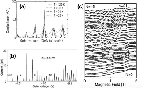
(34) (a). (c). (b). Fig. 1.4. Experiments related to the Coulomb blockade effect. In (a) the electrical conductance is plotted as a function of the gate voltage applied in a QD setup showing a series of equidistant resonances which smear out at higher temperatures. This picture is taken from Y. Meir et al. [14]. In (b), Kouwenhoven et al. [16] found the same series of peaks separated due to the electron-electron interactions. Finally, (c) shows the evolution of the peaks maxima as function of a magnetic field reported by Ciorga et al. [19].. Vg with a smearing at higher temperatures (Fig. 1.4a). Kouwenhoven et al. [16] also reported CB oscillations as shown in Fig. 1.4b and applied the orthodox model to explain this phenomenon . Additionally, they found a staircase in the current I due to the addition of electrons to the discrete levels of the QD. Nagamune et al. [17] observed similar results in a QD which also exhibits Coulomb oscillations. Tarucha et al. [18] studied the modification of these oscillations when a magnetic field is applied. The CB resonances shift in pairs when a magnetic field is applied. The latter is strongly related with the results of Sec. 7.2. Ciorga et al. [19] studied the transport in a lateral QD under magnetic fields (Fig. 1.4c) obtaining a spin-blockade effect making it possible to find the spin state by measuring the current. These are just a few representative examples. The list we provide is by no means exhaustive. The CB effect is a main topic of this thesis and we will discuss it properly in the results. First, we analyze the CB effect and the thermoelectric properties (see Sec. 3 for more information about thermoelectricity) of a single QD model in Sec. 7.1. Later, we closely examine the difference between interacting and noninteracting molecular junctions (more information about these systems in Sec. 1.2) in Sec. 7.2. Finally, we investigate the role of interactions in parallel-coupled DQD in Sec. 8.1.. 8. Quantum dots.

(35) 1.2. Molecular junctions As explained previously, QDs are not the only system exhibiting CB features. This section concerns molecular junctions, systems where a molecule controls the electronic transport between metallic reservoirs. Additionally, these systems have characteristics similar to QDs. We can classify these devices within a branch of science called molecular electronics [20], which investigates electrical and thermal transport of individual molecules or combination of them. This area emerged several decades ago with a change of the perspective for molecules: They were not only part of bulk materials, but they might also be useful components for the electronic industry. Nowadays, the analytical tools and device architectures have motivated many scientists from different disciplines to join efforts in this interesting field. Molecular electronics is important mainly for two different reasons. First, the implementation of molecular devices into nanoelectronic systems serves as a complementary tool due to their novel functionalities out of the scope of solid state devices. On the other hand, it offers new fascinating physics in the description of how molecules behave out of equilibrium. Concerning technological aspects of molecular electronics, it has good advantages in comparison with the technology of regular transistors [21]: To start with, the size of the molecules is around 1 or 10 nanometers and provides good benefits in terms of cost and efficiency. Another advantage is the speed of the molecules because conduction may be favored in well-fabricated molecular wires. Additionally, the fruitful improvement in the technology of nanodevice manipulation makes both the self-assembly of molecular structures and the tuning of its electrical properties easier. Finally, the large number of molecule structures yield new technological insights which a usual silicon-based technology may not achieve. The first notion of molecular electronics appeared in the 1950’s by Arthur von Hippel introducing the basis of bottom-up approach as molecular engineering [22]. However, molecular electronics really started in the late 1960’s when several groups studied experimentally the electric transport through molecular monolayers. During the 1970’s Aviram started the theory of electron transfer in single molecules. In fact, he gave the first proposal of using a single molecule as an electronic component called molecular rectifiers [23]. A huge progress occurred in the 1980’s with the invention of the scanning tunneling microscope (STM). In fact, the first molecular electronic device appeared in 1985 [24]. More recently, two different groups reported the first transport experiment in single molecule junctions [25] in 1997, which helped molecular electronics to become a well-established field.. Quantum dots. 9.

(36) The fabrication process of molecular junctions is based on the creation of an atomic-sized contact into a metallic layer. In such contact the molecule shall be placed allowing transport through it. There are different ways to perform it: Employing an STM or an atomic force microscopy (AFM) in which the gap is created using a tip and they move electrons via tunnel currents or electrical forces, respectively. Notwithstanding, one of the most used fabrication processes is the electromigration technique. The method consists of the assembly of a wire between metals which is burnt by applying strongly electrical currents (see Fig. 1.5c). Then, the wire breaks yielding a nanoscale gap inside which the molecule may be stacked. The fabrication of tunnel junctions explained previously provide setups where the molecule acts as a SET. The molecule energy levels permit a sequential tunneling in the transport where only a single electron may flow though the system at the same time. Nevertheless, there are different molecular systems in tunnel junctions. For example, we highlight the STM break-junctions [26, 27]: the molecule is attached to a metal reservoir and the tip of a STM. A voltage difference is applied between components giving rise to an electrical current through the molecule. Finally, self-assembled molecules (SAM) are also common examples of systems composed of molecular tunnel junctions [28, 29, 30, 31, 32, 33]. They consist of domains where molecules spontaneously organize on top of a metal generating a surface. To induce currents, another metallic material is connected on top of these SAMs.. 1.2.1. Transport in molecular junctions We now briefly review the state of the art in transport experiments concerning molecular junctions. First, H. Park et al. [34] reported transport measurements in molecular SETs. The current through the molecule presented quantization of the molecular levels and at low voltages the conductance was surpressed obeying the Coulomb blockade effect (see Fig. 1.4b). Later, J. Park et al. [35] showed additional results for SET for two different molecules. They also observed CB effects as the previous work. For strong interactions, a zero-bias anomaly appeared in the electrical conductance as a signature of Kondo correlations (for more information about the Kondo effect, see Ch. 2). The conformation of a molecule in a tunnel junction has been demostrated to modify the shape of the electrical conductance. Venkatamaran et al. [26] reported that the conductance decreases as the twist angle between phenyl units in a biphenyl molecule increases. They also observed a decrease of conductance with the number of phenyl units in the molecule. Similar results were found by Ho Choi et al. [36] (Fig. 1.5a). They studied the. 10. Quantum dots.

(37) (a). (b). (c). Fig. 1.5. (a) Resistance versus the length of a molecular wire. Increasing the length of molecule will increase its resistance and, consequently, the electrical conductance will decrease. Figure extracted from Ho Choi et al. [36]. (b) Current as a function of the voltage bias of a DNA molecule with different lengths. This is a clear example of a molecule diode. This image is a slight modification of Livshifts et al. [39]. (c) Images showing a junction during an electromigration process. Clearly, in the fourth image the junction is broken and a small constriction has been created. This image is taken from Cuevas et al. [20].. resistance of a molecule dependent on its length finding an increase at higher lengths. More concretely, they found transport regimes for short and long molecules. For each of these regimes, the resistance increases with different exponential trends. The length dependence of the electrical conductance was also studied by Lafferentz et al. [37]. Interestingly, the I − V characteristics exhibit a molecular diode shape. Graphene nanoribbons seems to show a similar length dependence in transport than previous works as Koch et al. reported [38]. Surprisingly, DNA molecules also exhibit molecular diode characteristics as explained by Livshifts et al. [39] (see Fig. 1.5b). In addition to the molecular diode characteristics, Yan et al. identified three different regimes depending on the thickness of a molecule. At low thickness, the coherent tunneling controls the electrical current. On the other hand, strong temperature dependence and hopping transport appear for large thickness. Finally, for intermediate thicknesses (around 3 − 20 nm) the electric current is tuned mainly by the voltage bias. Yuan et al. [40] concluded that control of the coupling between molecules and electrodes is essential to the fabrication of molecular junctions. They found high rectification ratios when a ferrocene. Quantum dots. 11.

(38) SAM is strongly coupled to the electrodes. Similar rectification effects were also detected by Chen et al. [31]. They attributed the rectification to Coulomb interactions which permits to switch electrostatically the coupling between molecules and electrodes. Concerning thermal effects, Garrigues et al. [41] investigated the temperature dependence of a Ferrocene molecule. They identified several transport regimes which behave quite differently when temperature is increased. They fit the results using a model which does not take into account electron-electron interactions. A more detailed explanation of the work of Garrigues et al. [41] is found in Sec. 7.2.1. We will compare such work with an interacting model which is also able to fit the experimental results (Sec. 7.2.2). In Sec. 7.2.3, we will discuss the possibility of distinguish between noninteracting and interacting cases. Finally, for a more general overview of molecular junctions one can read Refs. [20, 33, 42].. 1.3. Double quantum dots Since QDs can be considered as artificial atoms, the condensed matter analogue of the molecule is the DQD. They consist of a combination of two QDs which can be connected between them with a tunnel amplitude or capacitively (via Coulomb interactions). DQDs are fascinating devices which exhibit rich physics to be still understood and, consequently, they are one of the pillars of this thesis. Applying the fabrication techniques explained previously, the creation and manipulation of DQDs are as straightforward as the single QD becoming a suitable device to investigate quantum coherence and superposition states. In addition, there are multiple DQD structures depending on the tunnel configuration between the different parts of the setup (the reservoirs and the dots). Generally, we can distinguish two clear configurations: Parallel-coupled DQDs (Fig. 1.6a) where the QDs are connected to the same reservoirs, usually with a low dot-dot tunnel amplitude, and serially-coupled DQDs (Fig. 1.6b) where each dot is coupled to only one reservoir and electrons have to cross both dots in order to generate transport. In addition to the Coulomb blockade effect caused by intradot couplings, we find that the electron-electron interaction between the dots (interdot) may be also significant in the electronic transport. An electrostatic model similar to the Sec. 1.1 is used in order to obtain the stability diagram of the system, i. e. , the regions of (Vg1 , Vg2 ) where the number of electrons occupying the dots is increased or decreased by one unit (ni → ni ±1 where i = 1, 2 is the subindex determining the QDs). Fig. 1.6c shows the most general electrostatic model for a DQD system, each dot. 12. Quantum dots.

(39) Vg2 (a). (c). QD1. Left Lead. Right Lead. Cg2 RL2 , CL2. RR2 , CR2. VL2. VR2. QD2. Rt , C t. (b) Left Lead. RL1 , CL1. QD1. QD2. Right Lead. RR1 , CR1. VL1. VR1 Cg1 Vg1. Fig. 1.6. Schematics of the structure of a parallel-coupled DQD (a) and a seriallycoupled DQD (b). The former consists of two QDs coupled to the left and right electronic reservoirs while in the latter each dot is attached to a single reservoir and the opposite QD. (c) General sketch of a DQD electrostatic circuit: The tunnel coupling between the reservoir α = L, R and the dot i = 1, 2 is modelled with a resistance Rαi and a capacitor Cαi . The dot-dot coupling is represented by Rt and Ct . Additionally, the QD levels may be tuned by applying gate voltages Vgi .. attached to two reservoirs with tunnel and capacitive couplings characterized by a resistance Rαi and a capacitance Cαi where α = L, R denotes the reservoir. Besides, a voltage Vαi may be applied to each reservoir of the system. The tunnel barrier between dots is characterized by Rt and Ct . For interacting dots without tunneling, the resistance is assumed to be large Rt → ∞. Finally, the QDs level positions are tuned with the gate voltages Vgi . With this model one can switch from the serial to the parallel configuration just with an appropriate change of the parameters of the system.. 1.3.1. Parallel configuration When both dots are connected to the reservoirs but with small tunneling between dots such as Rt ≪ RL1 , RL2 , RR1 , RR2 in Fig. 1.6c, we deal with the parallel configuration (Fig. 1.6a). In an electrostatic circuit the system is usually described when VL1 = VL2 and VR1 = VR2 (see Fig. 1.6c). The stability plot of the parallel DQD clearly shows hexagonal shape (Fig. 1.7a) [43, 44]. Generally, the occupation of the QDs only varies by one electron in sequential tunneling (gray lines in Fig. 1.7a). However, cotunnel transitions are also possible in which two electron transitions take place simultaneously (red lines in Fig. 1.7a). This configuration is interesting because electrons may take multiple possible paths the transport leading to a coherent superposition of them.. Quantum dots. 13.

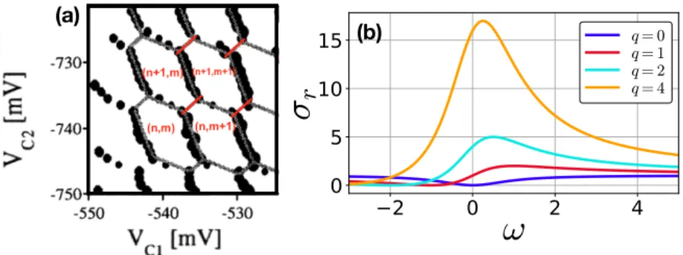
(40) (a). (b). Fig. 1.7. (a) Stability diagram for a typical DQD, VC1 , VC2 are the gate voltages applied to the dot 1 and 2, respectively. The plot data represent experimental values while the solid lines display the expected diagram computed from an electrostatic model. The solid red lines show the region where a cotunnel transition may occur modifying (n + 1, m) → (n, m + 1), n and m being the occupation of the first and second QD. This is a simultaneous two-electron transition. This plot is a slight modification of a figure taken from Hofmann et al. [43]. (b) Ratio of transitions probabilities of a particle between the unperturbed path of a continuum state and the perturbed path due to a discrete level as a function of the energy ω and different values of the Fano parameter q [Eq. (1.8)] in a DQD setup.. We now briefly discuss coherence induced effects: • Aharonov-Bohm (AB) Interferometer. DQDs can act as AB interferometers [45]. These devices [46] are systems where an electron can travel in two different ways (in a DQD setup, each possible path crosses a QD) from left to right reservoir. Electrons display an interference pattern dependent on the phase difference between paths. The coherence strongly depends on the singlet or triplet states of a pair of electrons flowing through the AB interferometer [47]. Due to the AB phase, the electric conductance of the system exhibits oscillations when the magnetic field is tuned [45, 48, 49]. • Fano resonances. Among the interference phenomena which may manifest themselves in DQDs, we highlight the appearance of Fano resonances [50, 51]. They are produced due to the existence of a coupling between continuum and discrete quantum states [52]. Therefore, particles may perform two different transitions during transport: a path which starts at the continuum, moves to the discrete state and then returns to the continuum and a second one where carriers are not perturbed by the discrete state. The interference between these two amplitudes creates asymmetric line shapes in the total density of states or transmission of the system. In order to observe the asymmetric lineshape, we calculate the ratio σr between the total and the unperturbed transition probabili-. 14. Quantum dots.

(41) ties as a function of the energy ω and the Fano parameter q obtaining, σr =. (ω + q)2 . 1 + ω2. (1.8). We plot this ratio for different Fano parameters q in Fig, 1.7b. We observe that when q = 0 the curve is symmetric and has an antiresonance at ω = 0. As q increases, the shape of the curve becomes more asymmetric. These antiresonances will be also shown in the transmission function of a DQD denoting the existence of a bound state in the continuum (BIC). The DOS ρ(ω) is now split into two different components: a continuum function of the global spectrum and a discrete state indicated as a Dirac delta centered at the BIC position ω0 : ρ(ω) ≈ f (ω) + δ(ω − ω0 ). In Ch. 8.1, we will explain how BICs are influenced by Coulomb interactions and will discuss their electric and thermoelectric effects. • Dicke effect: Following with the coherence related effects, the Dicke effect resembles the Fano effect in similar ways [53]. This effect was first explained in the context of collisions of atoms in a solid [54]. Dicke states that Doppler resonances which result from the change of momentum due to spontaneous emission of a photon in a pair of atoms generate a resonance in the DOS which narrows in the absence of collisions. In comparison with the Fano effect, the Dicke effect is its optics analogue. Since impurities in metals and QDs can be treated as artificial atoms, the Dicke effect is also expected to arise [55, 56]. Additional effects can be found in parallel-coupled DQDs. For instance, Coulomb drag in QDs, a topic which will be deeply explained in Sec. 1.3.2, is a very appealing effect which has attracted lots of attention nowadays. Furthermore, an experiment was performed by Holleitner et al. [57]. They reported that cotunnel effects between dots occur without Coulomb charging energies (strongly related with Fig. 1.7a) and they found that by increasing the interdot tunneling the conductance resonances start to merge. Fuhrer et al. [58] reported Fano effect mesurements due to magnetic fluxes and high temperatures. They discovered vanishing Fano resonances at high temperatures. They were able to tune the asymmetry with a magnetic field. Additionally Gustavsson et al. [59] were able to detect in real-time electrons interfering in DQDs using a quantum point contact (QPC) as a charge detector. A promising application of DQD setups is their functionality to work as qubits in a quantum computer [60, 61, 62] due to their entanglement properties and easy manipulation using quantum gates.. Quantum dots. 15.

(42) 1.3.2. Coulomb drag A special case of a parallel DQD structure is described by VL1 = VR1 = 0 and Rt → ∞ in Fig. 1.6c yielding the Coulomb drag effect [63]. In this setup we distinguish two different subsystems coupled to each other via an interdot Coulomb interaction between electrons occupying the QDs described by the capacitance Ct in the electrostatic model. Coulomb drag is just one particular case of a broader topic known as the frictional drag. The phenomenon consists of two isolated conductors with a small separation: one conductor is driven out of equilibrium by an applied voltage V which induces an electric current through this active conductor. However, the passive system is also affected by the bias V of the active layer although this second system is at equilibrium. An interaction between the carriers of the passive and active layers triggers the generation of current at the equilibrium system. In other words, carriers in the biased system drag carriers in the equilibrium system exchanging energy and momentum. The interaction can be of any kind: electronphonon [64], plasmon [65] or Coulomb interactions, the latter being the main interest in this thesis. Concerning conductors, the Coulomb drag appears in a variety of systems such as 2DEGs [66], nanowires [67], graphene heterostructures [68], etc. We focus our attention on a capacitive-coupled DQD as sketched in Fig. 1.8a: each layer is composed of a QD attached to two reservoirs. The reservoirs of the active layer (drive system) are at different electrochemical potential generating a voltage bias V . In contrast, the leads of passive layer (drag system) remain at the Fermi energy εF . The interaction between layers is basically an interdot electron-electron interaction Ũ . The main cause of the induced current in this nanodevice is an asymmetry in the drag system as reported by Sánchez et al. [69]. They showed that the detailed balance condition has to be broken in order to find mesoscopic drag in the DQD system. This prediction was confirmed experimentally by Shinkai et al. [70] and later by Bischoff et al. [71]. In essence, the asymmetry arises from different tunnel coupling of the drag QD to the leads (RL1 ≠ RR1 and CL1 ≠ CR1 in Fig. 1.6.). Recent theoretical and experimental works [71, 72, 73] reveal that cotunnel processes, in addition to sequential tunneling, are crucial to characterize the generation of drag currents. Several theoretical discussions of the drag effect have recently appeared. Jauho and Smith [74] analyzed the mesoscopic drag current between two 2D conductors for diverse background temperatures. They solved the Boltzmann equation with the goal of examining the change of momentum between layers. They found that the momentum transfer depends on T 2 , in good agreement with previous experimental works. 16. Quantum dots.

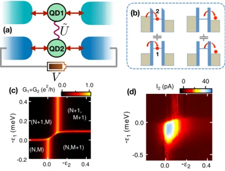
(43) QD1. (a). (b). 2. Ũ QD2. 1. V (c). (d). Fig. 1.8. (a) Scheme of a capacitive-coupled DQD acting as a Coulomb drag system. QD1 is attached to the top reservoirs at equilibrium while the QD2 is attached to leads with a voltage difference V . The QDs are linked with an electron-electron interaction Ũ when both dots are filled with one electron. The top system reacts to the applied bias of the bottom system with an induced current at a preferential direction depending on the tunneling amplitudes. (b) Energy diagram of the dominant cotunnel processes yielding drag currents. The height is associated to energy values. Left and right brown squares indicate the lead density of states denoted as Fermi seas controlled by the eletrochemical potentials. The lines in the middle represent the QD energy level taking place in the cotunnel process. Image extracted and slightly modified from Keller et al. [72]. (c) Experimental stability diagram portraying the number of electrons of the drive N and drag M QDs. (d) Experimental measurements of drag current as a function of the drive ε1 and drag ε2 levels for a given electrical bias. One can observe a regime where the drag takes place around the triple points indicated at (c). Images (b), (c) and (d) are extracted from Keller et al. [72].. [75]. Kamenev and Oreg [76] reported results of drag physics in 2D nanodevices finding a rectification of the thermal fluctuations due to the electric fields of the drive system. Levchenko and Kamenev [77] examined exhaustively the drag mechanism in a quantum circuit formed by two QPCs coupled capacitively. The drag is produced by asymmetries in the energy-dependent transmission probabilities of the QPCs. In the linear regime of voltage bias, they observed that the device behaves like a bulk 2D system and in the nonlinear regime, the drag is attributed to the shot noise of the active layer. Later, Sanchez et al. [69] studied fluctuation-dissipation relations emphasizing that they are still satisfied. Quantum dots. 17.

(44) despite the violation of the detailed balance condition. We want to stress two papers published almost simultaneously: Kaasbjerg and Jauho [73] and Keller et al. [72]. Both of them used a master equation approach (for more information about the theoretical model see Segal [78]) obtaining similar theoretical results. They reported that lowest order cotunnel transitions, i. e. , transitions for one electron going out of (into) the drive QD while simultaneously another electron goes into (out of) the drag dot (Fig. 1.8b), play an important role in the Coulomb drag of DQDs. In accordance with previous reports, energydependent transition probabilities are also needed in order to generate drag. Particularly, Keller et al. showed measurements of a capacitively DQD setup for interdot interactions larger than the lead tunnel rates. They observed that the drag current is higher around the triple points (Fig. 1.8c) corresponding with the range of parameters where the cotunnel transitions take place. In Sec. 8.2, we also investigate theoretically the Coulomb drag effect in a DQD setup using the Keldysh nonequilibrium Green’s function formalism (Ch. 4). We obtain good agreement with the previous experimental results. We connect the Coulomb drag effect with the orbital Kondo effect (for more information see Sec. 8.2) giving some qualitative predictions. Finally, we would like to emphasize the applicability of the Coulomb drag in the current technology. Since DQDs are good candidates for quantum information and quantum computing, the drag effect allows us to analyze deeply and detect the transport mechanism through qubits.. 1.3.3. Serial configuration Now, we consider the case of RL1 , RR2 → ∞ and CL1 , CR2 → 0 in the circuit of Fig. 1.6. Notice that carriers need to cross both dots in order to generate non-vanishing currents. Thus, for disconnected dots (Rt → ∞), transport is prohibited. This corresponds to the serial configuration of QDs. At low voltage bias, the stability diagram for serial DQDs is similar to the one shown in Fig. 1.7a also exhibiting an hexagonal shape when tuning the gate voltage of the dots [79]. For dots with a single level ε1,2 contributing to transport, the energy levels of the artificial molecule can be expressed in a more convenient form for negligible interdot Coulomb interactions (Ũ → 0). Thus, we obtain a superposition of bonding and antibonding states: √ ε1 + ε2 ε1 − ε2 2 ε± = ± ( ) + ∣τ ∣2 , (1.9) 2 2 where ε− (ε+ ) is the bonding (antibonding) energy level and τ is the tunneling amplitude for an electron to hop between QDs. Notice that. 18. Quantum dots.

(45) we have two energy levels separated at least by τ . Therefore, unless the DQD is decoupled (which makes no sense because we would be dealing with two single QDs systems), the bonding and antibonding levels will never cross. Anyway, for separated energy levels ∆ε = ε1 − ε2 ≫ τ the tunnel amplitude would be negligible. Another intriguing effect may be encountered when we include spin effects in a highly interacting serial DQD system with also high tunneling amplitudes. At large intradot interactions such that only one electron is occupying each dot, the system yields a superexchange interaction Jex ≈ τ 2 /U which connects the electron spin of the dots. In this situation, the DQD states turns out to be singlet and triplet states. The former would be the ground state [61, 80] which allows the detection and control of the electron spin with a simple detuning the dot energy levels [81]. This result has fundamental importance for quantum computation [60] because serially-coupled DQDs are prototypical examples of entangled qubits. In fact, a large variety of discussions about quantum computation in serial DQDs have been reported [62, 82, 83]. Furthermore, electrons in a serial DQD may also interact with the electron spins at the leads yielding two-impurity Kondo systems. This topic will be explained carefully in Ch. 2. In the thesis we discuss transport in serially-coupled DQDs in Sec. 8.3 for low temperatures leading to the Kondo effect. We study the thermoelectric and heat transport of a two-impurity Kondo system observing that the thermal bias is able to decouple the DQD. We also investigate how the superexchange interaction Jex is modified by these thermal differences.. Quantum dots. 19.

(46) 20. Quantum dots.

(47) 2. Kondo effect Condensed matter physics harbors mysteries and unknown questions yet to discover. It deals with structures embedded in metals, which contain a large number of particles. Since these particles are charged, interactions take place over the whole structure. Therefore, although some effects may be well understood with statistical and mean-field methods, the evidence that there exists complexity in metals is indisputable. The field is thus a part of many-body physics. As an example, a many-body physics problem might be the Coulomb blockade already explained in Sec. 1.1 because even though Coulomb interactions involve two particles, the screening effect of an occupied QD clearly influences all electrons flowing through the leads. On the other hand, when we consider spin and magnetic impurities, metals may experience a very intriguing phenomenon: The Kondo effect [84]. We understand magnetic impurities as the ones which contribute with a Curie-Weiss term to the susceptibility X = C(T + θ̃)−1 where C is the Weiss constant and θ̃ is a constant temperature. Basically, the impurities have localized spins which may interact with free conduction electrons in the metal. The spin interactions are responsible of multiple transport phenomena. The most clear manifestation is the appearance of a minimum in the resistance at low temperatures. The first observation of this phenomenon was made by de Haas et al. [85] in 1934. However, no rigurorous theoretical explanation appeared until 30 years later when Kondo published his theory [86]. After Kondo’s work, the effect behind the resistance minimum was still a topic of discussion for 30 more years since the effect was not totally understood in all regimes of temperature. It turns out that the birth of nanotechnology inspired a revival of the subject during the last decades [87]. The possibility of simulating the behaviour of magnetic impurities using a QD [7] opens a new window to test the Kondo effect experimentally, spurring a growing interest in theoretical research. Additionally, the easy manipulation of the relevant parameters of a nanodevice enables features and phenomena that would be unfeasible to examine with normal metals. In this chapter, we explain what the Kondo effect is and discuss the state of the art of this paradigmatic effect. More concretely, we describe. Kondo effect. 21.