Do climate variations explain bilateral migration? A gravity model analysis

Texto completo

(1)Backhaus et al. IZA Journal of Migration (2015) 4:3 DOI 10.1186/s40176-014-0026-3. ORIGINAL ARTICLE. Open Access. Do climate variations explain bilateral migration? A gravity model analysis Andreas Backhaus1†, Inmaculada Martinez-Zarzoso2,3*† and Chris Muris4† * Correspondence: [email protected] † Equal contributors 2 University of Goettingen, Platz der Göttinger Sieben 3, 37073 Göttingen, Germany 3 Universidad Jaume I, Castelló de la Plana, Spain Full list of author information is available at the end of the article. Abstract: This paper investigates to what extent international migration can be explained by climatic variations. A gravity model of migration augmented with average temperature and precipitation in the country of origin is estimated using a panel data set of 142 sending countries for the period 1995 to 2006. We find two primary results. First, temperature is positively correlated with migration. Second, stronger changes in precipitation are also associated with aligned, but small changes in migration. Both effects are robust to various model modifications. Furthermore, we present initial explorations into the channels relating climate changes with migration via agriculture and internal conflict. JEL Codes: F22, Q54 Keywords: International migration; Climate change; Gravity model; Panel data. 1. Introduction The nexus between climate change and migration has been addressed since the early 1990s by political scientists, environmentalists and demographers. In particular, the discussion intensified after the release of the conclusions of the Fourth Assessment Report of the Intergovernmental Panel on Climate Change (2007). The report refers to the “potential for population migration” due to climate distress. The topic has received substantial media coverage but limited academic research. Although a number of recent policy publications are concerned with the impacts of climate change on migration, most of them are case studies for specific regions/countries and time episodes. Surprisingly, only few empirical studies attempt to quantify this impact on a larger scale. While the standard statistical migration literature examines socioeconomic drivers of bilateral migration without considering climate factors at all, at least a number of recent studies focuses on natural disasters and extreme events as drivers of migration (e.g., Warner et al. 2009). In this paper, we focus on permanent emigration due to gradual changes in climate. We follow the approach by Dell et al. (2008), but our outcome variable is emigration instead of economic growth. The main aim of the paper is to derive estimates of the effect of changes in climate variables, namely temperature and precipitation, on migratory flows from 142 countries of origin into 19 OECD countries over time and across countries. In particular, we estimate a gravity-type model augmented with climate variables while controlling for the established socioeconomic factors. © 2015 Backhaus et al.; licensee Springer. This is an Open Access article distributed under the terms of the Creative Commons Attribution License (http://creativecommons.org/licenses/by/4.0), which permits unrestricted use, distribution, and reproduction in any medium, provided the original work is properly credited..

(2) Backhaus et al. IZA Journal of Migration (2015) 4:3. The main results show that an increase in temperature significantly correlates with a higher migration flow between a country pair. Changes in precipitation are also positively and significantly correlated with migration, but to a lower extent. These findings are robust to various model modifications. Furthermore, emigration from more agriculturally-dependent countries appears to be related to changes in temperature only, while less agricultural countries are merely affected by precipitation changes when it comes to emigration. A state’s internal fragility on the other hand seems to have a direct effect on emigration, but no significant interaction with climate change. The rest of the paper is structured as follows. Section 2 reviews the literature on bilateral migration and climate change. Section 3 refers to the related theoretical models and derives the main empirical specification. Section 4 presents the empirical application, the main results, our robustness checks, as well as the explorations into two potential channels between climatic variations and migration. Section 5 concludes.. 2. Literature review We distinguish between existing studies focusing on the more general socioeconomic determinants of international migration on the one hand and more specific ones adding climate and environmental variables on the other hand. Within the first category, studies on migration from many origins to many destinations include Mayda (2010), for 79 countries of origin to 14 OECD countries over the period 1980–1995, and the more recent Ruyssen et al. (2014), who investigate the determinants of bilateral migrant flows to 19 OECD countries between 1998 and 2007 from both advanced and developing countries of origin. In general, they find solid evidence for the importance of economic differentials between the sending and the host countries. It is notable that among the works focusing on the impact of climate and environmental factors on migration, the majority of them put an emphasis on natural disasters rather than climate trends as potential push factors. An overview of this literature can be found in Belasen and Polachek (2013). Naudé (2009) studies the determinants of emigration from 43 African countries of origin, excluding bilateral migration, over 5-year intervals during the period 1960–2005. The main environmental measure used is the sum of weather and seismic disasters in the respective country of origin, which is found to increase emigration. Using bilateral migration data, Reuveny and Moore (2009) cover emigration from 107 countries to 15 OECD host countries over the period 1986–1995. However, only weather-related disasters and the area of crop and arable land are used as proxies for climate change. Aside disasters, crop land is found to have a significantly positive effect on emigration, which the authors interpret as an indication of distributional conflicts within developing sending countries. A paper closely related to our work is the gravity study by Afifi and Warner (2008) that estimates a gravity model augmented with thirteen environmental factors, which in general have a significant and positive impact on migration. Its main shortcoming is that all the environmental factors are modeled as “event” dummy variables taking the values zero or one without accounting for the magnitude of the factors. Further, only a single cross-section of data is employed. We depart from these approaches by focusing on within-country variation in temperature and precipitation and hence take into. Page 2 of 15.

(3) Backhaus et al. IZA Journal of Migration (2015) 4:3. Page 3 of 15. account the changes over time in both factors. In addition, the panel structure of our data also allows us to rectify the potential problem of unobserved heterogeneity across countries. Finally, Beine and Parsons (2013) consider both natural disasters and climatic variations as potential drivers of bilateral migration flows. However, their data provide information on migration in ten year intervals only, which is why their analysis is oriented towards medium- and long-run effects of climate volatility. Their results do not show any direct effect of the latter on international migration flows.. 3. Theoretical background and model specification Our benchmark specification is a gravity model augmented with climate variables. The non-climate control variables in the gravity model are derived from neoclassical theory, namely economic, demographic, geographic and cultural controls, as well as the tradeto-GDP share: lnM ijt ¼ αo þ α1 wtempit þ α2 wpreit þ α3 GDP it þ α4 GDP jt þ α5 DemPresit þα6 lnPopulationit þ α7 U jt þ α8 Tradeit þ γ t þ ωij þ εijt;. ð1Þ. where Mijt denotes migration inflows from country i to country j in year t. A frequently used alternative to the logarithm of migration flows is the emigration rate, which is defined as the flow of population from country i to country j in year t divided by country i’s population in year t. However, it is not identifiable whether changes in the emigration rate over time arise from changes in the migration flows, changes in the population size aside from emigration, or both. Therefore, the logarithm of the migration flows is used as the dependent variable while controlling for general population dynamics by including the logarithm of the emigration country’s population. The population‐weighted average annual temperature in degrees Celsius is denoted wtempit, while wpreit denotes average annual precipitation in millimeters. The idea behind using population weights is to make the climate data reflect more precisely how strongly the inhabitants within a given country are actually affected by variations in temperature and precipitation, following the approach proposed by Dell et al. (2014). GDPit (GDPjt) denotes PPP-adjusted GDP per capita divided by a factor 1000 in the origin (destination) country in year t. A squared term of GDPit is also included in all specifications to account for non-linear effects of income in the origin country. DemPresit denotes the share of young people in the country of origin’s working age population. Ujt denotes the unemployment rate in the country of destination at time t, which controls for the absorptive capacity of the receiving country’s labor market, while Tradeit denotes the openness ratio, (Exports + Imports)/GDP, in the country of origin at time t. The term ωij captures country-pair characteristics, while a set of year dummies γt captures global shocks. Finally, εijt is the error term.. 4. Empirical application 4.1 Data and variables. Data on yearly average temperature and precipitation in the countries of origin stem from Dell et al. (2008) and cover the period 1995–2006, yielding 12 time periods for.

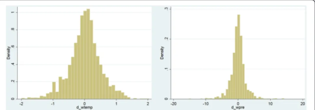
(4) Backhaus et al. IZA Journal of Migration (2015) 4:3. our analysis1. The authors aggregate both variables to the country-year level. The variables they use are population-weighted averages using 1990 population figures. Figure 1 presents histograms of the changes in average temperature and precipitation in our sample. While we can accept the hypotheses that the means of the two distributions are greater than zero, the distributions are more centered than one might expect in the context of climate change. Further, the majority of the yearly changes appear to be rather subtle, as only 5.4% of the temperature changes in our sample fall outside the interval [−1, 1] degree Celsius, and 1.65% of the changes in precipitation fall outside the interval [−5, 5] millimeters. Figure 2 depicts the average changes in temperature and precipitation globally (i.e., pooling observations from all countries of origin in the sample) over time. While the two series exhibit a strong negative correlation, their volatility around the pooled global mean of all sending countries and all time periods decreases considerably after the year 2000. The corresponding data on yearly migration flows from source to destination countries originate primarily from the OECD’s International Migration Database (IMD, 2014). We select 19 OECD members as destination countries on the basis of data availability, while examining inflows from 142 countries of origin. Some of the latter are members of the OECD as well, e.g., Mexico. Although Mexico might be an important destination country itself from the perspective of less developed countries, its role as a sending country is probably more important in our context. A complete list of the source and destination countries together with their respective share of non-missing migration flow observations can be found in Table 5 in the Appendix. The IMD is constructed on the basis of statistical reports of the OECD member countries, which implies that the data might not be fully internationally comparable as the criteria for registering population and the conditions for granting residence permits vary across countries. Illegal migration flows are only partially covered as data are only obtained through censuses. Further, the majority of the countries of destination did not record immigrants from the full set of source countries during the first few years of our period of analysis; thus, missing data are most frequent in this period. In the cases of Japan and the Republic of Korea, only the inflows from the most important regional sending countries have been recorded over a longer period of time. Regarding the European destination countries, data on inflows into Italy are missing for many source countries and is completely unavailable for the years 1995–1997 and 2003. Fortunately, we were. Figure 1 Changes in average temperature and precipitation.. Page 4 of 15.

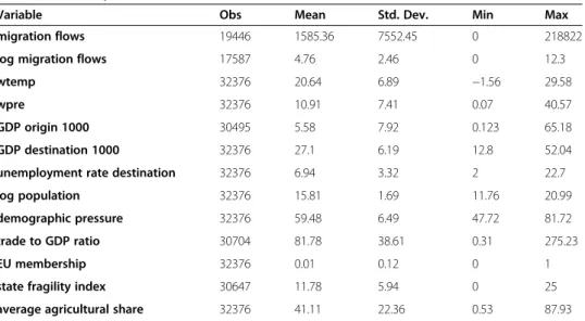
(5) Backhaus et al. IZA Journal of Migration (2015) 4:3. Figure 2 Global volatility in average temperature and precipitation.. able to fill some of the gaps with observations from the Eurostat online database (Eurostat 2014). For Austria, Switzerland, and the UK, numerous non-European source countries could be added. Moreover, some rounded and inaccurate figures for the UK could be replaced. Adding and replacing rounded observations was only done if the figures from the OECD and the Eurostat databases coincided for countries for which data are available in both databases. In this way, we can be relatively sure that the same definitions of immigration are used in both data sources and that the consistency of our dataset is not compromised by combining them. However, the Eurostat data collection starts only in 1998, so that previous years remain unchanged. The data are predominantly complete for France, Spain, and Germany though, which together absorb about 60% of the migratory flows to Europe in our sample. Data from Australia, Canada, and the United States cover inflows from almost all source countries for all or nearly all time periods, reflecting the long history of immigration in these countries. With 12 years, 142 countries of origin, and 19 countries of destination, we would obtain a maximum of 32,376 observations. However, 13,190 of the observations remain missing. But we can claim to have obtained a dataset as comprehensive as possible of immigration to OECD countries by combining OECD and Eurostat information where it was possible. The evolution of the migration flows from the perspective of the receiving countries is depicted in Figure 3. Data for the economic and demographic variables are obtained from the World Bank’s World Development Indicators (WDI 2014) database. Table 1 presents summary statistics of the main variables included in our model.. 4.2 Estimates of the static model. The augmented gravity model introduced in Section 3 is estimated for a sample of 142 origins and 19 destinations over the period 1995 to 2006. In our empirical model, we allow the country-pair effects ωij to be correlated with the explanatory variables. Possible reasoning behind this assumption is, e.g., that each destination country has its own unobservable, time-constant mentality towards immigration that affects actual immigration flows, or that there exist specific stable relations between some source and destination countries. The country-pair unobserved heterogeneity could be controlled for by applying a transformation that eliminates the time-invariant effects, such as the fixed effects (FE) or the first differences (FD). This would also wipe out any unilateral. Page 5 of 15.

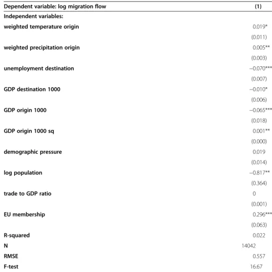
(6) Backhaus et al. IZA Journal of Migration (2015) 4:3. Page 6 of 15. Table 1 Summary statistics Variable. Obs. Mean. Std. Dev.. Min. Max. migration flows. 19446. 1585.36. 7552.45. 0. 218822. log migration flows. 17587. 4.76. 2.46. 0. 12.3. wtemp. 32376. 20.64. 6.89. −1.56. 29.58. wpre. 32376. 10.91. 7.41. 0.07. 40.57. GDP origin 1000. 30495. 5.58. 7.92. 0.123. 65.18. GDP destination 1000. 32376. 27.1. 6.19. 12.8. 52.04. unemployment rate destination. 32376. 6.94. 3.32. 2. 22.7. log population. 32376. 15.81. 1.69. 11.76. 20.99. demographic pressure. 32376. 59.48. 6.49. 47.72. 81.72. trade to GDP ratio. 30704. 81.78. 38.61. 0.31. 275.23. EU membership. 32376. 0.01. 0.12. 0. 1. state fragility index. 30647. 11.78. 5.94. 0. 25. average agricultural share. 32376. 41.11. 22.36. 0.53. 87.93. Note: w indicates that the corresponding variable is population-weighted.. country fixed effects that might influence the migration decision, e.g., a country’s access to the sea. In the following, our preferred estimation procedure is the FD estimator. The FE estimator is consistent if current variations in our explanatory variables are uncorrelated with past, present, and future error terms in our migration flow specification (1). However, cross-country panel data with fixed T typically exhibit a high degree of autocorrelation, which in turn makes the requirement for a consistent FE estimate less likely to be met. The FD estimator is consistent under the less restrictive assumption that changes in the explanatory variables are uncorrelated only with contemporaneous changes in the error term. Furthermore, the utilization of year-to-year changes in the estimation procedure appears to be more closely related to the proposed mechanism between migration and climate change. Table 2 shows the results obtained from estimating specification (1) in first differences. Both climate variables show a positive and significant effect. More specifically, a 1° Celsius higher average temperature in the countries of origin is associated with a 1.9 percentage increase in migration flows between a country pair over one year. Further, a change in average precipitation in the countries of origin by 1 millimetre corresponds to a 0.5 percentage change in emigration flows. In order to translate these estimates into actual numbers of additional migrants, we multiply the estimated coefficients of the climate variables by the average value of the bilateral migration flows (1,953 persons) and by the number of country pairs (19 * 142 = 2,698), proceeding as if every country of destination received flows from every country of origin. The resulting number of 100,115 additional migrants with a one-unit-increase in temperature seems impressive; however, it has to be kept in mind that its precondition is a simultaneous increase in temperature by 1° Celsius in all countries of origin. As we have previously described, this is quite far from the actual changes we observe in our sample, where the yearly changes in temperature average only 0.013° Celsius. Multiplying 100,115 by this average yields 1,301 additional migrants per year. Performing the corresponding calculations with regard to precipitation, we obtain the result of 753 additional migrants due to an increase in precipitation by the average of.

(7) Backhaus et al. IZA Journal of Migration (2015) 4:3. Page 7 of 15. Table 2 Determinants of bilateral migration flows - Static model in first differences Dependent variable: log migration flow. (1). Independent variables: weighted temperature origin. 0.019* (0.011). weighted precipitation origin. 0.005** (0.003). unemployment destination. −0.070*** (0.007). GDP destination 1000. −0.010* (0.006). GDP origin 1000. −0.065*** (0.018). GDP origin 1000 sq. 0.001** (0.000). demographic pressure. 0.019 (0.014). log population. −0.817** (0.364). trade to GDP ratio. 0 (0.001). EU membership. 0.296*** (0.063). R-squared N RMSE F-test. 0.022 14042 0.557 16.67. Note: ***, **, * denote significance levels at one, five and ten percent, respectively. Robust standard errors are reported in parentheses. Year dummies are included.. 0.0286 millimeters. Caution must be exercised in a simultaneous interpretation of the effects of changes in temperature and precipitation, as these changes are negatively correlated in our sample. Among the economic variables introduced to account for the standard pull and push factors of migration in the host and the sending countries respectively, almost all of them have a highly significant impact on migration, with the estimated coefficients showing the expected signs. Fluctuations in the unemployment rates in the destination countries are apparently very relevant for the decision to emigrate, since an increase in unemployment by one percentage point decreases the inflow of migrants by seven percent. Notably, the effect of increasing GDP per capita in the sending countries by $1,000 has about the same magnitude. Further, our quadratic specification reveals an inverted U-shaped relationship between per capita income in the sending countries and emigration, but the estimated turning point of the hitherto negative relationship far exceeds the sample mean of income in the countries of origin. Turning to demographic variables, demographic pressure shows a positive, but insignificant relation with migration, while a one percent increase in the sending countries’ population is associated with a 0.8 percent decrease in emigration..

(8) Backhaus et al. IZA Journal of Migration (2015) 4:3. Finally, while a sending country’s general openness towards trade appears to be completely unrelated to its specific bilateral migration flows, the accession to the European Union boosts emigration by about 30%.. 4.3 Robustness checks. Next, we perform a series of sensitivity checks and explore some modifications of our basic model. Column 1 of Table 3 presents the results of applying the FE instead of the FD estimator to specification (1). As previously outlined, we continue to prefer the estimation in first differences, but it is noteworthy that the FE estimator yields the same signs for our two coefficients of interest. In column 2, the first lags of the climate variables are added to specification (1) in order to allow for a longer response time to climatic variations. The results indicate that with regard to changes in average temperature, the reaction of the bilateral migration flows indeed exhibits a considerable time lag since the estimated coefficient of the lagged changes in average temperature has nearly the same magnitude as the coefficient for the contemporaneous ones. In addition, both coefficients are very precisely estimated, with the coefficient of the contemporaneous changes now being significant at the 1% level. In column 3, we in turn add the first lag of the migration flows as an independent variable in order to control for possible short-run migration dynamics and partial adjustment effects. The estimated coefficient of the lagged dependent variable is highly significant, but it is well-established that the FD estimator does not yield a consistent estimate of a dynamic specification in a setting of (at most) twelve time periods, which is why we do not attach an economic interpretation to the coefficient of the lagged migration flows. More importantly, while the climate variables do not show significant effects in this specification (p = 0.148 for average temperature and p = 0.14 for average precipitation), the signs of their coefficients do not change, and their magnitude is hardly affected. We have applied several GMM specifications for dynamic panel data models. However, the associated testing procedures indicated that the various sets of instruments lacked both robustness and explanatory power, which is why we do not report the results here. Finally, column 4 presents the results from estimating specification (1) without the European countries of origin. The latter comprise the states of Central and Eastern Europe as well as the Balkan states and Cyprus. These countries generally exhibit a strong tendency of emigration towards the European high-income countries in our sample. It is noteworthy that the significance of the temperature coefficient disappears, but the magnitudes of the impacts of the climate variables are only marginally affected. This indicates that while changes in temperature are not necessarily irrelevant for immigration from the rest of the sending countries, the European sending countries’ emigration flows add substantial precision to our estimates. This in turn may suggest the uncommon notion that emigration due to climate changes is neither restricted to nor most pronounced for outflows from the world’s poorest and most vulnerable countries.. 4.4 Explorations of potential channels. Before we conclude, we turn our attention towards some potential channels which might be responsible for the observed robust correlation between changes in temperature and. Page 8 of 15.

(9) Backhaus et al. IZA Journal of Migration (2015) 4:3. Page 9 of 15. Table 3 Determinants of bilateral migration flows - Robustness checks Dependent variable: log migration flow. (1). (2). (3). (4). Independent variables: −0.265***. Lag.log migration flow. (0.016) weighted temperature origin. weighted precipitation origin. 0.058***. 0.031***. 0.015. 0.013. (0.015). (0.012). (0.011). (0.016). 0.001. 0.006**. 0.004. 0.005*. (0.003). (0.003). (0.002). (0.003). Lag.weighted temperature origin. 0.024** (0.011). Lag.weighted precipitation origin. 0.001 (0.003). unemployment destination. GDP destination 1000. GDP origin 1000. GDP origin 1000 sq. demographic pressure. −0.132***. −0.070***. −0.092***. −0.064***. (0.009). (0.007). (0.008). (0.008). 0.027***. −0.012**. −0.004. −0.013**. (0.006). (0.006). (0.006). (0.006). −0.092***. −0.058***. −0.089***. −0.046**. (0.017). (0.018). (0.019). (0.021). 0.001***. 0.001*. 0.001***. 0. (0.000). (0.000). (0.000). (0.000). 0.024*. 0.019. 0.029*. 0.003. (0.014). (0.014). (0.017). (0.015). −0.505. −0.723*. −1.185***. −0.802*. (0.345). (0.370). (0.451). (0.469). 0.001. 0.000. 0. 0. (0.001). (0.001). (0.001). (0.001). 0.304***. 0.308***. 0.245***. omitted. (0.071). (0.063). (0.042). (.). 0.022. 0.092. 0.015. N. 14042. 13592. 11996. 11731. RMSE. 0.486. 0.561. 0.521. 0.578. F-test. 41.77. 15.83. 31.05. 11.92. log population. trade to GDP ratio. EU membership. R-squared. Note: ***, **, * denote significance levels at one, five and ten percent, respectively. Robust standard errors are reported in parentheses. Year dummies are included. Column (1) applies the FE estimator to the model in levels. Column (2) estimates the model in first differences, adding the first lags of the climate variables. Column (3) estimates the model in first differences using the first lag of the migration flows as dependent variable. Column (4) excludes the European countries of origin.. precipitation on the one hand and migration flows on the other hand. In this section, we consider the roles of agriculture and internal conflict in the countries of origin. We start by investigating the notion that very agriculturally-dependent sending countries could be relatively more affected by changes in temperature and precipitation as these changes might reduce crop yield and thereby threaten the income and even the food supply of a substantial part of the population. This should translate into higher emigration from these countries compared to less agricultural-dependent ones. As our time frame is too short to offer sufficient within-country variation in agricultural.

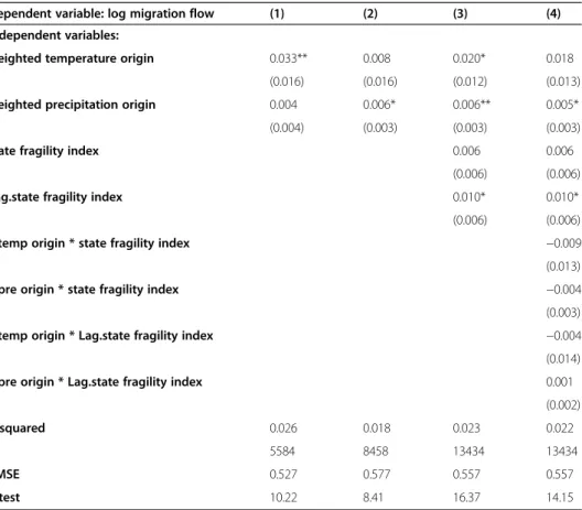
(10) Backhaus et al. IZA Journal of Migration (2015) 4:3. Page 10 of 15. dependence, we split our sample by classifying a sending country as agriculturallydependent if the share of agricultural land in its total land area exceeds 50%, which applies to 53 of the 142 countries of origin under consideration. Column 1 of Table 4 reports that for the agriculturally-dependent countries, the coefficient of the temperature changes increases by 1.4 percentage points compared to the pooled sample and is now significant at the 5% level, while changes in precipitation no longer have a significant effect. The results for the less agriculturallydependent countries presented in column 2 tend towards the opposite direction, as only the coefficient for precipitation changes remains significant and slightly increases in magnitude. These findings are unaltered when raising the cutoff share to 60%. Furthermore, they are consistent with the baseline results of a recent contribution by Cai et al. (2014) which explores this potential channel in more depth. Next, we investigate a potential three-way link between climate change, a sending country’s internal institutional and conflict environment, and emigration. An elaborate presentation of the arguments connecting these three factors can be found in Reuveny (2007). In short, we follow the notion that climate change may have more severe. Table 4 Explorations of potential channels between migration and climate change Dependent variable: log migration flow. (1). (2). (3). (4). 0.033**. 0.008. 0.020*. 0.018. (0.016). (0.016). (0.012). (0.013). 0.004. 0.006*. 0.006**. 0.005*. (0.004). (0.003). (0.003). (0.003). 0.006. 0.006. (0.006). (0.006). 0.010*. 0.010*. Independent variables: weighted temperature origin. weighted precipitation origin. state fragility index. Lag.state fragility index. (0.006). (0.006) −0.009. wtemp origin * state fragility index. (0.013) −0.004. wpre origin * state fragility index. (0.003) −0.004. wtemp origin * Lag.state fragility index. (0.014) wpre origin * Lag.state fragility index. 0.001 (0.002). R-squared. 0.026. 0.018. 0.023. 0.022. N. 5584. 8458. 13434. 13434. RMSE. 0.527. 0.577. 0.557. 0.557. F-test. 10.22. 8.41. 16.37. 14.15. Note: ***, **, * denote significance levels at one, five and ten percent, respectively. Robust standard errors are reported in parentheses. Controls and year dummies are included. Column (1) uses only countries of origin which exhibit an average share of agricultural land in their total land mass above 50%. Column (2) uses only countries of origin which exhibit an average share of agricultural land in their total land mass below or equal to 50%. Column (3) estimates the model in first differences, adding the state fragility index and its first lag. Column (4) estimates the model in first differences, adding the state fragility index, its first lag, and interactions of the two with the climate variables..

(11) Backhaus et al. IZA Journal of Migration (2015) 4:3. effects on instable and conflict-stricken countries as these countries are less capable of managing it, which in turn causes more emigration. Our proxy measure for these internal conflicts in the countries of origin is the State Fragility Index (SFI), developed by the Center for Systemic Peace (2014), which ranges from 0 to 25. The SFI is composed of two other indices, which in turn consist of indicators of a state’s economic, political, social and security effectiveness and legitimacy. Column 3 of Table 4 contains the results from adding the SFI and its first lag to specification (1). The weakly significant effect of the first lag implies that an increase in the past SFI by one unit, which corresponds to an increase in fragility, is associated with a 1% increase in bilateral migration flows. Column 4 investigates the suspected mechanism between climate change, fragility and emigration by interacting the climate variables with the SFI and its first lag. The coefficient for temperature is now insignificant, while the direct effects of the SFI and its lag remain unchanged. However, none of the interaction terms exhibit a significant coefficient, which indicates no differential impact of climatic variations conditional on a sending country’s internal stability.. 5. Conclusion This paper documents a robust relationship between climate change and migration flows. In particular, increases in temperature and precipitation in a sending country are shown to be associated with increases in migration flows to the respective destination country. Our preferred specification suggests that the effect is moderate, especially in relation to the actual climatic variations in our sample: a one degree Celsius increase in temperature is associated with a 1.9 percent increase in bilateral migration flows. An additional millimeter of precipitation is associated with an increase in migration by 0.5 percent. This finding is robust to a range of specifications, which also reveals the perhaps unanticipated importance of climatic variations for emigration from European countries. A preliminary examination of potential channels suggests that the reaction of migration due to temperature changes may in particular be driven by a sending country’s agricultural dependence. We want to point out several avenues for future research. First, it would be interesting to analyze variations in migration over time periods more extensive than 1995– 2006. Second, it might be worthwhile to disentangle the relative contributions of abrupt versus gradual changes in climate. Climate catastrophes are the focus of most of the existing literature, whereas the current study emphasizes gradual climate change. Third, we want to point out that the current results are based on data of international migration to OECD countries. Therefore, they do not take into account that emigration as a reaction to climate change may also manifest itself in a potential surge in the flows of asylum seekers or undocumented migrants. Further, neither migration between the non-OECD countries nor internal migration within the respective sending countries are considered here, but these might be of high importance. Data availability poses the main limitation for research in these directions, but narrowing the scope of analysis to specific regions or even countries and exploiting finer spatial variation in climate could deliver informative results.. Page 11 of 15.

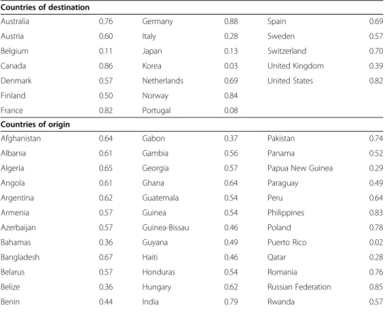
(12) Backhaus et al. IZA Journal of Migration (2015) 4:3. Page 12 of 15. Appendix This appendix contains additional figures (Figure 3) and tables (Tables 5 and 6) that supplement the main analysis in the paper.. Figure 3 Total immigrant flow by destination country.. Table 5 List of countries and share of non-missing migration observations Countries of destination Australia. 0.76. Germany. 0.88. Spain. 0.69. Austria. 0.60. Italy. 0.28. Sweden. 0.57. Belgium. 0.11. Japan. 0.13. Switzerland. 0.70. Canada. 0.86. Korea. 0.03. United Kingdom. 0.39. Denmark. 0.57. Netherlands. 0.69. United States. 0.82. Finland. 0.50. Norway. 0.84. France. 0.82. Portugal. 0.08. Afghanistan. 0.64. Gabon. 0.37. Pakistan. 0.74. Albania. 0.61. Gambia. 0.56. Panama. 0.52. Algeria. 0.65. Georgia. 0.57. Papua New Guinea. 0.29. Countries of origin. Angola. 0.61. Ghana. 0.64. Paraguay. 0.49. Argentina. 0.62. Guatemala. 0.54. Peru. 0.64. Armenia. 0.57. Guinea. 0.54. Philippines. 0.83. Azerbaijan. 0.57. Guinea-Bissau. 0.46. Poland. 0.78. Bahamas. 0.36. Guyana. 0.49. Puerto Rico. 0.02. Bangladesh. 0.67. Haiti. 0.46. Qatar. 0.28. Belarus. 0.57. Honduras. 0.54. Romania. 0.76. Belize. 0.36. Hungary. 0.62. Russian Federation. 0.85. Benin. 0.44. India. 0.79. Rwanda. 0.57.

(13) Backhaus et al. IZA Journal of Migration (2015) 4:3. Page 13 of 15. Table 5 List of countries and share of non-missing migration observations (Continued) Bhutan. 0.40. Indonesia. 0.69. Samoa. 0.20. Bolivia. 0.57. Iran. 0.70. Sao Tome&Principe. 0.22. Bosnia&Herzegovina. 0.69. Iraq. 0.67. Saudi Arabia. 0.52. Botswana. 0.46. Jamaica. 0.60. Senegal. 0.60. Brazil. 0.80. Jordan. 0.60. Sierra Leone. 0.54. Brunei Darussalam. 0.30. Kazakhstan. 0.57. Slovenia. 0.57. Bulgaria. 0.68. Kenya. 0.60. Solomon Islands. 0.11. Burkina Faso. 0.48. Kuwait. 0.43. Somalia. 0.68. Burundi. 0.53. Kyrgyzstan. 0.53. South Africa. 0.59. Cambodia. 0.55. Laos. 0.51. Sri Lanka. 0.68. Cameroon. 0.61. Latvia. 0.59. Sudan. 0.57. Cape Verde. 0.46. Lebanon. 0.66. Suriname. 0.37. Central African Rep.. 0.32. Lesotho. 0.31. Swaziland. 0.37. Chad. 0.36. Liberia. 0.54. Syria. 0.63. Chile. 0.60. Libya. 0.56. Tajikistan. 0.47. China. 0.86. Lithuania. 0.60. Tanzania. 0.59. Colombia. 0.63. Macedonia FYR. 0.56. Thailand. 0.82. Comoros. 0.20. Madagascar. 0.50. Timor-Leste. 0.08. Congo, Dem. Rep.. 0.55. Malawi. 0.50. Togo. 0.54. Congo, Rep.. 0.50. Malaysia. 0.61. Trinidad and Tobago. 0.57. Costa Rica. 0.52. Mali. 0.46. Tunisia. 0.66. Côte d’Ivoire. 0.58. Mauritania. 0.46. Turkey. 0.79. Croatia. 0.64. Mauritius. 0.59. Turkmenistan. 0.43. Cuba. 0.56. Mexico. 0.63. Uganda. 0.57. Cyprus. 0.57. Moldova. 0.61. Ukraine. 0.69. Czech Republic. 0.61. Mongolia. 0.54. United Arab Emirates. 0.44. Djibouti. 0.43. Morocco. 0.70. Uruguay. 0.52. Dominican Republic. 0.58. Mozambique. 0.55. Uzbekistan. 0.57. Ecuador. 0.62. Myanmar. 0.51. Vanuatu. 0.14. Egypt. 0.64. Namibia. 0.50. Venezuela. 0.68. El Salvador. 0.53. Nepal. 0.57. Viet Nam. 0.79. Equatorial Guinea. 0.22. New Zealand. 0.62. Yemen. 0.50. Eritrea. 0.54. Nicaragua. 0.54. Zambia. 0.57. Estonia. 0.60. Niger. 0.49. Zimbabwe. 0.56. Ethiopia. 0.64. Nigeria. 0.64. Fiji. 0.45. Oman. 0.45.

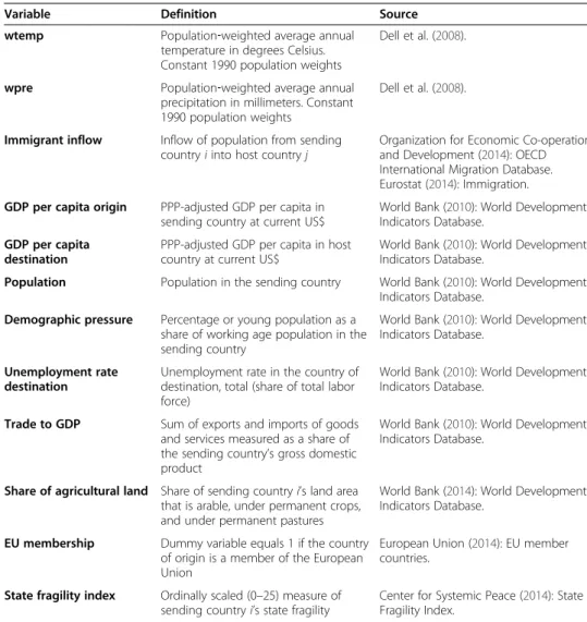
(14) Backhaus et al. IZA Journal of Migration (2015) 4:3. Page 14 of 15. Table 6 List of variables and sources Variable. Definition. Source. wtemp. Population‐weighted average annual temperature in degrees Celsius. Constant 1990 population weights. Dell et al. (2008).. wpre. Population‐weighted average annual precipitation in millimeters. Constant 1990 population weights. Dell et al. (2008).. Immigrant inflow. Inflow of population from sending country i into host country j. Organization for Economic Co-operation and Development (2014): OECD International Migration Database. Eurostat (2014): Immigration.. GDP per capita origin. PPP-adjusted GDP per capita in sending country at current US$. World Bank (2010): World Development Indicators Database.. GDP per capita destination. PPP-adjusted GDP per capita in host country at current US$. World Bank (2010): World Development Indicators Database.. Population. Population in the sending country. World Bank (2010): World Development Indicators Database.. Demographic pressure. Percentage or young population as a World Bank (2010): World Development share of working age population in the Indicators Database. sending country. Unemployment rate destination. Unemployment rate in the country of destination, total (share of total labor force). World Bank (2010): World Development Indicators Database.. Trade to GDP. Sum of exports and imports of goods and services measured as a share of the sending country’s gross domestic product. World Bank (2010): World Development Indicators Database.. Share of agricultural land Share of sending country i’s land area that is arable, under permanent crops, and under permanent pastures. World Bank (2014): World Development Indicators Database.. EU membership. Dummy variable equals 1 if the country European Union (2014): EU member of origin is a member of the European countries. Union. State fragility index. Ordinally scaled (0–25) measure of sending country i’s state fragility. Center for Systemic Peace (2014): State Fragility Index.. Competing interests The IZA Journal of Migration is committed to the IZA Guiding Principles of Research Integrity. The authors declare that they have observed these principles. Acknowledgements The authors would like to thank the editor and one referee for their helpful comments and suggestions. Further, the authors acknowledge the support and collaboration of Project ECO2010-15863 funded by the Spanish Ministry of Innovation and Science and the Entdecken Project funded by the German Ministry of Education and Research (Bundesministerium für Bildung und Forschung). We also would like to thank the participants of the III Entdecken workshop held in Goettingen for their helpful comments and suggestions. Responsible editor: Amelie F Constant. Author details 1 University of Munich, Chair for Population Economics, Schackstr. 4/IV, 80539 München, Germany. 2University of Goettingen, Platz der Göttinger Sieben 3, 37073 Göttingen, Germany. 3Universidad Jaume I, Castelló de la Plana, Spain. 4 Department of Economics, Simon Fraser University, 8888 University Drive, Burnaby, BC V5A 1S6, Canada. Received: 31 March 2014 Accepted: 2 December 2014. References Afifi T, Warner K (2008) “The Impact of Environmental Degradation on Migration Flows across Countries”, Working Paper No.5/2008. UNU-EHS, Bonn Beine M, Parsons C (2013) “Climatic Factors as Determinants of International Migration”, CREA Discussion Paper Series 12–01. CREA, Luxembourg.

(15) Backhaus et al. IZA Journal of Migration (2015) 4:3. Page 15 of 15. Belasen AR, Polachek SW (2013) Natural disasters and migration. In: Constant AF, Zimmermann KF (eds) The International Handbook on the Economics of Migration. Edward Elgar Publishing, Cheltenham, UK, pp 309–330, Chapter 17 Cai R, Feng S, Pytliková M, Oppenheimer M (2014) “Climate Variability and International Migration: the Importance of the Agricultural Linkage”, IZA Discussion Paper No. 8183. IZA, Bonn Cole BR, Marshall MG (2014) State Fragility Index and Matrix. Center for Systemic Peace, Vienna USA Dell M, Jones BF, Olken BA (2008) “Climate Change and Economic Growth: Evidence from the Last Half Century”, National Bureau of Economic Research Working Paper 14131. NBER, Cambridge Dell M, Jones BF, Olken BA (2014) What do we learn from the weather? The new climate-economy literature. J Econ Lit 52(3):740–98 Eurostat (2014) Immigration by Five Year Age Group, Sex and Citizenship. European Commission, Eurostat, Luxemburg IPCC (2007) Climate Change 2007: Synthesis Report. In: Core Writing Team, Pachauri RK, Reisinger A (eds) Contribution of Working Groups I, II and III to the Fourth Assessment Report of the Intergovernmental Panel on Climate Change. IPCC, Geneva Mayda A (2010) International migration: a panel data analysis of the determinants of bilateral flows. J Popul Econ 23:1249–1274 Naudé W (2009) Natural disasters and international migration from Sub-Saharan Africa. Migrat Lett 6(2):165–176 OECD (2014) International Migration Database. OECD, Paris Reuveny R (2007) Climate change-induced migration and violent conflict. Polit Geogr 26(6):656–673 Reuveny R, Moore WH (2009) Does environmental degradation influence migration? Emigration to developed countries in the late 1980s and early 1990s. Soc Sci Q 90(3):461–479 Ruyssen I, Everaert G, Rayp G (2014) Determinants and dynamics of migration to OECD countries in a threedimensional panel framework. Empir Econ 46:175–197 Warner K, Stal M, Dun O, Afifi T (2009) Researching environmental change and migration: evaluation of EACH-FOR methodology and application in 23 case studies worldwide. In: Laczko F, Aghazarm C (eds) Migration, Environment and Climate Change: Assessing the Evidence. IOM, Geneva, pp 197–244 World Bank (2010) World Development Indicators 2010. World Bank, Washington D.C World Bank (2014) World Development Indicators 2014. World Bank, Washington D.C. Submit your manuscript to a journal and beneﬁt from: 7 Convenient online submission 7 Rigorous peer review 7 Immediate publication on acceptance 7 Open access: articles freely available online 7 High visibility within the ﬁeld 7 Retaining the copyright to your article. Submit your next manuscript at 7 springeropen.com.

(16)