Principles of Revenue Management and their applications

UNIVERSIDAD DE VALLADOLID

ESCUELA DE INGENIERIAS INDUSTRIALES

Grado en Ingeniería en Organización Industrial

Principles of Revenue Management and their

applications

Autor:

Oliveri Martínez-Pardo, Gonzalo

Responsable de Intercambio en la UVa

Gento Municio, Ángel Manuel

Universidad de destino

1

Valladolid, 08/2017.

TFG REALIZADO EN PROGRAMA DE INTERCAMBIO

TÍTULO:

Principles of Revenue-Management and their applications

ALUMNO:

Gonzalo Oliveri Martínez-Pardo

FECHA:

24/07/2017

3

BACHELOR THESIS

“Principles of Revenue-Management and

their Applications”

AUTHOR:

GONZALO OLIVERI MARTÍNEZ-PARDO

5

Eidesstattliche Erklärung / Affidavit

Ich versichere, die Arbeit selbständig verfasst zu haben und keine anderen Quellen und Hilfsmittel benutzt zu haben. Alle Stellen, die wörtlich oder sinngemäß aus Veröffentlichungen entnommen sind, habe ich als solche kenntlich gemacht.

I hereby declare that this project work has been written only by the undersigned and without any assistance from third parties.

Furthermore, I confirm that no sources have been used in the preparation of this work other than those indicated in the thesis itself.

6

Index

1. INTRODUCTION ... 11

1.1. CONCEPTUAL FRAMEWORK OF REVENUE MANAGEMENT ... 11

1.1.1. Management decisions ... 11

1.1.2. Properties that encourage the application of Revenue Management ... 12

1.1.3. The Revenue Management process ... 14

1.2. HISTORY ... 15

1.3. REVENUE MANAGEMENT IN 21th CENTURY ... 19

1.3.1. Revenue Management in the Industry ... 19

1.3.2. How to conduct Revenue Management in a company ... 20

1.3.3. Important factors in Revenue Management ... 20

2. KEY IDEAS ... 22

2.1. QUANTITY-BASED METHOD ... 22

2.1.1. Types of controls ... 23

2.1.2. Overbooking ... 26

2.2. PRICE-BASED METHOD ... 28

2.2.1. Factors must be considered in dynamic-pricing models ... 28

2.2.2. Customers segmentation in RM pricing ... 29

2.2.3. How to set prices ... 31

2.3. PRICE-BASED VS QUANTITY-BASED ... 32

3. MODELS ... 34

3.1. CAPACITY CONTROL MODELS ... 34

3.1.1. n-Class model ... 34

3.1.2. Heuristic models ... 39

3.2. STATIC OVERBOOKING MODEL: THE BINOMIAL MODEL ... 45

3.2.1. Overbooking based on Service-Level Criteria ... 47

3.2.2. Overbooking based on Economic criteria ... 48

3.3. DYNAMIC PRICING MODEL ... 50

3.3.1. Model´s enunciate ... 50

3.3.2. Solving the problem ... 51

3.3.3. Example ... 52

7

4.6. Online travel portals ... 61

4.7. Restaurants ... 62

4.8. Passenger railways ... 63

4.9. Theatres and Sport events ... 63

4.10. Freight ... 64

4.11. Tour operators... 64

4.12. Programs used in Hotel industry ... 65

4.12.1. STR... 65

4.12.2. IDeaS ... 66

4.12.3. HotelsDot ... 66

4.12.4. Modern Revenue... 66

5. CONCLUSIONS ... 67

6. APPENDIX: ... 68

6.1. Appendix 1: Table of normal distribution ... 68

6.2. Appendix 2: Graphic of c.d.f. distribution ... 69

8

List of tables

Table 1: Management decisions (contents from [2]) ... 11

Table 2: Properties that encourage the application of RM (contents from [3] p.4-7) .... 13

Table 3: Distribution of the full rate demand [35] ... 17

Table 4: Important factors in dynamic pricing models (contents from [2] p.182-187) ... 29

Table 5: Matrix of segmentation [34] ... 30

Table 6: Different kind of rate fences (Information from [3] p.15-16) ... 31

Table 7: Prices and demand data for each class ... 37

Table 8: Results of the example 3.1.1.2. ... 39

Table 9: Demand data for each class [2] ... 41

Table 10: Results of heuristic models and comparison with the optimal policy [2] ... 45

Table 11: Expected revenues obtained for different capacities and comparison with the optimal [2] ... 45

Table 12: Binomial approximation overbooking probabilities [2] ... 48

Table 13: Results of the first numerical example 3.3.3. ... 55

Table 14: Results of the second numerical example 3.3.3. ... 56

Table 15: How hotels satisfy Revenue Management favourable conditions ... 57

Table 16: How Rental car companies satisfy R M favourable conditions ... 58

9

Table 18: How electricity companies satisfy R M favourable conditions ... 61

Table 19: How online travel portals satisfy R M favourable conditions ... 62

Table 20: How restaurants satisfy R M favourable conditions ... 62

Table 21: How satisfy Theatres and sport events RM conditions ... 63

10

List of figures

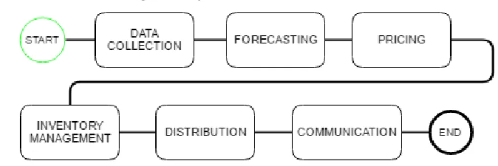
Figure 1: Revenue Management process (By my own) ... 14

Figure 2: Important factors in the future (Graphic from [6] p.23) ... 20

Figure 3: Booking limits (bi) and protection levels example (yi) [2] ... 23

Figure 4: Booking limits (b), protection levels (y) and bid prices (π(x)) relation [2]... 25

Figure 5: Optimal protection level yi* in the model [2] ... 36

Figure 6: Overbooking limits and reservations over the time [18] ... 46

Figure 7: Table of normal distribution [24] ... 68

11

1. INTRODUCTION

The intention of this thesis is to show some ideas about the concept of Revenue Management. This thesis begins with an introduction that contents general ideas about Revenue Management. Later, it is explained in more detail some key ideas of RM and some basic models in RM. Afterward some applications in the real world and software used in RM are presented and finally there are some conclusions.

1.1. CONCEPTUAL FRAMEWORK OF REVENUE MANAGEMENT

Revenue management is defined as the collection of strategies and tactics firms use to scientifically manage demand for their perishable products and services [1].

Every seller faces several fundamental decisions. You want to sell when market conditions are most favourable; you want the right price (not so high that you put off potential customers and not so low that you lose out on profits) and you want to know how customers value your product. Businesses face these and other complex decision with the aim of maximize benefits [1].

1.1.1. Management decisions

Revenue management (RM) is concerned with the methodology and systems required to make demand management decisions. Next table (Table 1) shows the three categories of management decisions showed in Theory and Practice of Revenue

Management [2].

MANAGEMENT DECISION DECISIONS ABOUT

Structural decisions

- Which sales channel to use for selling the products or service.

- Which segmentation mechanism to use. - Which terms of trade to use.

- Which set of products to offer.

Prices decisions

- How to set prices and individual offers. - How to price over time.

- How to establish different category prices. - How to set discounts over the product lifetime.

Quantity decisions

- Whether accept or reject an offer.

- How to set the capacity to different products, segments or channels.

- When refuse a sale and sale this product later.

12 To decide which of these decisions is the most important depends on the context. Structural decisions about channels for selling and the tools for grouping products are strategic decisions that are not taken frequently. Firms also should take decisions about prices or quantity which change their ability to adjust price or quantities on a tactical level. The ability to adjust quantities may be a function of the flexibility of the supply process and the costs of real locating capacity and inventory. For example, Airlines use capacity controls as a tactic because of the fact that the different products that they sell (different ticket types sold at different times and under different terms) are all provided using the same, homogeneous capacity [1].

Revenue Management can be qualified as being either quantity-based RM or price-based RM if it uses capacity-allocation decisions or price decisions as the first tactical tool for managing demand. These two terms are explained more extensively in second chapter.

1.1.2. Properties that encourage the application of Revenue Management

13

PROPERTY EXPLANATION EXAMPLE

Relatively fixed capacity

The production is

constant, it is not able to increment the production in a brief time period

In each flight, there are a limited number of seats

If there are available seats for a flight today, these seats cannot be stored for another flight that is full.

Inventoried demand

Most industries that employ RM use

reservations to anticipate and to control the future demand by the selling of products before the

Stochastic demand Most of demand varies

over time.

Consider the demand for air travel. It varies due to season, time of day, day of week, holidays, …

High fixed costs The combination of high fixed costs and low variable costs gives more incentive to fill their unused capacity

In a flight, there are high fixed costs (plane, staff, …) and insignificant variable costs for selling an unused seat. Airlines are interested in selling all the capacity evena low price. but others are willing to pay more for a better service. Then it is necessary to make a segmentation of customers.

A student or family in holidays are willing to although he has to pay more money.

Table 2: Properties that encourage the application of RM (contents from [3] p.4-7)

14

1.1.3. The Revenue Management process

Stuart-Hill in an article [4] shows the process that most practitioners follow today involves a continuous cycle of six basic steps:

- Step 1: Data collection

The best decisions are often a mix of intuition and science. In order to understand the impact of these decisions, it is recommendable to store data and to use those to help make better decisions in the future.

Automation and decision support tools have evolved as the revenue management discipline has grown and provide business insights that humans are not able to calculate on their own. The ideal solution is when automation provides insights for the revenue management professional and the revenue management professional provides appropriate feedback within the system.

- Step 2: Forecasting

Predicting future demand based on past results is a good starting point to develop a strategy. Of course, changes in market conditions, competitive supply, capacity constraints, special events, floating holidays, weather conditions, economic climate and other external factors need some additional thought around true demand potential; but the past results provide help to make good predictions and to be prepared against the variations produced by these factors.

- Step 3: Pricing

People who unknow the scope of the discipline often think that revenue management simply consists in changing prices, or making discounts. The fact is that pricing is far more complex than this.

Basic economic theory would dictate that equilibrium pricing, where the demand curves meets the supply curve, would be optimal. Unfortunately, inventory is perishable so this approach would not utilize all the resource's potential.

- Step 4: Inventory Management

Once future demand has been forecasted and pricing strategies determined, resource allocation or inventory management comes into play. Inventory management simply means opening or restricting inventory for sale based on certain conditions as the available capacity.

15 - Step 5: Distribution

Distribution refers to how guests find and book a property. Telephone, Online Travel Agencies, Global Distribution Systems and Internet Booking Engines are all examples of distribution channels. Each one may offer a different value proposition, but each one requires that a revenue management professional think through how to best leverage the potential that each one represents.

- Step 6: Communication

Communication is crucial because Revenue Management requires that a firm must continually re-evaluate their prices, products, and processes in order to maximize revenue. In a dynamic market, an effective Revenue Management System constantly re-evaluates the variables involved in order to move dynamically with the market. Then communication is causal because the information is constantly varying.

Of course, once a strategy has been implemented the process begins again with Step 1 - tracking. This process is one of continuous improvement; however, some elements of experimentation will depend of the probability. Then, some actions will have a positive impact and others won't. The secret is when there is a fail, find it quickly and ensure learning is documented.

In few words, Revenue Management’s basis is “to sell the correct product to the right

client at the right price in the right moment”. But to understand in a better way what is

Revenue Management it should be recommendable to take a look at its origins.

1.2. HISTORY

The interest in revenue management practices started during the 70s with the researches of Littlewood (1972) on overbooking in airlines. These researches have as a result, the rule known as Littlewood’s rule.

Littlewood proposed that when a product has two different prices, the product must be sold at the lower price until the probability of selling at the higher-price is higher than the relation between the two prices.

- LITTLEWOOD RULE:

Littlewood considered a flight with two different rates, 𝒑𝟏 and 𝒑𝟐 (with 𝒑𝟏 > 𝒑𝟐),

and demand of 𝒑𝟏 is sold after the demand of 𝒑𝟐. Littlewood proposed that the

16

𝑷(𝒑𝟏) >

𝒑𝟐

𝒑𝟏

{

𝑃(𝑝1) ∶ 𝑃𝑟𝑜𝑏𝑎𝑏𝑖𝑙𝑖𝑡𝑦 𝑜𝑓 𝑠𝑒𝑙𝑙𝑖𝑛𝑔 𝑝𝑟𝑜𝑑𝑢𝑐𝑡 𝑎𝑡 𝑝𝑟𝑖𝑐𝑒 1

𝑝2: 𝑙𝑜𝑤𝑒𝑟 − 𝑝𝑟𝑖𝑐𝑒

𝑝1: ℎ𝑖𝑔ℎ𝑒𝑟 − 𝑝𝑟𝑖𝑐𝑒

The solution can be obtained from the relationship marginal revenue/loss. To get the solution, it is supposed there are 𝒏 vacant units and one class 2 client wants to buy a seat. In case of the airline regret the purchase, it will be sold𝒏 units at

𝒑𝟏 only in the case if demand of class 1 is higher or equal than

𝒏(𝑫𝟏 ≥ 𝒏). As a result, marginal revenue of the booking of this seat for class 1

will be 𝒑𝟏∗ 𝑷(𝑫𝟏 ≥ 𝒏). Finally, it is logic to accept class 2 clients always that 𝒑𝟐

would be equal or higher than this marginal revenue 𝒑𝟐 ≥ 𝒑𝟏∗ 𝑷(𝑫𝟏 ≥ 𝒏).

As 𝒏 is decreasing, after the moment that 𝒑𝟏∗ 𝑷(𝑫𝟏 ≥ 𝒏) is higher than 𝒑𝟐, it will

be always higher, then exists an optimal protection level 𝒚𝟏∗ such that we accept

class 2 until the moment that available capacity is equal or less than 𝒚𝟏∗. Then,

𝒚𝟏∗ satisfies:

𝒑𝟐< 𝒑𝟏∗ 𝑷(𝑫𝟏≥ 𝒚𝟏∗) 𝑎𝑛𝑑 𝒑𝟐 ≥ 𝒑𝟏∗ 𝑷(𝑫𝟏 ≥ 𝒚𝟏∗ + 𝟏)

If the demand is modelled by the continuous distribution 𝑭𝟏(𝒙), Then, we have:

𝒑𝟐= 𝒑𝟏∗ 𝑷(𝑫𝟏≥ 𝒚𝟏∗)equivalently, 𝒚𝟏∗ = 𝑭𝟏−𝟏(𝟏 − 𝒑𝟐 𝒑𝟏) that is known as Littlewood’s rule.

Now, it is shown a little example [35] to understand better how it works:

An airline offers two different rates for the same flight: full rate (𝒑𝟏= 𝟒𝟏𝟖€) and

Economic rate (𝒑𝟐= 𝟐𝟏𝟖€). The capacity is 𝑪 = 𝟐𝟑𝟎 and the demand for the full

17

Table 3: Distribution of the full rate demand [35]

Now, it is determined the number of Full seats and the limit of Economic seats by the Littlewood´s rule. To get it, it is determined the highest value of Q that satisfy:

𝒑𝟏∗ 𝑷(𝑫𝟏≥ 𝑸) + 𝟎 ∗ 𝑷(𝑫𝟏< 𝑸) ≥ 𝒑𝟐

Now, it is looked for the value that satisfy it:

For 𝑸 = 𝟒𝟓, 𝑷(𝑫𝟏 ≤ 𝑸) = 𝟎, 𝟒𝟗 and 𝑷(𝑫𝟏= 𝑸) = 𝟎, 𝟎𝟕

Then, 𝑷(𝑫𝟏< 𝑸) = 𝑷(𝑫𝟏≤ 𝑸) − 𝑷(𝑫𝟏= 𝑸) = 𝟎, 𝟒𝟗 − 𝟎, 𝟎𝟕 = 𝟎, 𝟒𝟐 < 𝟎, 𝟓𝟎𝟒

For 𝑸 = 𝟒𝟔, 𝑷(𝑫𝟏 ≤ 𝑸) = 𝟎, 𝟓𝟏 and 𝑷(𝑫𝟏= 𝑸) = 𝟎, 𝟎𝟐

18 For 𝑸 = 𝟒𝟕, 𝑷(𝑫𝟏 ≤ 𝑸) = 𝟎, 𝟓𝟒 and 𝑷(𝑫𝟏= 𝑸) = 𝟎, 𝟎𝟑

Then, 𝑷(𝑫𝟏< 𝑸) = 𝑷(𝑫𝟏≤ 𝑸) − 𝑷(𝑫𝟏= 𝑸) = 𝟎, 𝟓𝟒 − 𝟎, 𝟎𝟑 = 𝟎, 𝟓𝟏 > 𝟎, 𝟓𝟎𝟒

The highest value of Q that satisfy the Littlewood’s rule is Q=46; that is the number of Full seats. As a consequence, 230-46=184; are the maximum number of seats accepted for the Economic class.

During the first years of Revenue Management was the basis of the algorithms used by

the automatized systems of Revenue Management.

October of 1978 was a crucial moment during the beginnings of Revenue Management

because it was the year when the airline deregulation was signed in USA. This supposed

the end of the monopoly protection of the biggest airlines in the country and the entrance

of new competitors and the free airfares.

The entrance of new companies supposed many problems for the big six that are the

companies which had been protected by the government from 1937 until 1977 (American

Airlines, Delta Air Lines, USAir (now belongs to AA), Continental Airlines (acquired by

United Airlines), United Airlines and Eastern Airlines (dissolved in 1991)), in fact some

of them disappeared and the others offered discounted rates. One of these new

companies was People Express, this low-cost company appeared in 1981 and gain much

importance and it was a big threat for the big six.

The answer of American Airlines came in December of 1985 with discounted rates (up

to 80% lower than the usual rate) called ‘Ultimate Super-Saver fares’(uss). The

difference with other discounted rates was DINAMO (Dynamic Inventory Optimization

and Maintenance Optimizer) that represents the first large-scale RM system

development in the industry.

DINAMO is the automatized system developed by American Airlines to include

Littlewood´s rule in their decisions and reduced the proportion of flights requiring analyst

review from 100 percent to approximately 5 percent [5]. DINAMO calculated dynamically

the probability of sale the last seat in the highest rate using the Littlewood´s rule. It optimized the quantity of seats that were offered with ‘ultimate supersaver’ rate. Due to

the success of DINAMO People Express broke down and was sold to Continental Airlines

a year later and the revenues of American Airlines grew up $1.4 billion during the next

three years.

Donald Burr, CEO of People Express, summarized the reasons behind the company’s

failure: “We were a vibrant, profitable company from 1981 to 1985, and then we tipped

19

changed was American’s ability to do widespread Yield Management in every one of our markets. ...We did a lot of things right. But we didn’t get our hands around Yield Management and automation issues. ... [If I were to do it again,] the number one priority on my list every day would be to see that my people got the best information technology tools. In my view, that’s what drives airline revenues today more than any other factor— more than service, more than planes, more than routes.”

These is the moment when the airline industry provided a concrete example of the great impact that the revenue management can have on the operations of a company. At this stage, however, much of the work was about capacity management and overbooking and only a little about dynamic pricing policies. In these original models, prices were assumed to be fixed and managers only decide about how many seats sell in each class.

During the 1990s the increasing interest in revenue management made evident the different applications that can be considered. Models became industry specific with a higher complexity. Moreover, is during this decade when prices policies became an important component of the revenue management activities.

As we said, the airline industry leaded the use of revenue management techniques in terms of capacity/seat control and dynamic pricing.

1.3. REVENUE MANAGEMENT IN 21th CENTURY

What is special about revenue management is not which decisions are made but rather how are decisions made to get the aim of increasing benefits in every budget that you can use; then, what develop is the tools that Revenue Management to get the goal [17]. The new about RM is the method of decision making, that is driven by two complementary points. First, the scientific advances allow computing optimal real-time solutions to complex decision problems. The other point resides in that the advances in information technology provide the capability to automate transactions, store and implement the data and manage detailed demand-management decisions [17].

1.3.1. Revenue Management in the Industry

There are other examples besides airlines of the success of Revenue management, as the case of hotels. First in hotels, RM only was applied to rent bedrooms. But nowadays it is used in every part in the hotel (restaurant, parking, golf, spa, …) in response to the increments caused by the application of RM in bedrooms management. As Kimes said “each squared meter in the hotel is susceptible of generate revenues” [6]. This high grow has taken place in less than 20 years.

20 around Internet, software programs and big-data; that permit to work easier and more efficiently than some years ago. In fact, until 1990s Revenue Management only was useful as philosophy to manage in airline industry but now it has reached other sectors [17].

Some of the industries that use Revenue Management are explained in more detail in chapter 4.

1.3.2. How to conduct Revenue Management in a company

The future of how to manage the RM in a company is already uncertain. In the case of hotel chains, Kimes´ investigation [6] (p.5) shows two tendencies of how to solve the management.

First tendency is thought that in the future, Revenue Management department will be an independent department which combines Marketing and Business because the aim is to sell in the most efficient way as possible but without damaging the image of the product.

The second tendency talks about a future where the tendency in management in hotel chains will be the centralization or a hybrid model that consists in that centrals transmits a general view and hotels offer a concrete view of each case. For example, the group NH hotels has the management centralized for all hotels but there are some concrete management decisions those are taken by each hotel.

1.3.3. Important factors in Revenue Management

In the same investigation [6], Kimes conducted a survey among professionals in the field. Results shown that technology is the most important RM influencing factor, as it is showed in figure 2:

21 The graphic shows the future influence of the different RM influencing factors among the respondents. Consumer behaviour, Competition, Internet, Market segmentation and Economy are factors that influence in products’ prices. But Technology is the most important one because is the tool to take advantage respect the influence of the other factors.

Although these results come from a survey among professionals in Revenue Management, they could be the same for other general consumer choice situations.

As we all know now we are living a technologic-boom caused by the constant development. Technology is growing exponentially and Revenue Management take advantage of that because tools used to take decisions are being developed at the same time.

22

2. KEY IDEAS

As it is shown in the Introduction, in Revenue Management we can distinguish two methods to work. The first, and older, is the Quantity-based method. This method has as main idea the control of the quantity of products are sold with each price. In the field of airlines, it would be the method that help to make decisions on how seats must be sold in each flight at each rate to maximize profits.

The second method is the Price-based Revenue Management. This method works to control and to adjust the prices to maximize their benefits.

2.1. QUANTITY-BASED METHOD

Quantity-based method has as main idea the control of the quantity of products we sold with each price. In the field of airlines, it would be the method that help to make decisions on how seats we must sell in each flight at each rate to maximize profits [2].

To explain it better, it will be used an example. It is the case of a single leg flight or a night in a hotel. For trying to sell every seats or rooms, companies offer two different rates the business-rate (higher-price) and the tourist-rate (more economic price). The question is now how many products must be sold at each price for the optimization of benefits. The problem is the customer heterogeneity that consists in that different people rate the same product at a different value. Then, if you offer too many business-rate products, not all the products will be sold. In the other case if you don´t offer enough business-rate products, you will sell some tourist-rate products that could have been sold more expensively.

Quantity-Based RM use some tools to give an answer of the question and to offer some optimized solutions in real-time that helps in the decisions about how many products offer in each fare.

The central problem is how to assign optimally the capacity of resources to the different customers. This assignation must be done dynamically as demand materializes and with considerable uncertainty about the quantity or composition of future demand. To make this assignation widely it is crucial to make a good segmentation of the demand in function of their willingness to pay different rates.

There are some different ways to make a segmentation but it is necessarily to consider two aspects: first, the distribution channel used by customers to make their bookings; and second, the price, that is the tool to segment the customers offering different rates in function of extra-services, purchase channel, … There are some requirements to know that the segmentation is correct [33]:

- Homogeneity in the segment. - Heterogeneity between segments. - Stability of segments.

23 Now the different controls used to control the future demand are shown.

2.1.1. Types of controls

To work efficiently, companies must realise some controls. In the travel Industry, the availability of bookings is controlled every time because the data saved and implemented every moment and the system works dynamically. These controls [17] are:

2.1.1.1.

Booking limits:

These limits are responsible of restricting the amount of capacity that can be sold to each class at a given point in time. For example, if the booking limit is 24 on class 1, it indicates that the most amount of capacity that can be sold to customers in class 1 is 24.

Booking classes can be partitioned or nested. The partitioned booking limit divides the capacity in separate blocks for each class. The sum of booking limits of all the classes must be equal than the whole capacity.

In the case of a flight, with three different classes and a whole capacity of 30 passengers we have these booking limits: 12(class 1), 10 (class 2), 8 (class 3). The limits can be changed but the sum of all must be 30.

Then when, we have sold 12 of class 1, class 1 would be closed. This could be undesirable when class 1 has higher revenues than the other classes and the amount allocated to class 1 are sold out.

Nested booking limit works in a different way to solve the problem with the partitioned booking limits. In this case, also there are different booking limits for each class, but the difference resides in that higher classes have access to all the capacity of the lower classes. For the case we saw before, the nested booking limits would be b1=30 for the set 1 (because class 1 is the highest then it has access to the units of the other two classes), b2=18 for set 2 (includes the 10 units for class 2 and the 8 for class 3) and b3=8 for set 3 (because it is the third lower class, it only has access its own units). It is shown in the Figure 3.

Nested booking limits are used by almost every reservations system because they allow to solve the problem of capacity being simultaneously unavailable for a high class yet available for lower classes.

24

2.1.1.2.

Protection levels

Protection levels are used to reserve an amount of capacity for a class or set of classes. As in booking limits, protection levels can also be nested or partitioned.

A partitioned protection level is essentiality the same than a partitioned booking limit. A booking limit of 10 on class 2 sales is equivalent to a protection level of 10 units of capacity for class 2.

Nested protection levels are again defined for sets of classes but in reverse order. For nested booking limits, each set of classes includes a class and the lower class (in the example b1 includes all classes, b2 includes class 2 and 3 and b3 only includes class 3).

Instead for nested protection levels each set of classes includes its class and higher classes. Then in the example we would have these protection levels: y1=12 for set 1(only includes class 1 because is the highest), y2=22 for set 2 (includes class 2 and higher, class 1) and y3=30 (includes all classes because third class is the lowest). Thus, we have 12 units reserved for class 1, 22 for classes 1 and 2 and 30 for every class.

Then, if 12 units of class 1 are sold you can continue selling because there are reserved 30 seats for the three classes then class 1 has already access. In the other hand, if 8 units of class 3 are sold, you can´t sell more class 3 because all the other units are reserved for classes 1 and 2.

In the figure 3 (page before), we can see that the booking limit for class (set) j is simply the capacity (C) minus the protection level for set j-1.

𝒃𝒋= 𝑪 − 𝒚𝒋−𝟏, 𝒋 = 𝟐, … , 𝒏

Besides b1 = yn = C because the booking limit for highest class is all the capacity and

the protection level for all classes combined (the lowest, that includes every class higher) is al capacity too.

2.1.1.3.

Standard/ Theft Nesting:

There are two different process for using nested booking limits or nested protection levels. The standard process starts with C units of capacity. It is accepted a booking for class j when there is capacity available and the total request accepted for class j and lower (j, j+1, …, n) is less than the booking limit bj. (also, the current capacity

available is more than the protection level yj−1 for classes higher than j).

In theft nesting process, a booking in class j don´t reduce the units for class j, and takes the allocation of the lower classes. This is the same than keeping yj units of

25 higher, and to reduce the allocation for classes j+1, j+2, ..., n. In contrast, under standard nesting, when we accept a request from class j we only reduce by one the capacity we protect for future demand from class j and higher. In the example of the figure 3, if we would accept a request for class 1, y1 would continue valuing 12; but

y2 and y3 would be reduced: y2=21 and y3=29.

2.1.1.4.

Bid prices:

What makes bid-price controls special from booking limits and protection levels is that bide-price controls are based in the revenues from each sale, rather than class-based controls. A bid-price control establishes a threshold price (which may depend on variables such as the remaining capacity or time) and request for booking is accepted if its revenue exceeds the threshold price and rejected if it is less than the threshold price.

Firstly bid-price controls look simpler than protection-level and booking-limit controls because they only need set only a single threshold value at any point in time. However, to work effectively, bid prices must be actualized after each sale and this usually needs to store a table of bid-prices values directed by the current remaining capacity, current time, or both.

The figure 4 shows how can be used bid prices to implement the same example as the other two types of control where the bid price π(x) is planned as a function of the remaining capacity x. When there are between 22 and 30 available units bid-price is lower than 50$ (all the three classes are accepted). With 13 to 22 units, bid-price is between 50$ and 75$ (only classes 1 and 2 are accepted). And when there are 12 or less units available, bid-price is over than 75$ but less than 100$ (only class 1 demand is accepted).

26 Some experts criticize Bid-price because consider it unsafe because use only a threshold price as the only control. That means that RM system sell an unlimited number of units to any class whose revenues exceed the bid-price threshold. However, this is truth only when the bid price is not actualized. As it is shown in the figure 4, if the bid-price is function of remaining capacity (bid-price is actualized after each purchase), then it works like the other two methods, closing off capacity to successively higher classes as capacity is consumed. This function is necessary because a simple static threshold is indeed a somewhat dangerous form of control.

One advantage of bid-prices controls is the ability to discriminate because it is based on revenue rather than on class. Often some customers with different willingness to pay are in a single class using an average price as the price for this class. However, if actualized revenue information can be used for each request, then a bid-price control can selectively accept only the higher revenue requests in a class, while the other controls can only accept or reject all requests of a class. But if it is not possible to observe the exact revenue at the time of reservation, then this advantage is lost.

Bid-prices don´t segment the demand in different closed class with the average price. In the example that we are using during the explanation, it is supposed that there are only seats available for class 1. If we use the other two controls, you only accept people that are willing to pay 100$ and reject the others and maybe it is not possible sell all of them. But using bid prices some customers who are willing to pay between 75$ and 100$ are accepted when this price is higher than bid-price. This fact provides the airline the opportunity of selling more seats.

It could be thought that bid-prices are controls for dynamic pricing but it is not truth because what this control vary is the minimum price that must be accepted for each available capacity to increase the revenues.

Figure 3 shown the examples that we use in the three controls. At the top, it is shown the relationship between booking limits and protection levels. At the bottom, we can see how would vary bid-prices in function of the available capacity.

2.1.2. Overbooking

Some experts [2] consider overbooking as essential activity in Revenue Management. Overbooking is distinct from the two models; indeed, overbooking is the oldest of RM practices. It is an important activity although it is not the principal strategy. The objective of overbooking is to maximize the capacity utilization of the system in the presence of cancelations and, consequently, the benefits.

As most people know, overbooking essentially consists in accepting more reservations than units you have available [11]. It is applicable when the follow characteristics [12] are fulfilled:

- Capacity is constrained and perishable and bookings are accepted for future use. - Customers can cancel or no-show.

27 Despite most of customers have bad perception of Overbooking, companies continue using it; but, why Overbooking? The reason is simple, companies that accept advance bookings with refundable sales run the risk of cancellations. Overbooking only is a strategy that firms for protecting themselves from this risk and thus it increases the utilization of capacity and maximize revenue for the firm. But it must be well implemented because it is useful only if it works well. If the Overbooking is not well implemented it only increment the costs and reduce the revenues. Thus, it is necessary to face some problems. One problem is facing the legal and regulatory implications of failing the booking contract. Companies must have operational policies and procedures used when a service must be denied.

When there are oversales, managing the compensation and the selection of customers can have a significant impact on denied-service costs and customers perception of overbooking. We next look at the main issues involved in managing oversales [2]:

- Compensation of Denied Service: Legally mandated compensations often specify a payment of monetary damage; but it is often inadequate for the customers’ perception. It is usually more effective to offer a substitute service (more quality service), because sometimes customers are not interested in an economic compensation, they only want to enjoy the service then they are usually more satisfied when they receive a more quality service than an economical compensation.

- Selection of customers: The selection of customers who will be denied also can have a significant impact in firm´s costs and in customers´ perception. From a legal standpoint, selection must not be discriminatory.

The most intuitive option for allocating a service to customers it is to do it on a first-come, first serve (FCFV). It means that customers are served when they arrive until the service is full. After the service is full, the rest of consumers are denied. This option has the point that it is fair and encourage customers to arrive on time; but it is not desirable in some industries. Some firms try to select customers who pay lower-rates because the compensation cost often less than the compensation for the other customers.

28

2.2. PRICE-BASED METHOD

Price-based method (or dynamic pricing) use prices rather than quantity controls as primary variables used to manage demand. Little of the research published mentioned price as a variable before 1995; price was considered as an exogenous variable that does not vary in the model. But, given that any RM decision is a function of price and duration, it is essential that RM models include information on the relationship between price and demand.

Price can be used in two ways: to determine the optimal prices and to determine who should pay which price. What is special in RM pricing is the heterogeneous demand. When it exists, firms can select the customers willing to pay the most. Companies that use RM successfully generally shows a strong positive correlation between their capacity utilization percentage and their average rate per person [7].

2.2.1. Factors must be considered in dynamic-pricing models

Segmentation of customers is also essential in dynamic-pricing problems. To made this segmentation in a good way it is necessary to consider some factors [2]; how customers behave over the time and the state of market conditions.

2.2.1.1.

Sophistication level of customers:

In dynamic-pricing models we distinct between two kinds of customers. Some of the models assume the customers as myopic customers, those who buy as soon as the offered price is less than their willingness to pay. Other models consider

strategic-customers, those who optimize their purchase in response to the pricing strategies of the firms [2] (p.182-184). Models that consider strategic-customer are more realistic than those who consider myopic-customers but, considering strategic-customer complicates the estimation and the analysis of optimal pricing strategies.

2.2.1.2.

Population size:

29 In contrast, in finite population models both distributions are affected by the history of demand. It means that when one customer of the population purchases, the population of potential customers is reduced. That is termed durable-goods assumption because when one customer buys a product, he will not another product in a short period of time.

2.2.1.3.

Market conditions:

The other factor that must be considered is the level of competition in the market. Many models are monopoly models, where the demand depends only its own price and not on the price of competitors, but this assumption is usually not realistic.

Oligopoly models are those in which the price-decisions of competitors are modelled and computed. But these models are not popular in practice because of the difficulty in collecting competitors’ data and some predictions of the price response are poor.

The other models are perfectly competitive models, in those it is assumed that are many firms that offer the same conditions and the output of each firm is small related with the market size. Then, one firm cannot influence market prices. Essentially, each firm can sell as much at it wants under the market price but nothing at higher prices [2] (p.185-187).

FACTOR MODELS

Sophistication level of customers

Myopic customers

Strategic customers

Population size Infinite-population model

Finite-population model

Market conditions

Monopoly model

Oligopoly model

Perfectly competitive model

Table 4: Important factors in dynamic pricing models (contents from [2] p.182-187)

2.2.2. Customers segmentation in RM pricing

30 of stay, usual customers, … The way to do the segmentation depends on what wants the company to know about the customers [34].

When the segmentation is completed by the company, it is possible to do a matrix including the characteristics of each segment. The following table shows an example:

CARACTERISTICAS SEGMENTO

Occupation Technologic Executives Students

Social status Couples Empty nest Single youths

Locality France United States Germany

PURPOSE OF THE TRIP

Table 5: Matrix of segmentation [34]

When the matrix is already done, it allows the possibility to distribute the heterogeneous demand in more homogeneous niches.

Simon and Dolan [8] explain illustratively how firms charge different prices to different customer segments for essentially the same service as follows:

31

between high-value customers and low value customers so the “high” buyers can’t take advantage of the low price.

In other words, if a company charge different rates for essentially the same product, it must differentiate the rates with any special characteristic between the different rates to avoid that customers willing to pay a high rate, don´t take advantage of the low rate. For example, in a hotel, consider two tariffs 100€ and 75 €. Customers paying 100€ have additional services as free breakfast or a more desirable room. In this way, high-value customers pay the high rate because they prefer the additional services.

Essentially, rate fences allow companies to restrict lower prices to customer segments that are willing to accept certain restrictions on their purchase and consumption experiences [3]. We can distinguish two kind of rate fences, shown in the table 4.

FENCES Explanation Example

Physical fences

Refer to product differences as the seat location or extra services

There are not differences in the product; there are

Table 6: Different kind of rate fences (Information from [3] p.15-16)

2.2.3. How to set prices

Most of pricing practices are still non-mathematically based; most Revenue Management prices are set with competitive pricing or through negotiation. It results in a large number of prices that must be placed into rate categories than can be controlled by the Revenue Management system [3] (p.16-21).

2.2.3.1.

Competitive pricing:

32 These Internet travel sites provoke two different feelings for travel firms. In the first hand, firms like these sites because of the increased visibility and sales of their products. In the other hand, firms don´t like these intermediates because often char sales commissions of 20-30%. In addition, it is important when a firm use different distribution channels that they conserve the same price in each channel because of the potential impact on customer satisfaction.

Firms usually has four sources for obtain the competitive information:

- Shopping: Phone calls to competitors for inquiring about their rates and availability.

- Global Distribution Systems (GDS): Many pricing analysts use GDSs to determine what the competition is charging to different products and use this information to make adjustments in their own prices.

- Third Party Data Providers: Third party systems search competitive websites on at least a daily basis and provide information on what their competition is charging in various markets.

- Electronic Distribution Systems: Many of the online distribution systems provide their clients with competitive pricing information.

These four sources of data can be used to evaluate current pricing policies.

2.2.3.2.

Negotiation:

A considerable portion of prices are set through negotiation. Prices are generally negotiated as are the rates offered to large corporate accounts. The prices are based on demand, the forecasted number of inventory units that will be used, when usage is probably to occur, the auxiliary revenue associated with the business, and the long-term value of the business to the firm [3] (p.21). Negotiation is usually used by tour operators to get good prices from airlines, hotels and rental car companies.

2.3. PRICE-BASED VS QUANTITY-BASED

33 Consider airlines, some companies establish prices for their various fare products in advance of taking bookings due to advertising constraints, distribution constraints and to simplify the prices´ management. This limits their ability to use price to manage the demand, that varies considerable and is uncertain at the time of the price posting. But these limitations can be supplied by the flexibility to decide how many seats reserve for each class because all fare products sold share a homogenous seat capacity. This combination of price constrains and flexibility on the supply side makes quantity-based RM a useful tactic. In the case of apparel retailing firms must order quantities in advance of a sales season and may have certain stocking in each store. Often, it is difficult or costly reorder stock but, at the same time, it is easier change prices that requires only changing labels and data entries into a point-of-sale system. In these and other situations, when it is easier varying prices than units, it is usually more useful to use dynamic pricing. This does not mean that in these industries firms must use always the same options. Despite it is usually more recommendable, sometimes in certain cases it is better use the other tactic.

34

3. MODELS

In this section, some basic models are shown used in Revenue Management.These models are divided between capacity control models (Quantity-based), dynamic pricing models (Price-based) and overbooking models.

3.1. CAPACITY CONTROL MODELS

The capacity control models are the models for quantity based Revenue Management. Although there are more models, it is only explained static models because they are better to understand how RM works.

Static models are models that works only with a single resource and makes the following assumptions:

- Demand for different classes arrives in different intervals. - Demands for different classes are different random variables.

- Demand for a class does not depend of the capacity controls or the availability of the other classes.

- Units cannot be sold in group, they must be purchased individually or, if they are sold in group, firm can accept only some units and regret the others.

- It is assumed risk-neutrality because the aim is maximizing average revenue and firms usually make decisions for many products sold repeatedly.

Now we start with some of the models. The first and most basic model is the Littlewood´s Two class model that was explained in the introduction (chapter 1.2. History); then it will begin with the n-Class Model.

3.1.1. n-Class model

3.1.1.1.

Explanation of the model

These models consider a more general case than Littlewood´s Two class model because there are considered n>2 classes that is more realistic. As in Littlewood´s Two class model we also assume that demand arrives in n stages in increasing order of their revenue values, i.e. from lowest price to highest price. Then we have

p1>p2>…>pn and firstly we sell at pnprice to the demand of class n, after at pn-1 for

class n-1, …, until p1 for class 1. We will index the class (or stage) by i.

35 1.- Realization of the demand Di.

2.- Decide on a quantity of customers ui<=xi to accept in this class (beginning in class

n). uiis function of i, xi and Di.

3.- Revenue piui is collected and we start the process in the stage i-1 with xi – ui

available capacity.

This sequence does not represent the reality because the decision about ui has to

be made before observing all the demand Di. but it is a good approximation because

this assumption is not restrictive.

It is denoted the value function at the start of each stage i as Vi(xi). When Di is met,

the value ui is chosen to maximize the revenue of the stage i plus the estimate

revenue of next stages.

piui + Vi-1(x-u) with 0 <= u <= min {Di, xi}

The value function Vi(xi) is the expected value of this optimization known as Bellman

equation [2]:

𝑽𝒊(𝒙) = 𝑬 [ 𝐦𝐚𝐱 𝟎≤𝒖≤𝒎𝒊𝒏{𝑫𝒊,𝒙}

{𝒑𝒊𝒖 + 𝑽𝒊−𝟏(𝒙 − 𝒖)}] with V0(x)=0, x= 0, 1, …, C

The value u* that maximize this function for each stage i is an optimal control policy for this model. And the expected marginal value of capacity (that represents the incremental value of the xth _{unit of capacity) at stage i would be:}

∆𝑽𝒊(𝒙) ≡ 𝑽𝒊(𝒙) − 𝑽𝒊(𝒙 − 𝟏)

The resulting optimal control can be expressed in terms of optimal protection levels (that reserve an amount of capacity classes from i to 1; see 2.1.1.1.):

𝒚_𝒊∗≡ 𝐦𝐚𝐱{𝒙 ∶ 𝒑_𝒊+𝟏< ∆𝑽𝒊(𝒙)} with i= 1, 2, …, n-1

Then, the optimal control at stage i+1 is:

𝒖∗(𝒊 + 𝟏, 𝒙, 𝑫𝒊+𝟏) = 𝐦𝐢𝐧{(𝒙 − 𝒚𝒊∗)+, 𝑫𝒊+𝟏}

Where (𝒙 − 𝒚_𝒊∗₎+ _{represents the remaining capacity in excess of the protection level,}

36

Figure 5: Optimal protection level yi* in the model [2]

As it is shown in the figure 4, class i+1 is accepted when ∆𝑽𝒊(𝒙) is lower than pi+1.

When it is higher, it means that we must reject this offer because if we reserve it for the class i, revenue it will be higher.

In the picture, it is also shown the relation with the other two kinds of controls. Optimal nested booking limits are defined as:

𝒃𝒊∗≡ 𝑪 − 𝒚𝒊−𝟏∗ with i = 2, …, n

𝑏₁∗_{≡ 𝐶 and the booking limit control in stage i+1 would be:}

𝒖∗(𝒊 + 𝟏, 𝒙, 𝑫𝒊+𝟏) = 𝐦𝐢𝐧{𝒃𝒊+𝟏− (𝒄 − 𝒙)+, 𝑫𝒊+𝟏}

And we can define the bid price by:

𝝅𝒊+𝟏(𝒙) ≡ ∆𝑽𝒊(𝒙)

Then the optimal control will be:

𝒖∗(𝒊 + 𝟏, 𝒙, 𝑫𝒊+𝟏) = {𝟎 𝒊𝒇 𝒑𝒊+𝟏< 𝝅𝒊+𝟏

37 In words, it is that we accept class i+1 only if bid price is lower than the price of this rate.

3.1.1.2.

Example

Now it is shown an example to understand better this model. This example is not useful in real life because data of demand are known and results are very intuitive but it is useful to understand how this model works.

It is supposed that for a single-leg flight with capacity 𝑪 = 𝟏𝟎𝟎 there are four different rates. Those prices are 𝒑𝟏= 𝟏𝟎𝟎€ ; 𝒑𝟐= 𝟕𝟓€; 𝒑𝟑 = 𝟓𝟎€; 𝒑𝟒 = 𝟐𝟓€ . Firstly, it is sold

at price 𝒑𝟒 to the demand 𝑫𝟒= 𝟔𝟎; after at 𝒑𝟑 to the demand 𝑫𝟑 = 𝟒𝟓; then 𝒑𝟐 to

the demand 𝑫𝟐= 𝟐𝟓; and finally, 𝒑𝟏 to the demand 𝑫𝟏= 𝟏𝟎.

Class (i) Price (i) Demand (i)

1 100 10

2 75 25

3 50 45

4 25 60

Table 7: Prices and demand data for each class

The objective is to maximize for each class i:

𝑽𝒊(𝒙) = 𝒑𝒊𝒖𝒊+ 𝑽𝒊−𝟏(𝒙𝒊− 𝒖𝒊) 𝒘𝒊𝒕𝒉 𝟎 ≤ 𝒖𝒊 ≤ 𝐦𝐢𝐧 {𝑫𝒊, 𝒙}

Where 𝒖 is the optimal quantity to accept in this class.

The optimal 𝒖∗ _{that maximize the function can be expressed as a protection level}

and we have:

𝒚𝒊∗≡ 𝐦𝐚𝐱{𝒙 ∶ 𝒑𝒊+𝟏< ∆𝑽𝒊(𝒙𝒊)} 𝒘𝒉𝒆𝒓𝒆 ∆𝑽𝒊(𝒙𝒊) ≡ 𝑽𝒊(𝒙𝒊) − 𝑽𝒊(𝒙𝒊− 𝟏)

In cases where the demand is known, the optimal control at class 𝒊 + 𝟏 would be:

𝒖𝒊∗(𝒊 + 𝟏, 𝑪, 𝑫𝒊+𝟏) = 𝐦𝐢𝐧{(𝑪 − 𝒚𝒊∗)+, 𝑫𝒊+𝟏}

In spite of it is sold first at 𝑝4 than the others, as the demand it is known, firstly, it is

necessary calculate the protection levels beginning from 𝒚_𝟏∗.

38

𝒚_𝟏∗ ≡ 𝐦𝐚𝐱{𝒙 ∶ 𝟕𝟓 < ∆𝑽_𝟏(𝒙)} 𝒘𝒉𝒆𝒓𝒆 ∆𝑽𝟏(𝒙) ≡ 𝑽𝟏(𝒙) − 𝑽𝟏(𝒙 − 𝟏)

∆𝑽𝟏(𝟏𝟎) ≡ 𝑽𝟏(𝟏𝟎) − 𝑽𝟏(𝟗) = 𝟏𝟎𝒑𝟏− 𝟗𝒑𝟏= 𝒑𝟏 = 𝟏𝟎𝟎

∆𝑽𝟏(𝟏𝟏) ≡ 𝑽𝟏(𝟏𝟏) − 𝑽𝟏(𝟏𝟎) = 𝟏𝟎𝒑𝟏− 𝟏𝟎𝒑𝟏 = 𝟎

Then, 𝒚𝟏∗ = 𝒖𝟏∗ = 𝟏𝟎.

When the demand it is known, it is not necessary calculate the marginal revenues because if we try to sell the eleventh unit in class 1, the revenues will be 0 because it is not possible to sell more than demand. In cases where demand is unknown, it would depend of the probability of selling the eleventh unit. If 𝟕𝟓 > 𝒑𝟏𝑷(𝑫𝟏≥ 𝟏𝟏),

then the protection level 𝒚_𝟏∗ would be also 10, but if 𝟕𝟓 ≤ 𝒑𝟏𝑷(𝑫𝟏≥ 𝟏𝟏), then it is

possible continue selling at 𝒑𝟏 until 𝟕𝟓 > 𝒑𝟏𝑷(𝑫𝟏 ≥ 𝒚𝟏∗ + 𝟏).

Now it continues calculating the other booking limits:

The optimal control at class 2 would be:

𝒖∗_{(𝟐, 𝑪, 𝑫}

𝟐) = 𝐦𝐢𝐧{(𝑪 − 𝒚𝟏∗)+, 𝑫𝟐}

As 𝒙 − 𝒚_𝟏∗ = 𝟗𝟎and 𝑫𝟐= 𝟐𝟓; then 𝒖∗𝟐= 𝟐𝟓and 𝒚𝟐∗ = 𝒚𝟏∗+ 𝒖𝟐∗ = 𝟑𝟓

The optimal control at class 3 would be:

𝒖∗(𝟑, 𝑪, 𝑫𝟑) = 𝐦𝐢𝐧{(𝑪 − 𝒚𝟐∗)+, 𝑫𝟑}

As 𝑪 − 𝒚_𝟐∗ = 𝟔𝟓and 𝑫𝟑= 𝟒𝟓; then 𝒖∗𝟑= 𝟒𝟓and 𝒚𝟑∗ = 𝒚𝟐∗+ 𝒖𝟑∗ = 𝟖𝟎

The optimal control at class 4 would be:

𝒖∗_{(𝟒, 𝑪, 𝑫}

𝟒) = 𝐦𝐢𝐧{(𝑪 − 𝒚𝟑∗)+, 𝑫𝟒}

As 𝑪 − 𝒚_𝟑∗ = 𝟐𝟎and 𝑫𝟒= 𝟔𝟎; then 𝒖∗𝟒= 𝟐𝟎and 𝒚𝟒∗ = 𝒚𝟑∗+ 𝒖𝟒∗ = 𝟏𝟎𝟎

39

CLASS (i) 𝒖_𝒊∗ 𝒚_𝒊∗

1 10 10

2 25 35

3 45 80

4 20 100

Table 8: Results of the example 3.1.1.2.

With these results, we obtain:

𝑽𝟏(𝟏𝟎) = 𝟏𝟎𝟎 ∗ 𝟏𝟎 + 𝟎 = 𝟏𝟎𝟎𝟎€.

𝑽𝟐(𝟑𝟓) = 𝟕𝟓 ∗ 𝟐𝟓 + 𝟏𝟎𝟎𝟎 = 𝟐𝟖𝟕𝟓€.

𝑽𝟑(𝟖𝟎) = 𝟓𝟎 ∗ 𝟒𝟓 + 𝟐𝟖𝟕𝟓 = 𝟓𝟏𝟐𝟓€.

𝑽𝟒(𝟏𝟎𝟎) = 𝟐𝟓 ∗ 𝟐𝟎 + 𝟓𝟏𝟐𝟓 = 𝟓𝟔𝟐𝟓€.

With the data that we have, the maxim revenue that we can obtain is 5625€. To get it, we must:

1- To sell 20 units of class 4 and to close class 4 when 20th _{unit is sold.}

2- To open class 3 and sell 45 units. When 65th _{unit is sold, class 3 must be closed}

3- To open class 2 and sell 25 units. When 90th _{unit is sold, class 2 must be closed}

4- To open class 1 and sell the last 10 units.

3.1.2. Heuristic models

Most airline Revenue Management systems use heuristics to compute booking limits and protection levels in single-resource problems [2].

There are other routines for finding optimal controls exist but Heuristic models are very useful because they are easier to implement, quicker to run and generate satisfactory results [13].

Now we will explain in more detail the two most popular heuristics; the two versions of Expected Marginal Seat Revenue (EMSR-a and EMSR-b) that produce results very close to the optimal.

3.1.2.1.

EMSR-a

40 Consider class j+1 with demand Dj+1 and price pj+1. We are interested in computing

how much capacity reserve for the remaining classes (j, j-1, …,1). To do it we consider all the remaining classes as a single class k. Now we consider only the classes j+1 and k; and we apply Littlewood´s rule [14]:

𝑷(𝑫𝒌 ≥ 𝒚𝒌 𝒋+𝟏

) =𝒑𝒋+𝟏 𝒑𝒌

We repeat the process from k=j to k=1 to obtain all the protection levels ykj+1. After

finding the protection levels for all future classes k, we use these individual protection levels to compute the protection level yj in this way:

𝑦𝑗 = ∑ 𝑦𝑘 𝑗+1 𝑗

𝑘=1

After obtaining the first protection level, we repeat this process for each class j.

We can see that EMSR-a is very simple. That is a good point because it is easy to implement, but the problem with it is that is excessively conservative and, in some cases, produce protection levels that are not very close to the optimal.

The problem is because EMSR-a ignores the statistical averaging effect of aggregating demand across classes when only considering pairs of classes k, j+1 [13]. This difference increases when there are a large number of classes whose revenues are close together.

3.1.2.2.

EMSR-b

EMSR-b is an alternative that avoids the problem of EMSR-a. It also reduces the problem to two classes at each class j. The difference is that instead of aggregating protection levels as in EMSR-a, demands are aggregated and all future classes are treated as one. EMSR-b find each protection level yj with the following process [13]:

Consider class j+1 and define the aggregated future demand for classes j, j-1, …,1 by:

𝑆𝑗= ∑ 𝐷𝑘 𝑗

𝑘=1

And calculate the weighted-average revenue from classes 1, …, j defined by:

𝑝̅𝑗 =

∑𝑗𝑘=1𝑝𝑘𝐸[𝐷𝑘]

41 Now, the protection level yj is determined by Littlewood’s rule:

𝑃(𝑆𝑗> 𝑦𝑗) =

𝑝𝑗+1

𝑝̅𝑗

It is common to assume demand for each class j independent and normally distributed with mean 𝜇 and variance 𝜎2_{. Then [2]:}

𝑦𝑗 = 𝜇 + 𝑧𝛼𝜎

Where 𝜇 = ∑ 𝜇𝑘 ; 𝜎2= ∑𝑗𝑘=1𝜎𝑘2 ; 𝑧𝛼= 𝑗

𝑘=1 Φ−1(1 − 𝑝𝑗+1⁄𝑝̅𝑗)

*Φ−1_{(𝑥) is the inverse of standard normal c. d. f.}

Now, this process is repeated for each class j to obtain all the protection levels.

3.1.2.3.

Example

In this example [2] there are four classes and demand is as normally distributed. In the table 6 it is shown the data of the demand and the protection levels obtained by EMSR-a, EMSR-b and the optimal policy for each class.

Class (j) P(j) 𝝁(𝒋) 𝝈(𝒋)

1 1050 17,3 5,8

2 950 45,1 15,0

3 699 39,6 13,2

4 520 34,0 11,3

Table 9: Demand data for each class [2]

42 - EMSR-a:

Protection level class 3: 𝑦3= ∑3𝑘=1𝑦𝑘4= 𝑦14+ 𝑦24+ 𝑦34

𝑃(𝐷3> 𝑦34) =

𝑝4

𝑝3

= 520

699= 0,744

𝑃(𝐷3> 𝑦34) = 1 − 𝑃(𝐷𝑘 ≤ 𝑦34) = 0,744

𝑃(𝐷3≤ 𝑦34) = 0,256

In the table of normal distribution, we can see that for this probability,

𝑃(𝑍 ≤ 𝑧0) = 0,744; 𝑧0= 0,656

Then, 𝑃(𝑍 ≤ 𝑧0) = 0,256; 𝑧0= − 0,656

𝑧0 =

𝑋 − 𝜇3

𝜎3

=𝑋 − 39,6

13,2 = −0,656

𝑋 = −0,656 ∗ 13,2 + 39,6 = 30,94

Then we have 𝑋 = 𝑦34= 30,94

𝑃(𝐷2> 𝑦24) =

𝑝4

𝑝2

= 520

950= 0,547

𝑃(𝐷2> 𝑦24) = 1 − 𝑃(𝐷2≤ 𝑦24) = 0,547

𝑃(𝐷2≤ 𝑦24) = 0,453

In the table of normal distribution (Apendix), we can see that for this probability,

𝑃(𝑍 ≤ 𝑧0) = 0,547; 𝑧0= 0,12

43

𝑧0=

𝑋 − 𝜇2

𝜎2

=𝑋 − 45,1

15 = −0,12

𝑋 = −0,12 ∗ 15 + 45,1 = 43,3

Then we have 𝑋 = 𝑦24= 43,3

𝑃(𝐷1> 𝑦14) =

𝑝4

𝑝1

= 520

1050= 0,495

𝑃(𝐷1> 𝑦14) = 1 − 𝑃(𝐷1≤ 𝑦14) = 0,495

𝑃(𝐷1≤ 𝑦14) = 0,505

In the table of normal distribution, we can see that for this probability,

𝑃(𝑍 ≤ 𝑧0) = 0,505; 𝑧0= 0,013

Then

𝑧0=

𝑋 − 𝜇1

𝜎1

=𝑋 − 17,3

5,8 = 0,013

𝑋 = 0,013 ∗ 5,8 + 17,3 = 17,37

Then we have 𝑋 = 𝑦14= 17,4

Now we can obtain the protection level by EMSR-a for class 3:

𝑦3= ∑ 𝑦𝑘4 3

𝑘=1

44 - EMSR-b:

The protection level for class 3 when demand is normally distributed, is determined by:

𝑦3= 𝜇 + 𝑧𝛼𝜎

Where

𝜇 = ∑3𝑘=1𝜇𝑘 = 𝜇1+ 𝜇2+ 𝜇3= 17,3 + 45,1 + 39,6 = 102

𝜎2 _{= ∑ 𝜎} 𝑘2 3

𝑘=1 = 𝜎12+ 𝜎22+ 𝜎32= 5,82+ 152+ 13,22= 432,88; 𝜎 = 20,8

𝑧𝛼 = Φ−1(1 − 𝑝𝑗+1⁄𝑝̅𝑗); (Φ−1(𝑥) is the inverse of standard normal c. d. f.)

To obtain 𝑧𝛼 we need know 𝑝̅𝑗 that is determined by:

𝑝̅3=

∑3𝑘=1𝑝𝑘𝐸[𝐷𝑘]

∑𝑗𝑘=1𝐸[𝐷𝑘]

=𝑝1𝐸[𝐷1] + 𝑝2𝐸[𝐷2] + 𝑝3𝐸[𝐷3] 𝐸[𝐷1] + 𝐸[𝐷2] + 𝐸[𝐷3]

=1050 ∗ 17,3 + 950 ∗ 45,1 + 699 ∗ 39,6 17,3 + 45,1 + 39,6 =

18165 + 42845 + 27680 102

=88690

102 = 869,5$

Then, we have:

𝑧𝛼 = Φ−1(1 − 𝑝4⁄ ) = Φ𝑝̅3 −1(1 − 520 869,5⁄ ) = Φ−1(0,402)

In the figure of Appendix 2 it is shown the cdf distribution. It is possible to take the answer from the graphic but it is more exact if it is used the table of normal distribution (Appendix 1).

To get the answer, it is necessary to search the data 1 − 0,402 = 0,598 in the table (that is the opposite) or directly 0,402 in the graphic.

Then, it is obtained 𝑧𝛼:

𝑧𝛼= Φ−1(0,402) = −0,25

Now it is possible to obtain the protection level:

𝑦3= 𝜇 + 𝑧𝛼𝜎 = 102 − 0,25 ∗ 20,8 = 96,8

To get the other protection levels it is used the same process.

45

Class(j) Optimal value EMSR-a EMSR-b

1 9,7 9,8 9,8

2 54,0 50,4 53,2

3 98,2 91,6 96,8

4 C C C

Table 10: Results of heuristic models and comparison with the optimal policy [2]

When all the protection levels are obtained, it is possible to obtain the expected revenues for different capacities. Results from a simulation study [2] are shown in the table 8:

OPT EMSR-a EMSR-b

C Rev. Rev. %Sub

opt Rev.

%Sub opt

80 67.512 67.462 0,07% 67.516 -0,01%

90 74.003 73.950 0,07% 74.000 0,00%

100 79.429 79.164 0,33% 79.426 0,00%

110 84.884 84.554 0,39% 84.862 0,03%

120 89.879 89.668 0,23% 89.875 0,00%

130 95.054 94.899 0,16% 95.045 0,01%

140 99.072 99.004 0,07% 99.068 0,00%

150 102.346 102.339 0,01% 102.346 0,00%

Table 11: Expected revenues obtained for different capacities and comparison with the optimal [2]

It is possible to observe that the difference between the heuristics (specially the EMSR-b) and the optimal policy is very little. That is the reason why they are very popular [2].

3.2. STATIC OVERBOOKING MODEL: THE BINOMIAL MODEL

46 Static models use estimations of cancellation rates from the current time until the day of service to determine overbooking limit (maximum number of reservations to accept at the current time). This overbooking limit is recalculated periodically to reflect changing state and cancellation probabilities over time, resulting in overbooking limits that also vary over time.

The figure 6 shows how current overbooking limit gives the maximum number of reservations to accept at any time.

Figure 6: Overbooking limits and reservations over the time [18]

The overbooking decisions are affected by two events: no-shows, that is when a costumer does not show up at the time of service; and cancellations, that is when a costumer annuls his reservation before the time of service.

This explanation is based on [2]. The binomial model considers these two events (no-shows and cancellations) together and make the following assumptions:

- Customers cancelations are independent.

- All customers have the same probability of cancelling.

- Cancellation probability only depends on the time to the service and it is independent of the time when the reservation was made.

Under these assumptions, the number of customers who will show up when there are y

reservations, is denoted Z(y) and is binomially distributed a probability mass function:

𝑃𝑦(𝑧) = 𝑃(𝑍(𝑦) = 𝑧) = (

𝑦 𝑧) 𝑞

𝑧_{(1 − 𝑞)}𝑦−𝑧_{, 𝑤𝑖𝑡ℎ 𝑧 = 0, 1, … , 𝑦.}

And with cumulate distribution function:

𝐹𝑦(𝑧) = 𝑃(𝑍(𝑦) ≤ 𝑧) = ∑ (

𝑦 𝑘 ) 𝑞

𝑘_{(1 − 𝑞)}𝑦−𝑘 𝑧