A regression model based on the nearest centroid neighborhood

Texto completo

(1)Pattern Anal Applic manuscript No. (will be inserted by the editor). A regression model based on the nearest centroid neighborhood V. Garcı́a · J.S. Sánchez · A.I. Marqués · R. Martı́nez-Peláez. Received: date / Accepted: date. Abstract The renowned k-nearest neighbor decision rule is widely used for classification tasks, where the label of any new sample is estimated based on a similarity criterion defined by an appropriate distance function. It has also been used successfully for regression problems where the purpose is to predict a continuous numeric label. However, some alternative neighborhood definitions, such as the surrounding neighborhood, have considered that the neighbors should fulfill not only the proximity property, but also a spatial location criterion. In this paper, we explore the use of the k-nearest centroid neighbor rule, which is based on the concept of surrounding neighborhood, for regression problems. Two support vector regression models were executed as reference. Experimentation over a wide collection of real-world data sets and using fifteen odd different values of k demonstrates that V. Garcı́a División Multidisciplinaria en Ciudad Universitaria, Universidad Autónoma de Ciudad Juárez, 32310 Ciudad Juárez, Chihuahua, Mexico E-mail: vicente.jimenez@uacj.mx J.S. Sánchez Institute of New Imaging Technologies, Department of Computer Languages and Systems Universitat Jaume I, 12071 Castelló de la Plana, Spain E-mail: sanchez@uji.es A.I. Marqués Dep. Business Administration and Marketing, Universitat Jaume I, 12071 Castelló de la Plana, Spain E-mail: imarques@uji.es R. Martı́nez-Peláez Facultad de Tecnologı́as de la Información, Universidad De La Salle Bajı́o, Mexico E-mail: rmartinezp@delasalle.edu.mx. the regression algorithm based on the surrounding neighborhood significantly outperforms the traditional k-nearest neighborhood method and also a support vector regression model with a RBF kernel. Keywords nearest neighborhood · regression analysis · surrounding neighborhood · symmetry criterion. 1 Introduction The nearest neighbor (NN) rule constitutes one of the most popular non-parametric classification models in pattern recognition and machine learning [7]. The general idea behind this technique is very simple and intuitive: if two examples belong to the same class, they should be close enough to each other according to a measure of dissimilarity in the D-dimensional feature space RD . Thus given a data set of size n, T = {(X1 , Y1 ), (X2 , Y2 ), . . . , (Xn , Yn )}, where Xi ∈ RD denotes the i-th training example and Yi ∈ {ω1 , ω2 , . . . , ωM } is its class label, a new sample p is assigned to the class of its nearest neighbor in the training set T . An extension to the NN decision rule is the k-NN classifier, in which the label to be assigned to p corresponds to the one with a majority of votes from the k closest examples in T . Apart from other properties common to most non-parametric classification techniques, the kNN rule combines its conceptual simplicity and good performance with the fact that its asymptotic or infinite (n → ∞) error tends to the op-.

(2) 2. timal Bayes error under very weak conditions (k → ∞ and k/n → 0). In general, the k-NN model has intensively been applied to classification problems with the aim of predicting or estimating a discrete class label. However, this technique has already been used for regression modelling [3, 6, 17, 22] where the labels to be estimated correspond to continuous values. For instance, Yao and Ruzo [26] proposed a general framework based on the kNN algorithm for the prediction of gene function. Dell’Acqua et al. [8] introduced the timeaware multivariate NN regression method to predict traffic flow. Treiber and Kramer [23] analyzed the k-NN regression method in a multivariate times series model for predicting the wind power of turbines. Yang and Zhao [25] developed several generalized algorithms of the k-NN regression and applied them to a face recognition problem. Hu et al. [14] predicted the capacity of lithium-ion batteries by means of a data-driven method based on k-NN, which is used to build a non-linear kernel regression model. Xiao et al. [24] combined NN and logistic regression for the early diagnosis of late-onset neonatal sepsis. Eronen and Klapuri [10] proposed an approach for tempo estimation from musical pieces with k-NN regression. Leon and Popescu [16] presented an algorithm based on large margin NN regression for predicting students’ performance using their contributions to several social media tools. Yu and Hong [27] developed an ensemble of NN regression in lowrank multi-view feature space to infer 3D human poses from monocular videos. Intuitively, neighborhood should be defined in a way that the neighbors of a sample are as close to it as possible and they are located as homogeneously around it as possible. The second condition is a consequence of the first in the asymptotic case but in some practical cases, the geometrical distribution may become even more important than the actual distances to characterize a sample by means of its neighborhood [19]. As the traditional concept of neighborhood takes care of the first property only, the nearest neighbors may not be placed symmetrically around the sample. Some alternative neighborhoods have been proposed as a way to overcome the problem just pointed out. These consider both proximity and symmetry so as to define the general concept of surrounding neighborhood [19]: they. V. Garcı́a et al.. try to search for neighbors of a sample close enough (in the basic distance sense), but also in terms of their spatial distribution with respect to it. The nearest centroid neighborhood [5] is a well-established representative of the surrounding neighborhood, showing a better behavior than the classical nearest neighborhood on a variety of preprocessing and classification tasks [12, 19, 20, 28]. Taking into account the good performance in classification, the purpose of this paper is to introduce the k nearest centroid neighbors (kNCN) model for regression and to investigate its efficiency by carrying out a comprehensive empirical analysis over 31 real-life data sets when varying the neighborhood size (k). Henceforth, the paper is organized as follows. Section 2 presents the foundations of the k-NCN algorithm and defines the regression algorithm proposed in this paper. Section 3 provides the main characteristics of the databases and the set-up of the experiments carried out. Section 4 discusses the experimental results. Finally, Section 5 remarks the main conclusions and outlines possible avenues for future research.. 2 Regression models based on neighborhood In this section, we briefly introduce the basis of the regression models based on k-NN and kNCN. Let T = {(x1 , a1 ), . . . , (xn , an )} ∈ (x × a)n be a data set of n independent and identically distributed (i.i.d.) random pairs (xi , ai ), where xi = [xi1 , xi2 , . . . , xiD ] represents an example in a D-dimensional feature space and ai denotes the continuous target value associated to it. The aim of regression is to learn a function f : y → a to predict the value a for a query sample y = [y1 , y2 , . . . , yD ].. 2.1 k-NN regression The concept of the k-NN rule for regression can be generalized since the nearest neighbor method assigns a new sample y the same target value as the closest example in T , according to a certain dissimilarity measure (generally, the Euclidean distance). An extension of this procedure is the k-NN decision rule, in which the algorithm retrieves the k closest examples in T ..

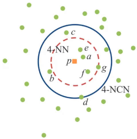
(3) A regression model based on the nearest centroid neighborhood. When k = 1, the target value assigned to the input sample is the target value indicated by its closest neighbor. For k > 1, the k-NN regression model (k-NNR) estimates the target value f (y) of a new input sample y by averaging the target values of its k nearest neighbors [2, 13, 15]:. f (y) =. k 1X ai k i=1. 3. The second neighbor is not the second nearest neighbor (represented as e); instead, the algorithm picks a point located in the opposite direction of the first neighbor with respect to p so that the centroid of that point and all previously selected neighbors is the closest to p.. (1). where ai denotes the target value of the i-th nearest neighbor.. 2.2 k-NCN regression. c. e a. 4-NN p b. f. g 4-NCN. Let p be a query sample whose k nearest centroid neighbors should be found from a set X = {x1 , . . . , xn }. These k neighbors are such that (a) they are as near p as possible, and (b) their centroid is also as close to p as possible. Both conditions can be satisfied through the iterative procedure given in Algorithm 1.. d. Fig. 1 A comparison between NCN and NN. Algorithm 1 Nearest centroid neighbors 1: 2: 3: 4: 5: 6: 7: 8: 9: 10: 11: 12: 13: 14: 15: 16: 17: 18: 19: 20: 21: 22: 23: 24: 25: 26:. Input: X = {x1 , . . . , xn } {Input data set} k {Neighborhood size} p {Query point} Output: Q = {q1 , . . . , qk } {Nearest centroid neighbors} Q←∅ q1 ← findNN(X, p) {q1 is the nearest neighbor} Q ← {q1 } Aux ← X − {q1 } j←1 while j < k do j ←j+1 dist ← ∞ for all xi ∈ Aux do M ← computeCentroid(Q ∪ {xi }) if computeDist(M, p) < dist then q j ← xi end if end for Q ← Q ∪ {qj } Aux ← Aux − {qj } end while. The algorithm is better illustrated through a simple example in Fig. 1. The first neighbor of a query point p, which is denoted by the letter a, corresponds to its first nearest neighbor.. This definition leads to a type of neighborhood in which both closeness and spatial distribution of neighbors are taken into account because of the symmetry (centroid) criterion. Besides, the proximity of the nearest centroid neighbors to the sample is guaranteed because of the incremental nature of the way in which those are obtained from the first nearest neighbor. However, note that the iterative procedure outlined in Algorithm 1 does not minimize the distance to the centroid because it gives precedence to the individual distances instead. On the other hand, the region of influence of the NCN results bigger than that of the traditional nearest neighborhood; as can be seen in Fig. 1, the four nearest centroid neighbors (a, b, c, d) of a point p enclose a region quite bigger than the region defined by the four nearest neighbors (a, e, f, g). For a set of cardinality n, computation of one nearest centroid neighbor of any point requires at most n centroid and distance computations, and also n comparisons to find the minimum of the distances. Therefore k nearest centroid neighbors of a point can be computed in O(kN ) time, which is the same as that required for the computation of k nearest neighbors..

(4) 4. From the concept of nearest centroid neighborhood, it is possible to introduce an alternative regression model, namely k-NCNR, which estimates the output of a query sample y as follows: 1. Find the k nearest centroid neighbors of y by using Algorithm 1. 2. Estimate the target value of y as the average of the target values of its k neighbors by means of Eq. 1.. 3 Experiments The main purpose of the experiments in this study is two-fold. First, we want to establish whether or not the proposed k-NCNR model outperforms the classical k-NNR algorithm. Second, we are also interested in evaluating the performance of the best k-NCNR and k-NNR algorithms in comparison with two support vector regression methods. Experimentation was carried out over a collection of 31 data sets with a wide variety of characteristics in terms of number of attributes and samples. All these data sets were taken from the KEEL repository [1] and their main characteristics are summarized in Table 1. The 5-fold cross-validation procedure was adopted for the experiments because it provides some advantages over other resampling strategies, such as bootstrap with a high computational cost or re-substitution with a biased behavior [18]. The original data set was randomly divided into five stratified segments or folds of (approximately) equal size; for each fold, four blocks were used to fit the model, and the remaining portion was held out for evaluation as an independent test set. Then the results reported here correspond to the averages across the five trials. The main hyper-parameters of the regression models used in the experiments are listed in Table 2. Note that two support vector regression (SVR) algorithms [21], with linear and RBF kernels, were also employed as reference solutions for comparison purposes.. V. Garcı́a et al.. Table 1 Characteristics of the data sets used in the experiments. (1) (2) (3) (4) (5) (6) (7) (8) (9) (10) (11) (12) (13) (14) (15) (16) (17) (18) (19) (20) (21) (22) (23) (24) (25) (26) (27) (28) (29) (30) (31). Diabetes Ele-1 Plastic Quake Laser Ele-2 AutoMPG6 Friedman Delta-Ail MachCPU Dee AutoMPG8 Anacalt Concrete Abalone California Stock Wizmir Wankara MV ForestFire Treasury Mortgage Baseball House Elevators Compact Pole Puma32h Ailerons Tic. #Samples. #Attributes. 43 495 1650 2178 993 1056 392 1200 7129 209 365 392 4052 1030 4177 20640 950 1461 1609 40768 517 1049 1049 337 22784 16599 8192 14998 8192 13750 9822. 2 2 2 3 4 4 5 5 5 6 6 7 7 8 8 8 9 9 9 10 12 15 15 16 16 18 21 26 32 40 85. Table 2 Parameters of the regression algorithms Method. Learning Parameters. k-NCNR. k =1, 3, . . . , 29; Euclidean distance k =1, 3, . . . , 29; Euclidean distance Complexity parameter = 1; linear kernel (polynomial of degree 1); sequential minimal optimization algorithm; epsilon round-off error = 1×1012 ; epsilon insensitive loss function = 0.001; tolerance = 0.001 Complexity parameter = 1; RBF kernel; sequential minimal optimization algorithm; gamma = 0.01; epsilon round-off error = 1×1012 ; epsilon insensitive loss function = 0.001; tolerance = 0.001. k-NNR SVR(L1). SVR(RBF). 3.1 Evaluation criteria In the framework of regression, the purpose of most performance evaluation scores is to estimate how much the predictions (p1 , p2 , . . . , pn ). deviate from the target values (a1 , a2 , . . . , an ). These metrics are minimized when the predicted value for each query sample agrees with its true value [4]. Probably, the most popular measure.

(5) A regression model based on the nearest centroid neighborhood. that has extensively been used to evaluate the performance of a regression model is the root mean square error (RMSE), v u n u1 X RM SE = t (pi − ai )2 n i=1. (2). This metric indicates how far the predicted values pi are from the target values ai by averaging the magnitude of individual errors without taking care of their sign. From the RMSE, we defined the error normalized difference, which is computed for each data set i and each neighborhood size k as follows:. Dif ferrori,k =. RM SEN Ni,k − RM SEN CNi,k RM SEN Ni,k (3). where RM SEN Ni,k and RM SEN CNi,k represent the RMSE achieved on data set i using k-NNR and k-NCNR, respectively. In practice, Dif ferrori,k can be considered as an indicator of improvement or deterioration of the k-NCNR method with respect to the kNNR model: – if Dif ferrori,k > 0, k-NCNR is better than k-NNR; – if Dif ferrori,k < 0, k-NCNR is worse than k-NNR; – if Dif ferrori,k ≈ 0, there are no significant differences between k-NNR and k-NCNR.. 3.2 Non-parametric statistical tests When comparing the results of two or more models over multiple data sets, a non-parametric statistical test is more appropriate than a parametric one because the former is not based on any assumption such as normality or homogeneity of variance [9, 11]. Both pairwise and multiple comparisons were used in this paper. First, we applied the Friedman’s test to discover any statistically significant differences among all the regression models. This starts by ranking the algorithms for each data set independently according to the RMSE results: as there are 30 competing models (15 k-NNR and 15 k-NCNR), the ranks for each data set are from 1 (best) to 30 (worst).. 5. Then the average rank of each algorithm across all data sets is computed. As the Friedman’s test only detects significant differences over the whole pool of comparisons, we then proceeded with the Holm’s post-hoc test in order to compare a control algorithm (the best model) against the remaining techniques by defining a collection of hypothesis around the control method. Afterwards, the Wilcoxon’s paired signedrank test was employed to find out whether or not there exist significant differences between each pair of the five top k-NNR and k-NCNR algorithms. This statistic ranks the differences in performance of two algorithms for each data set, ignoring the signs, and compares the ranks for the positive and the negative differences. In summary, the statistical tests were used as follows: (i) the Friedman’s test was employed over all the models; (ii) the Wilcoxon’s, Friedman’s and Holm’s post-hoc tests were applied to the five top-ranked k-NNR and k-NCNR algorithms with the aim of concentrating the analysis on the best results of each approach.. 4 Results This section is divided into two blocks. First, the comparison between the k-NCNR and kNNR models is discussed in Section 4.1. Second, the results of the best configurations of k-NCNR and k-NNR are compared against the results of the SVR models in Section 4.2. The detailed results obtained over each data set and each algorithm are reported in Tables 8 and 9 in the Appendix.. 4.1 k-NCNR vs k-NNR Figure 2 depicts the error normalized difference for each database (i = 1, . . . , 31) with all neighborhood sizes. The most important observation is that a vast majority of cases achieved positive values (Dif ferrori,k > 0), indicating that the performance of the k-NCNR model was superior to that of the corresponding k-NNR algorithm for most databases. Figure 3 shows the Friedman’s average ranks achieved from the RMSE results with all the regression methods (k-NNR and k-NCNR). As can be observed, the lowest (best) average ranks.

(6) 6. V. Garcı́a et al.. Fig. 2 Error normalized difference on the 31 data sets. were achieved with both strategies using k values in the range from 9 to 21. More specifically, the best k-NNR configurations were with k = 9, 11, 17, 13, 15, whose ranks were 6.4194, 6.7097, 6.7903, 6.9032 and 6.9032 respectively. In the case of k-NCNR, the best k values were 11, 19, 21, 9 and 13 with ranks 7.0323, 7.1935, 7.2581, 7.3226 and 7.3871 respectively.. less chance), and the lower diagonal half corresponds to a significance level of α = 0.05. The symbol “•” indicates that the method in the row significantly outperforms the method in the column, whereas the symbol “◦” means that the method in the column performs significantly better than the method in the row. Table 3 Summary of the Wilcoxon’s statistic for the best k-NNR and k-NCNR models. Upper and lower diagonal halves are for α = 0.10 and α = 0.05, respectively (1) (2) (3) (4) (5) (6) (7) (8) (9) (10) (1) (2) (3) (4) (5) (6) (7) (8) (9) (10). Fig. 3 Friedman’s ranks of the k-NNR and k-NCNR models. Table 3 reports the results of the Wilcoxon’s test applied to the ten best regression models. The upper diagonal half summarizes this statistic at a significance level of α = 0.10 (10% or. 9-NNR 11-NNR 17-NNR 13-NNR 15-NNR 11-NCNR 19-NCNR 21-NCNR 9-NCNR 13-NCNR. – – – – • • •. • • • • •. • • • • •. • • • • •. – • • • • •. ◦ ◦ ◦ ◦ ◦ –. ◦ ◦ ◦ ◦. ◦ ◦ ◦ ◦. ◦ ◦ ◦ ◦ ◦. ◦ ◦ ◦ ◦ ◦. – – – –. Analysis of the results in Table 3 allows to remark that the k-NCNR models were significantly better than the k-NNR algorithms. On the other hand, it is also interesting to note that different values of k did not yield statistically significant differences between pairs of the same strategy; for instance, in the case of k-NCNR, there was no neighborhood size performing significantly better than some other value of k..

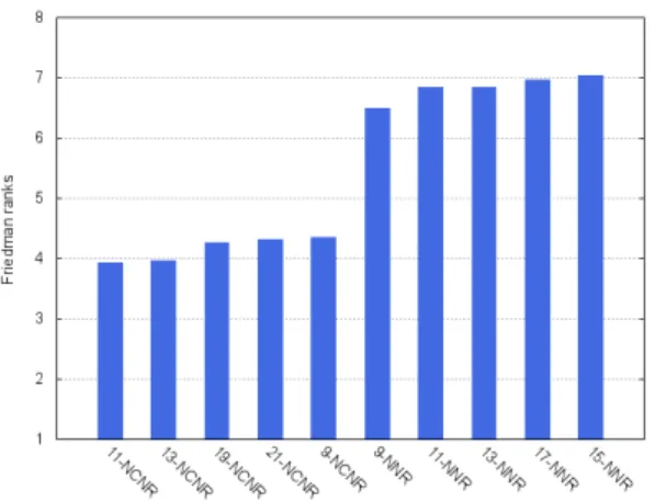
(7) A regression model based on the nearest centroid neighborhood. Because the Wilcoxon’s test for multiple comparisons do not allow to conclude which algorithm is the best, we applied a Friedman’s test to the five top-ranked k-NNR and k-NCNR approaches and afterwards, a Holm’s post-hoc test in order to determine whether or not there exists significant differences with the best (control) model. As we had 10 algorithms and 31 databases, the Friedman’s test using the ImanDavenport statistic, which is distributed according to the F -distribution with 10 − 1 = 9 and (10 − 3)(31 − 1) = 270 degrees of freedom, was 8.425717. The p-value calculated by F (9, 270) was 4.3×10−11 and therefore, the null-hypothesis that all algorithms performed equally well can be rejected with a high significance level. Figure 4 depicts the Friedman’s average rankings for the five top-ranked k-NNR and k-NCNR algorithms. One can see that the approach with the best scores corresponds to 11-NCNR, which will be the control algorithm for the subsequent Holm’s post-hoc test. It is also worth pointing out that all the k-NCNR models achieved lower rankings than the k-NNR methods, proving the superiority of the surrounding neighborhood to the conventional neighborhood,. 7. ject the null-hypothesis of equivalence between 11-NCNR and the rest of k-NCNR algorithms. Table 4 Unadjusted p-values for α = 0.05 and α = 0.10 with 11-NCNR as the control algorithm. The models in bold were significantly worse than the control algorithm z 15-NNR 17-NNR 21-NNR 13-NNR 9-NNR 9-NCNR 21-NCNR 19-NCNR 13-NCNR. 4.026889 3.942996 3.775209 3.775209 3.313794 0.545308 0.503361 0.419468 0.041947. p-value α = 0.05/i α = 0.10/i 0.000057 0.000080 0.000160 0.000160 0.000920 0.585542 0.614710 0.674874 0.966541. 0.005556 0.006250 0.007143 0.008333 0.010000 0.012500 0.016667 0.025000 0.050000. 0.011111 0.012500 0.014286 0.016667 0.020000 0.025000 0.033333 0.050000 0.100000. 4.2 Neighborhood-based regression models vs SVR This section analyzes the results of the two top k-NCNR and k-NNR algorithms with respect to two SVR algorithms. The average RMSE results of these models on the 31 data sets and the Friedman’s average rankings are reported in Table 5. Friedman’s average ranks for the four regressions models have been plotted in Fig.5. As can be seen, both 11-NCNR and SVR(L1) arose as the algorithms with the lowest rankings, that is, the lowest RMSE in average.. Fig. 4 Friedman’s ranks of the five best results for the k-NNR and k-NCNR models.. Table 4 reports the results of the Holm’s test using 11-NCNR as the control algorithm, including the z value, the unadjusted p-value, and the adjusted α value at significance levels of 0.05 and 0.10. It can be viewed that 11NCNR was significantly better than the five top-ranked k-NNR models at both significance levels. On the contrary, it is not possible to re-. Fig. 5 Friedman’s ranks of two best k-NCNR and k-NNR benchmarked methods and two SVR models.. In order to check whether or not the RMSE results were significantly different, the ImanDavenport’s statistic was computed. This is distributed according to an F -distribution with 3.

(8) 8. V. Garcı́a et al.. Table 5 Average RMSE results of two SVR models and the best neighborhood-based algorithms. Diabetes Ele-1 Plastic Quake Laser Ele-2 AutoMPG6 Friedman Delta-Ail MachCPU Dee AutoMPG8 Anacalt Concrete Abalone California Stock Wizmir Wankara MV ForestFire Treasury Mortgage Baseball House Elevators Compact Pole Puma32H Ailerons Tic Avg. Ran.. SVR(L1). SVR(RBF) 11-NCNR 9-NNR. 5.88×10−1 6.40×102 1.53×100 2.04×10−1 2.34×101 1.68×102 3.55×100 2.71×100 1.74×10−4 6.98×101 4.08×10−1 3.45×100 5.15×10−1 1.11×101 2.27×100 7.08×104 2.39×100 1.26×100 1.57×100 5.31×100 5.71×101 2.48×10−1 5.31×100 7.57×102 4.77×104 2.97×10−3 1.24×101 3.10×101 2.71×10−2 1.77×10−4 2.44×10−1. 6.62×10−1 7.64×102 2.19×100 2.04×10−1 2.46×101 2.16×102 3.67×100 2.69×100 1.76×10−4 9.03×101 4.23×10−1 3.61×100 5.14×10−1 1.09×101 2.40×100 7.33×104 2.48×100 1.27×100 1.58×100 2.35×100 5.71×101 2.85×10−1 2.35×100 7.76×102 4.79×104 2.93×10−3 1.35×101 3.28×101 2.70×10−2 1.70×10−4 2.44×10−1. 6.16×10−1 6.41×102 1.59×100 1.94×10−1 1.06×101 1.19×102 3.88×100 1.68×100 1.85×10−4 8.04×101 4.02×10−1 3.92×100 7.67×10−2 7.91×100 2.12×100 9.17×104 9.23×10−1 1.31×100 1.36×100 6.08×100 5.87×101 5.44×10−1 3.72×10−1 9.08×102 5.02×104 6.35×10−3 6.23×100 8.20×100 2.79×10−2 3.00×10−4 2.39×10−1. 6.31×10−1 6.41×102 1.63×100 1.95×10−1 1.14×101 1.60×102 4.14×100 1.81×100 1.90×10−4 7.53×101 4.22×10−1 4.20×100 7.80×10−2 9.64×100 2.20×100 9.67×104 8.46×10−1 1.45×100 1.48×100 7.07×100 5.97×101 5.17×10−1 3.54×10−1 8.92×102 5.07×104 6.56×10−3 6.50×100 8.33×100 2.82×10−2 3.49×10−4 2.41×10−1. 2.16. 2.87. 2.16. 2.81. We run a Wilcoxon’s paired signed-rank test for α = 0.05 and α = 0.10 between each pair of regression algorithms. From Table 7, we can observe that 11-NCNR performed significantly better than 9-NNR at both significance levels, and it was significantly better than SVR(RBF) at α = 0.10. On the other hand, it also has to be noted that SVR(L1) was significantly better than the SVR model with an RBF kernel at α = 0.10 and α = 0.05. This suggests that, for regression problems, we can use either kNCNR or the linear SVR, since both these models yielded equivalent performance results.. Table 7 Summary of the Wilcoxon’s statistic for the best k-NNR and k-NCNR models, and two SVR algorithms. Upper and lower diagonal halves are for α = 0.10 and α = 0.05, respectively (1) (2) (3) (4) (1) (2) (3) (4). 11-NCNR 9-NNR SVR(L1) SVR(RBF). . . -. . -. 5 Conclusions and future work and 90 degrees of freedom. The p-value computed was 0.03275984862, which is less than a significance level of α=0.05. Therefore, the nullhypothesis that all regression models performed equally well can be rejected. Table 6 shows the unadjusted p-values for a Holm’s post hoc test using the 11-NCNR algorithm as the control method. For a significance level of α=0.05, the procedure could not reject the null-hypothesis of equivalence in any of the three algorithms. Conversely, at a significance level of α=0.10, the Holm’s test indicates that 11-NCNR was significantly better than 9-NNR and SVR(RBF), and equivalent to SVR(L1).. Table 6 Unadjusted p-values for α = 0.05 and α = 0.10 with 11-NCNR as the control algorithm when compared against 9-NNR, SVR(L1), and SVR(RBF). The model in bold was significantly worse than the control algorithm at α = 0.10. z. p-value α = 0.05/i α = 0.10/i. SVR(RBF) 2.164225 0.030447 9-NNR 1.967478 0.049128 SVR(L1) 0 1. 0.016667 0.025 0.05. 0.033333 0.05 0.10. In this paper, a new regression technique based on the nearest centroid neighborhood has been introduced. The general idea behind this strategy is that neighbors of a query sample should fulfill two complementary conditions: proximity and symmetry. In order to discover the applicability of this regression model, it has been compared to the k-NNR algorithm when varying the neighborhood size k from 1 to 29 (using only the odd values) and two configurations of SVR (with linear and RBF kernels) over a total of 31 databases. The experimental results in terms of RMSE (and the error normalized difference proposed here) have shown that the k-NCNR model is statistically better than the k-NNR method. In particular, the best results have been achieved with values of k in the range from 9 to 21 and more specifically, the 11-NCNR approach has outperformed the five top-ranked k-NNR algorithms. When compared against the two SVR models, the results have suggested that the kNCNR algorithm performs equally well as the linear SVR and better than SVR(RBF)..

(9) A regression model based on the nearest centroid neighborhood. It is also important to note that the k-NCNR model is a lazy algorithm that does not require any training, which can constitute an interesting advantage over the SVR methods for big data applications. Several promising directions for further research have emerged from this study. First, a natural extension is to develop regression models based on other surrounding neighborhoods such as those defined from the Gabriel graph and the relative neighborhood graph, which are two well-known proximity graphs. Second, it would be interesting to assess the performance of the k-NCNR algorithm and compared to other regression models when applied to some real-life problem. Acknowledgements This work has partially been supported by the Generalitat Valenciana under grant [PROMETEOII/2014/062] and the Spanish Ministry of Economy, Industry and Competitiveness under grant [TIN2013-46522-P].. References 1. Alcalá-Fdez, J., Fernández, A., Luengo, J., Derrac, J., Garcı́a, S., Sánchez, L., Herrera, F.: KEEL data-mining software tool: Data set repository, integration of algorithms and experimental analysis framework. J Mult-Valued Log S 17, 255–287 (2011) 2. Biau, G., Devroye, L., Dujimovič, V., Krzyzak, A.: An affine invariant -nearest neighbor regression estimate. J Multivariate Anal 112, 24–34 (2012) 3. Buza, K., Nanopoulos, A., Nagy, G.: Nearest neighbor regression in the presence of bad hubs. Knowl-Based Syst 86, 250–260 (2015) 4. Caruana, R., Niculescu-Mizil, A.: Data mining in metric space: An empirical analysis of supervised learning performance criteria. In: 10th ACM SIGKDD International Conference on Knowledge Discovery and Data Mining, pp. 69–78. New York, NY (2004) 5. Chaudhuri, B.: A new definition of neighborhood of a point in multi-dimensional space. Pattern Recogn Lett 17(1), 11–17 (1996) 6. Cheng, C.B., Lee, E.: Nonparametric fuzzy regression—k-nn and kernel smoothing techniques. Comput Math Appl 38(3–4), 239–251 (1999) 7. Dasarathy, B.: Nearest Neighbor (NN) Norms: NN Pattern Classification Techniques. IEEE Computer Society Press, Los Alomitos, CA (1990) 8. Dell’Acqua, P., Belloti, F., Berta, R., Gloria, A.D.: Time-aware multivariate nearest neighbor regression methods for traffic flow prediction. IEEE T Intell Transp 16(6), 3393–3402 (2015) 9. Demšar, J.: Statistical comparisons of classifiers over multiple data sets. J Mach Learn Res 7, 1–30 (2006). 9. 10. Eronen, A.J., Klapuri, A.P.: Music tempo estimation with k-nn regression. IEEE T Audio Speech 18(1), 50–57 (2010) 11. Garcı́a, S., Fernández, A., Luengo, J., Herrera, F.: Advanced nonparametric tests for multiple comparisons in the design of experiments in computational intelligence and data mining: Experimental analysis of power. Inform Sciences 130, 2044–2064 (2010) 12. Garcı́a, V., Sánchez, J. S., Martı́n-Félez, R., Mollineda, R. A.: Surrounding neighborhoodbased SMOTE for learning from imbalanced data sets. Progr Artif Int 1(4), 347–362 (2012) 13. Guyader, A., Hengartner, N.: On the mutual nearest neighbors estimate in regression. J Mach Learn Res 14, 2361–2376 (2013) 14. Hu, C., Jain, G., Zhang, P., Schmidt, C., Gomadam, P., Gorka, T.: Data-driven method based on particle swarm optimization and knearest neighbor regression for estimating capacity of lithium-ion battery. Appl Energ 129, 49– 55 (2014) 15. Lee, S.Y., Kang, P., Cho, S.: Probabilistic local reconstruction for k-nn regression and its application to virtual metrology in semiconductor manufacturing. Neurocomputing 131, 427–439 (2014) 16. Leon, F., Popescu, E.: Using large margin nearest neighbor regression algorithm to predict student grades based on social media traces. In: International Conference in Methodologies and Intelligent Systems for Technology Enhanced Learning, pp. 12–19. Porto, Portugal (2017) 17. Mack, Y.P.: Local properties of k-nn regression estimates. SIAM J Algebra Discr 2(3), 311–323 (1981) 18. Ounpraseuth, S., Lensing, S.Y., Spencer, H.J., Kodell, R.L.: Estimating misclassification error: a closer look at cross-validation based methods. BMC Res Notes 5(656), 1–12 (2012) 19. Sánchez, J.S., Marqués, A.I.: Enhanced neighbourhood specifications for pattern classification. In: Pattern Recognition and String Matching, pp. 673–702 (2002) 20. Sánchez, J.S., Pla, F., Ferri, F.J.:Improving the k-NCN classification rule through heuristic modifications. Pattern Recogn Lett 19(13), 1165– 1170 (1998) 21. Shevade, S.K., Keerthi, S.S., Bhattacharyya, C., Murthy, K.R.K.: Improvements to the SMO algorithm for SVM regression. IEEE T Neural Networ 11(5), 1188–1193 (2000) 22. Song, Y., Liang, J., Lu, J., Zhao, X.: An efficient instance selection algorithm for k nearest neighbor regression. Neurocomputing 251(16), 26–34 (2017) 23. Treiber, N., Kramer, O.: Evolutionary feature weighting for wind power prediction with nearest neighbor regression. In: IEEE Congress on Evolutionary Computation, pp. 332–337. Sendai, Japan (2015) 24. Xiao, Y., Griffin, M.P., Lake, D.E., Moorman, J.R.: Nearest-neighbor and logistic regression analyses of clinical and heart rate characteristics in the early diagnosis of neonatal sepsis. Med Decis Making 30(2), 258–266 (2010).

(10) 10. 25. Yang, S., Zhao, C.: Regression nearest neighbor in face recognition. In: 18th International Conference on Pattern Recognition, pp. 515–518. Hong Kong, China (2006) 26. Yao, Z., Ruzo, W.: A regression-based k nearest neighbor algorithm for gene function prediction from heterogeneous data. BMC Bioinformatics 7(1), 1–11 (2006) 27. Yu, J., Hong, C.: Exemplar-based 3D human pose estimation with sparse spectral embedding. Neurocomputing 269, 82–89 (2017) 28. Zhang, J., Yim, Y.S., Yang, J.: Intelligent selection of instances for prediction functions in lazy learning algorithms. Artif Intell Rev 11(1–5), 175–191 (1997). Appendix Tables 8 and 9 report the average RMSE results for all the data sets and for each value of k. In addition, the Friedman’s rankings are given in the last row of each table.. V. Garcı́a et al..

(11) 10.03. Avg. Ran.. 11.77. 6.84×10−1 6.41×102 1.86×100 2.10×10−1 9.40×100 1.19×102 4.33×100 1.94×100 2.03×10−4 5.84×101 4.48×10−1 4.26×100 8.20×10−2 8.90×100 2.34×100 1.04×105 6.84×10−1 1.53×100 1.59×100 7.63×100 6.62×101 3.07×10−1 2.63×10−1 9.64×102 5.46×104 7.09×10−3 7.00×100 7.73×100 3.09×10−2 3.62×10−4 2.61×10−1. 3. Diabetes 8.13×10−1 Ele-1 7.76×102 Plastic 2.21×100 Quake 2.56×10−1 Laser 1.07×101 Ele-2 7.62×101 AutoMPG-6 5.02×100 Friedman 2.49×100 Delta-Ail 2.52×10−4 MachineCPU 6.10×101 Dee 5.46×10−1 AutoMPG-8 4.94×100 Anacalt 1.02×10−1 Concrete 8.97×100 Abalone 2.84×100 California 1.26×105 Stock 7.24×10−1 Wizmir 1.86×100 Wankara 1.94×100 MV 9.22×100 ForestFires 1.04×102 Treasury 3.29×10−1 Mortgage 2.83×10−1 Baseball 1.22×103 House 6.42×104 Elevators 8.67×10−3 Compactiv 8.50×100 Pole 8.36×100 Puma32H 3.79×10−2 Ailerons 4.36×10−4 Tic 3.18×10−1. 1. 8.84. 6.50×10−1 6.42×102 1.72×100 2.01×10−1 9.92×100 1.47×102 4.22×100 1.84×100 1.95×10−4 6.43×101 4.34×10−1 4.23×100 7.87×10−2 9.16×100 2.24×100 9.96×104 7.44×10−1 1.50×100 1.50×100 7.29×100 6.22×101 3.55×10−1 2.85×10−1 9.24×102 5.26×104 6.77×10−3 6.71×100 7.84×100 2.93×10−2 3.52×10−4 2.49×10−1. 5. 7.07. 6.40×10−1 6.41×102 1.67×100 1.97×10−1 1.07×101 1.47×102 4.13×100 1.80×100 1.91×10−4 7.07×101 4.24×10−1 4.21×100 7.83×10−2 9.41×100 2.21×100 9.76×104 8.03×10−1 1.46×100 1.49×100 7.14×100 6.10×101 4.48×10−1 3.11×10−1 9.06×102 5.14×104 6.62×10−3 6.56×100 8.12×100 2.86×10−2 3.49×10−4 2.43×10−1. 7. 6.42. 6.31×10−1 6.41×102 1.63×100 1.95×10−1 1.14×101 1.60×102 4.14×100 1.81×100 1.90×10−4 7.53×101 4.22×10−1 4.20×100 7.80×10−2 9.64×100 2.20×100 9.67×104 8.46×10−1 1.45×100 1.48×100 7.07×100 5.97×101 5.17×10−1 3.54×10−1 8.92×102 5.07×104 6.56×10−3 6.50×100 8.33×100 2.82×10−2 3.49×10−4 2.41×10−1. 9. 6.71. 6.54×10−1 6.55×102 1.59×100 1.93×10−1 1.22×101 1.68×102 4.11×100 1.84×100 1.88×10−4 8.11×101 4.22×10−1 4.20×100 7.68×10−2 9.89×100 2.19×100 9.62×104 8.96×10−1 1.45×100 1.49×100 7.04×100 5.82×101 5.95×10−1 4.20×10−1 9.02×102 5.04×104 6.53×10−3 6.43×100 8.67×100 2.79×10−2 3.49×10−4 2.39×10−1. 11. 6.90. 6.59×10−1 6.54×102 1.57×100 1.92×10−1 1.26×101 1.77×102 4.14×100 1.83×100 1.87×10−4 8.60×101 4.22×10−1 4.23×100 7.70×10−2 1.00×101 2.19×100 9.59×104 9.12×10−1 1.45×100 1.50×100 7.02×100 5.73×101 6.55×10−1 4.73×10−1 9.18×102 5.01×104 6.51×10−3 6.39×100 9.00×100 2.78×10−2 3.50×10−4 2.38×10−1. 13. 6.90. 6.43×10−1 6.54×102 1.56×100 1.91×10−1 1.29×101 1.79×102 4.17×100 1.86×100 1.88×10−4 8.99×101 4.25×10−1 4.27×100 7.67×10−2 1.02×101 2.19×100 9.56×104 9.41×10−1 1.45×100 1.51×100 7.00×100 5.69×101 7.08×10−1 5.30×10−1 9.17×102 4.99×104 6.50×10−3 6.38×100 9.28×100 2.76×10−2 3.52×10−4 2.38×10−1. 15. 6.79. 6.34×10−1 6.62×102 1.55×100 1.91×10−1 1.32×101 1.86×102 4.17×100 1.90×100 1.87×10−4 9.26×101 4.24×10−1 4.24×100 7.65×10−2 1.03×101 2.18×100 9.56×104 9.73×10−1 1.45×100 1.54×100 7.01×100 5.68×101 7.63×10−1 5.75×10−1 9.20×102 4.97×104 6.49×10−3 6.39×100 9.49×100 2.75×10−2 3.53×10−4 2.37×10−1. 17. 7.07. 6.39×10−1 6.70×102 1.55×100 1.91×10−1 1.36×101 1.96×102 4.19×100 1.95×100 1.87×10−4 9.46×101 4.28×10−1 4.22×100 7.65×10−2 1.05×101 2.19×100 9.55×104 1.01×100 1.44×100 1.54×100 7.01×100 5.64×101 8.07×10−1 6.21×10−1 9.26×102 4.96×104 6.48×10−3 6.38×100 9.72×100 2.74×10−2 3.55×10−4 2.36×10−1. 19. 7.03. 6.41×10−1 6.66×102 1.54×100 1.91×10−1 1.38×101 2.08×102 4.17×100 1.97×100 1.87×10−4 9.69×101 4.29×10−1 4.20×100 7.69×10−2 1.07×101 2.19×100 9.54×104 1.04×100 1.45×100 1.55×100 7.01×100 5.66×101 8.40×10−1 6.61×10−1 9.26×102 4.95×104 6.48×10−3 6.37×100 9.93×100 2.74×10−2 3.56×10−4 2.36×10−1. 21. 8.06. 6.49×10−1 6.68×102 1.54×100 1.90×10−1 1.41×101 2.17×102 4.19×100 2.00×100 1.87×10−4 9.94×101 4.32×10−1 4.21×100 7.75×10−2 1.09×101 2.20×100 9.54×104 1.06×100 1.46×100 1.57×100 7.02×100 5.68×101 8.69×10−1 6.84×10−1 9.28×102 4.94×104 6.47×10−3 6.38×100 1.01×101 2.73×10−2 3.57×10−4 2.36×10−1. 23. 8.13. 6.57×10−1 6.68×102 1.54×100 1.90×10−1 1.42×101 2.30×102 4.19×100 2.02×100 1.87×10−4 1.01×102 4.31×10−1 4.18×100 7.79×10−2 1.10×101 2.20×100 9.54×104 1.09×100 1.47×100 1.58×100 7.02×100 5.65×101 8.93×10−1 7.06×10−1 9.36×102 4.93×104 6.47×10−3 6.37×100 1.03×101 2.73×10−2 3.58×10−4 2.35×10−1. 25. 8.79. 6.65×10−1 6.62×102 1.54×100 1.90×10−1 1.44×101 2.41×102 4.18×100 2.04×100 1.87×10−4 1.03×102 4.31×10−1 4.17×100 7.83×10−2 1.10×101 2.20×100 9.55×104 1.11×100 1.48×100 1.60×100 7.03×100 5.62×101 9.17×10−1 7.25×10−1 9.39×102 4.93×104 6.47×10−3 6.37×100 1.05×101 2.73×10−2 3.59×10−4 2.35×10−1. 27. 9.48. 6.81×10−1 6.67×102 1.54×100 1.90×10−1 1.46×101 2.50×102 4.17×100 2.06×100 1.87×10−4 1.05×102 4.34×10−1 4.16×100 7.91×10−2 1.11×101 2.21×100 9.55×104 1.14×100 1.49×100 1.61×100 7.03×100 5.62×101 9.41×10−1 7.42×10−1 9.40×102 4.92×104 6.47×10−3 6.38×100 1.07×101 2.72×10−2 3.61×10−4 2.35×10−1. 29. Table 8 Average RMSE results on 31 real regression data sets with k-NNR . The average Friedman ranks for each k value are shown in the last row.. A regression model based on the nearest centroid neighborhood 11.

(12) 10.16. 12.29. Avg. Ran.. 3. 6.32×10−1 6.74×102 1.85×100 2.09×10−1 7.94×100 1.09×102 4.24×100 1.69×100 2.04×10−4 5.79×101 4.24×10−1 4.15×100 8.38×10−2 7.29×100 2.37×100 1.02×105 6.36×10−1 1.42×100 1.47×100 7.21×100 6.66×101 2.91×10−1 2.24×10−1 9.80×102 5.47×104 7.05×10−3 6.90×100 7.01×100 3.07×10−2 3.40×10−4 2.61×10−1. Diabetes 8.13×10−1 Ele-1 7.76×102 Plastic 2.21×100 Quake 2.56×10−1 Laser 1.07×101 Ele-2 7.62×101 AutoMPG-6 5.02×100 Friedman 2.49×100 Delta-Ail 2.52×10−4 MachineCPU 6.10×101 Dee 5.46×10−1 AutoMPG-8 4.94×100 Anacalt 1.02×10−1 Concrete 8.97×100 Abalone 2.84×100 California 1.26×105 Stock 7.24×10−1 Wizmir 1.86×100 Wankara 1.94×100 MV 9.22×100 ForestFires 1.04×102 Treasury 3.29×10−1 Mortgage 2.83×10−1 Baseball 1.22×103 House 6.42×104 Elevators 8.67×10−3 Compactiv 8.50×100 Pole 8.36×100 Puma32H 3.79×10−2 Ailerons 4.36×10−4 Tic 3.18×10−1. 1. 8.68. 6.13×10−1 6.44×102 1.72×100 2.00×10−1 8.86×100 1.09×102 4.08×100 1.60×100 1.95×10−4 6.53×101 4.01×10−1 4.08×100 7.94×10−2 7.36×100 2.22×100 9.64×104 7.34×10−1 1.34×100 1.35×100 6.67×100 6.38×101 3.58×10−1 2.48×10−1 9.50×102 5.24×104 6.67×10−3 6.57×100 7.20×100 2.92×10−2 3.19×10−4 2.49×10−1. 5. 7.61. 6.00×10−1 6.50×102 1.66×100 1.97×10−1 9.62×100 1.06×102 3.93×100 1.64×100 1.90×10−4 7.44×101 3.98×10−1 4.00×100 7.72×10−2 7.47×100 2.18×100 9.40×104 7.83×10−1 1.28×100 1.33×100 6.40×100 6.31×101 4.34×10−1 2.88×10−1 9.21×102 5.12×104 6.50×10−3 6.39×100 7.57×100 2.85×10−2 3.08×10−4 2.43×10−1. 7. 7.32. 6.04×10−1 6.45×102 1.63×100 1.96×10−1 1.02×101 1.11×102 3.86×100 1.66×100 1.87×10−4 7.85×101 3.97×10−1 3.97×100 7.69×10−2 7.63×100 2.14×100 9.26×104 8.56×10−1 1.29×100 1.32×100 6.22×100 6.00×101 5.01×10−1 3.36×10−1 9.22×102 5.06×104 6.41×10−3 6.31×100 7.86×100 2.81×10−2 3.03×10−4 2.41×10−1. 9. 7.03. 6.16×10−1 6.41×102 1.59×100 1.94×10−1 1.06×101 1.19×102 3.88×100 1.68×100 1.85×10−4 8.04×101 4.02×10−1 3.92×100 7.67×10−2 7.91×100 2.12×100 9.17×104 9.23×10−1 1.31×100 1.36×100 6.08×100 5.87×101 5.44×10−1 3.72×10−1 9.08×102 5.02×104 6.35×10−3 6.23×100 8.20×100 2.79×10−2 3.00×10−4 2.39×10−1. 11. 7.39. 6.41×10−1 6.35×102 1.56×100 1.93×10−1 1.12×101 1.27×102 3.88×100 1.72×100 1.85×10−4 8.51×101 4.02×10−1 3.92×100 7.77×10−2 8.04×100 2.10×100 9.11×104 9.83×10−1 1.30×100 1.35×100 5.99×100 5.89×101 5.80×10−1 4.13×10−1 9.12×102 4.99×104 6.31×10−3 6.20×100 8.47×100 2.77×10−2 2.98×10−4 2.37×10−1. 13. 7.45. 6.43×10−1 6.36×102 1.54×100 1.93×10−1 1.15×101 1.35×102 3.87×100 1.76×100 1.84×10−4 8.79×101 4.02×10−1 3.94×100 7.72×10−2 8.14×100 2.10×100 9.07×104 1.02×100 1.30×100 1.36×100 5.93×100 5.93×101 6.22×10−1 4.46×10−1 9.12×102 4.97×104 6.27×10−3 6.17×100 8.77×100 2.76×10−2 2.96×10−4 2.36×10−1. 15. 7.45. 6.38×10−1 6.31×102 1.53×100 1.92×10−1 1.21×101 1.38×102 3.95×100 1.79×100 1.83×10−4 9.05×101 4.04×10−1 3.96×100 7.79×10−2 8.32×100 2.10×100 9.04×104 1.06×100 1.32×100 1.36×100 5.87×100 5.85×101 6.65×10−1 4.87×10−1 9.01×102 4.95×104 6.26×10−3 6.15×100 9.02×100 2.76×10−2 2.95×10−4 2.35×10−1. 17. 7.19. 6.47×10−1 6.25×102 1.52×100 1.91×10−1 1.24×101 1.51×102 3.96×100 1.84×100 1.83×10−4 9.30×101 4.03×10−1 3.95×100 7.83×10−2 8.42×100 2.09×100 9.01×104 1.09×100 1.33×100 1.37×100 5.83×100 5.77×101 6.99×10−1 5.22×10−1 9.01×102 4.94×104 6.24×10−3 6.14×100 9.26×100 2.75×10−2 2.93×10−4 2.34×10−1. 19. 7.26. 6.48×10−1 6.23×102 1.53×100 1.91×10−1 1.27×101 1.58×102 3.96×100 1.87×100 1.83×10−4 9.27×101 4.08×10−1 3.94×100 7.90×10−2 8.55×100 2.09×100 8.99×104 1.12×100 1.33×100 1.39×100 5.80×100 5.75×101 7.30×10−1 5.61×10−1 9.01×102 4.92×104 6.22×10−3 6.14×100 9.49×100 2.74×10−2 2.93×10−4 2.34×10−1. 21. 7.42. 6.59×10−1 6.27×102 1.53×100 1.90×10−1 1.30×101 1.66×102 3.96×100 1.90×100 1.83×10−4 9.42×101 4.10×10−1 3.94×100 7.96×10−2 8.68×100 2.09×100 8.97×104 1.16×100 1.33×100 1.39×100 5.76×100 5.74×101 7.68×10−1 5.96×10−1 8.95×102 4.92×104 6.21×10−3 6.14×100 9.67×100 2.74×10−2 2.92×10−4 2.34×10−1. 23. 7.42. 6.59×10−1 6.28×102 1.52×100 1.90×10−1 1.33×101 1.75×102 3.96×100 1.94×100 1.82×10−4 9.57×101 4.13×10−1 3.92×100 8.01×10−2 8.80×100 2.10×100 8.96×104 1.19×100 1.33×100 1.40×100 5.73×100 5.72×101 7.98×10−1 6.27×10−1 8.97×102 4.91×104 6.20×10−3 6.13×100 9.86×100 2.74×10−2 2.92×10−4 2.33×10−1. 25. 7.39. 6.65×10−1 6.27×102 1.52×100 1.90×10−1 1.36×101 1.84×102 3.95×100 1.96×100 1.82×10−4 9.78×101 4.14×10−1 3.92×100 8.06×10−2 8.91×100 2.10×100 8.94×104 1.21×100 1.35×100 1.42×100 5.71×100 5.71×101 8.32×10−1 6.56×10−1 9.01×102 4.91×104 6.20×10−3 6.13×100 1.00×101 2.73×10−2 2.91×10−4 2.33×10−1. 27. 7.94. 6.74×10−1 6.31×102 1.51×100 1.90×10−1 1.38×101 1.92×102 3.95×100 1.99×100 1.82×10−4 1.00×102 4.16×10−1 3.93×100 8.10×10−2 9.04×100 2.10×100 8.94×104 1.23×100 1.35×100 1.43×100 5.70×100 5.69×101 8.70×10−1 6.81×10−1 9.04×102 4.91×104 6.20×10−3 6.13×100 1.02×101 2.73×10−2 2.90×10−4 2.33×10−1. 29. Table 9 Average RMSE results on 31 real regression data sets with k-NCNR. The average Friedman ranks for each k value are shown in the last row.. 12 V. Garcı́a et al..

(13)