TítuloFractional order modelling of contact with the environment in flexible robot applications

Texto completo

(1)Actas de las XXXIX Jornadas de Automática, Badajoz, 5-7 de Septiembre de 2018 https://doi.org/10.17979/spudc.9788497497565.0710. FRACTIONAL ORDER MODELLING OF CONTACT WITH THE ENVIRONMENT IN FLEXIBLE ROBOT APPLICATIONS José Emilio Traver1 , Inés Tejado1 , Javier Prieto-Arranz2 , Blas M. Vinagre1 Industrial Engineering School, University of Extremadura, 06006 Badajoz, Spain. email: {jetraverb;itejbal;bvinagre}@unex.es 2 School of Industrial Engineering, University of Castilla-La Mancha, 13071 Ciudad Real, Spain. email: Javier.PrietoArranz@uclm.es 1. Abstract. and links. The first kind appears as a consequent of torsion in the elements that join actuators (motors) and link. For the second kind, the flexibility of links is owing to heavy loads or fast motions. In this case, each link suffers a deformation and, therefore, a change of the position of the tip regarding to the calculated it. In the robotic designs, the second kind is chosen mostly and the flexibility of links allow to reduce its weight and provide a set of significant advantages over the standard rigid robots. A lightweight flexible robot can perform faster movements, is more easily transportable, its payload-to-arm weight ratio is higher and has a lower energy requirements [6].. The control of flexible robots that interact with the environment presents some difficulties because the mechanical environment is unknown. In this kind of applications, force robust control rather than position control is required. The purpose of this paper is to model the mechanical impedance of the environment contacted by a flexible link based on the well-known spring-damper system typically used in the literature, considering models of both integer and fractional order. In particular, four models are identified: 1) linear regression model, 2) spring-damper model, 3) spring-damper model that also includes a spring for the robotic arm, and 4) fractional order extension of spring-damper model. Experimental results (impacts with ten different objects) are given to identify the parameters of the considered models. The goodness of the adjustment is analyzed by a set of performance indices. The results show that fractional models may have better performance in comparison with classical alternatives proposed in the literature for the objects used in this study.. The interaction of flexible manipulators with the environment plays an important role when they carry out tasks. These tasks, which can be classified in free (with no contact with the environment) or constrained (with interaction with the environment), currently require manipulators with some special properties, as mentioned above. This is the reason why flexible manipulators are desirable against rigid robots. The effects of the impact with objects or humans in rigid robots cause that the contact force grows very quickly, reaching very high value. Thus, the collision may produce the deformation or breaking of rigid arm and collided object. However, these effects are reduced in flexible arms owing to a significant part of the kinetic energy of the robots at the collision instant is gradually transformed into elastic potential energy of the robot links. Then, the contact force grows slowly [9, 6]. However, the control problem of flexible manipulators turns more complex [17, 20, 3, 16, 15, 4, 5].. Keywords: Flexible link, Contact, Soft material, Mechanical impedance, Fractional order model.. 1. INTRODUCTION. Flexible robotics constitutes a research field that has aroused great interest in last years. Motivated and imposed by the developed of industry, building bigger and lightweight robots is a need in the current context of this area of robotics [6, 7]. Furthermore, the complexity of its dynamics has attracted interest of research fields as mechanics, to design of robot with better characteristics, and automatic control, to develop control systems of high performances.. The mechanical impedance of the environment, unknown, is typically modelled as a springdamper system, as in above studies. Nevertheless, this model is only valid for objects that are more rigid than the flexible arms with interact to. For other kinds of objects, the model does not identify that dynamics and therefore more complex control strategies are needed to perform the tasks correctly, i.e., arrive the correct position or interact with the object without damage it.. Typically, flexible robots are those that have a flexible component, understanding as flexibility the mechanical properties of body to elastic deform at request of a force or torque. Two kinds of flexibility can be considered in robotics: in joints. 710.

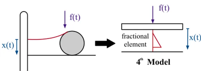
(2) Some recent works highlight a fractal structure of some soft materials [1, 8, 23, 18, 21]. Such a fractal structure consolidates the approach based on the use of a non-integer model to characterize its dynamic behaviour. A fractional model, due to its infinite dimension nature, is particularly adapted to model complex systems with few parameters and to obtain an adequate exploitable model [11]. Likewise, non-integer models play an important role in describing dynamical properties of linear viscoelastic systems, as in case of biological tissues (see e.g. [10, 19, 22, 12]) or mechanical systems in general [13]. However, to the best of the authors’ knowledge fractional identification methods have not been applied to soft materials in robotics applications.. x(t). b damper. K spring. x(t). nd. 2 Model. Figure 1: Scheme of the mechanical impedance of the environment: spring-damper model (Model 2). As mentioned, the mechanical impedance of the environment is typically modelled as a springdamper system. In this paper, four different models are considered to characterize it as follows.. Motivated by this context, this paper investigates how fractional calculus can help to model the mechanical impedance of the environment, and concretely soft objects, with which a flexible link contacts in order to be able to design robust control during the interaction. For this purpose, an experimental setup is built consisting of a flexible link, actuated by a motor, that interacts with a soft object. The force exerted on the object is measured by means of a load cell. A total of 50 experiments are carried out with ten different objects (five experiments per object). For each object, four different models are identified: 1) lineal regression model, 2) spring-damper model, 3) spring-damper model with a spring for the robotic arm, and 4) fractional order extension of springdamper model.. The first model (henceforth referred to as model 1) considers a mechanical impedance given by lineal behavior between the applied force –f (t)– to the object and its displacement –x(t)– owing to its deformation. Thus, the model can be expressed as: f (t) = a1 x(t) + a0 ,. (1). where a1 and a0 are constants. The second model (referred to as model 2) of the mechanical impedance is the well-known springdamper model: f (t) = K(x(t) − x(t0 )) + b. d(x(t) − x(t0 )) , dt. (2). where K and b are the stiffness and damping characteristic of the objects, being x(t0 ) = 0 the position of the impacted surface at the moment of the collision and which is the equilibrium position at which the object is not compressed and therefore f (t0 ) = 0, as shown in Fig. 1. The spring represents the elastic behavior, whereas the damper refers to the dynamics of the object to absorb the variation of displacement.. The remainder of this paper is organized as follows. The four models considered in this study are explained in Section 2. Experiments, identification method, and results are discussed in Section 3. Finally, conclusions and future works are drawn in Section 4.. 2. f(t). f(t). MODELS. In Laplace-domain, the model can be expressed as a transfer function as:. Let consider a single-link flexible arm which is displaced by a motor in vertical plane. This section describes the mechanical impedance of objects when the tip contacts with it (constrained motion).. 1/b X(s) = , F (s) s + K/b. For a better understanding of the problem to be studied, let us formulate the following hypothesis:. (3). The third model (model 3) do not only consider the dynamics of the environment, but also takes into account the elastic nature of the actuator – the load cell, in this case– that applies the force with its tip over the object (see Fig. 1). Thus, model (3) is redefined as:. a) Consider a link of negligible mass. b) The velocity of displacement of the link is slow. c) The mass of the load is quite a lot bigger than that of the bar.. K1 s + K1 K2 /b X(s) = , F (s) s + (K1 + K2 )/b. d) The arm is not affected by gravity.. 711. (4).

(3) The last model (referred to as model 4) assumes that the environment can be modelled as a fractional order mechanical impedance (see Fig. 3) given by. f(t) f(t). dα (x(t) − x(t0 )) , (5) f (t) = K(x(t) − x(t0 )) + b dtα. th. Figure 3: Scheme of the mechanical impedance of the environment: fractional generalization of spring-damper system (Model 4).. Table 1: Properties of the flexible link Material 301 SS. (6). EXPERIMENTS AND RESULTS. EXPERIMENTAL SETUP. x(t). Young’s modulus (N/m2 ) 2·1011. Density (kg/m2 ) 20389. Worm screw. f(t) K1. b damper K2 spring. Cross section inertia (m4 ) 2.33·10−11. Ten soft objects with different properties were selected in this study to be identified. Five different experiments were carried with each, resulting in a. The experimental platform consists of a flexible link actuated by a stepper motor through a worm screw. The base of the flexible link is attached. f(t). Width (mm) 7.925. The sensor to measure the force applied to the object is integrated by a couple of strain gauges which are cemented to both sides of the root of the link. The position is known indirectly through the excitation of the motor with a precision of 6.28 × 10−9 m. The electrical signal provided by the strain gauges is conditioned by a strain gauge amplifier and an analog-to-digital converter with 24-bit resolution. A microcontroller Atmel ATmega32u4 is used to govern the motor, read the signal of the gauges and communicate with a computer by USB. The system runs with a sampling time of Ts = 10 ms.. This section contains the description of the experimental setup used to obtain the measurements of the force applied to the object contacted and the flexible link. It also explains the identification method carried out to characterize the objects and the results. 3.1. Length (mm) 31.75. to the worm screw, which is attached itself to the output axis of the stepper motor which drives the system. The worm screw only allows vertical displacement. The stepper motor has a reduction relation of n = 18 90 . Figure 4 illustrates a scheme of the experimental setup. The physical characteristics of the flexible arm are given in Table 1.. The transfer function of model is:. 3. x(t). 4 Model. where α is the (unknown) parameter of the environment, which includes the possibility of viscoelastic and rheological effects. In this model, pure spring and damper behaviour can be obtained for α = 0 and α = 1, respectively (see e.g. [13]). Thus, the spring-damper behaviour corresponding to a traditional mechanical impedance can be represented when α = 1. It must be remarked that dynamics of actuator is neglected in this model owing to the actuator has a less elasticity in comparison with the softmaterials. To verified this assumption, the actuator was characterized and modeled as a spring. The carried out experiments –omitted for clarity purposes– allowed us to determine a stiffness of 3885.05 N/m, which is one, or even two, order of magnitude higher than that of the materials used.. 1/b X(s) = α . F (s) s + K/b. fractional element. x(t). Flexible link. Object. Strain Gage. x(t). rd. 3 Model. Motor. Figure 2: Scheme of the mechanical impedance of the environment: spring-damper model with a spring for the robotic arm (Model 3).. Figure 4: Configuration of the experimental setup.. 712.

(4) Table 2: Fitting results for the integer and fractional models for the objects impacted. Experiment Object 1 Object 2 Object 3 Object 4 Object 5 Object 6 Object 7 Object 8 Object 9 Object 10. Model 1 (given by (1)) a1 a0 154.65 −28.99 142.70 −25.31 62.80 −29.65 110.19 −29.31 77.02 −14.59 93.79 −19.75 140.03 −6.91 72.79 −23.64 88.90 −17.49 76.13 −11.64. Model 2 (given by (3)) 1/b K/b 752.4 3.81 975.9 6.17 85.71 7.76 × 10−1 340.90 2.28 363.7 4.27 460.00 4.30 6809.00 48.49 208.7 2.35 512.40 5.27 752.00 9.62. Model 3 (given by (4)) K1 K1 K2 /b (K1 + K2 )/b 68.32 218.30 0.52 92.66 78.75 1.93 × 10−12 49.4 1299.00 23.58 74.64 81.21 0.3076 72.54 82.98 4404.00 59.65 17.02 4.10 × 10−8 127.30 19.62 1.30 × 10−12 37.95 31.82 2.99 × 10−6 58.24 43.32 1.09 × 10−1 77.72 5224.00 72.51. Model 4 (given by (6)) 1/b K/b α 176.61 6.15 × 10−12 0.35 150.07 1.77 × 10−1 0.25 52.49 3.24 × 10−13 0.44 112.55 1.08 × 10−11 0.37 72.54 1.52 × 10−13 0.19 93.18 1.10 × 10−11 0.25 140.83 7.26 × 10−13 0.04 66.45 2.63 × 10−12 0.31 86.71 9.92 × 10−11 0.21 73.16 2.12 × 10−12 0.13. Table 3: Performance indices for the integer and fractional models for the objects impacted. Experiment Object 1 Object 2 Object 3 Object 4 Object 5 Object 6 Object 7 Object 8 Object 9 Object 10. MSE 221.00 115.95 313.13 249.76 150.63 105.12 17.76 143.63 73.81 45.61. Model MAD 12.70 9.15 14.89 14.14 10.59 8.60 3.24 10.28 6.93 5.58. 1 (given R2 0.9812 0.9907 0.9699 0.9787 0.9871 0.9882 0.9986 0.9850 0.9920 0.9951. by (1)) AIC w (%) 624.90 0 617.25 0 1526.90 0 892.88 0 1162.50 0 776.82 0 383.82 0 1101.80 0 769.73 0 806.31 0. MSE 81.56 44.92 176.63 110.97 137.18 54.62 19.35 62.39 38.80 38.21. Model MAD 6.84 5.57 10.34 9.01 10.40 6.22 3.40 6.54 5.21 5.40. 2 (given R2 0.9931 0.9964 0.9830 0.9905 0.9883 0.9939 0.9984 0.9935 0.9958 0.9959. by (3)) AIC w (%) 510.26 0 494.93 0 1375.20 0 762.27 0 1140.90 0 668.15 0 395.15 0 917.55 0 655.26 0 769.10 0. total of fifty different experiments. Both the force applied to the object and the displacement of the flexible link due to its deformation were measured in each experiment. For that purpose, the motor is stimulated with a lineal velocity of 518 µm/s until a force of 500 gf –4.90 N– is reached (the experiment stops at that moment). It is important to remark that, a test protocol was established to guarantee the repeatability, reproducibility and comparability of the results. 3.2. ,. w (%) 100 0 0 0 0 0 88.69 100 100 0. MAD =. Model MAD 4.98 3.33 6.78 5.34 7.25 3.77 2.71 3.55 2.64 3.37. MSE 35.49 16.89 57.06 39.96 64.45 20.43 12.66 16.74 11.65 16.43. 4 (given R2 0.9970 0.9986 0.9945 0.9966 0.9945 0.9977 0.9990 0.9983 0.9987 0.9982. by (6)) AIC 416.68 370.88 1077.80 599.92 968.44 507.01 341.27 628.81 443.16 594.00. w (%) 0 100 100 100 100 100 11.31 0 0 100. |yj − ŷj |. j=1. N. .. (8). 2. The coefficient of determination (R2 ∈ (0, 1)), given by N P 2. R =1−. (yj − ŷj )2. j=1 N P. , (yj −. (9). ȳ)2. j=1. where ȳ is the mean of the real measurements. 3. The Akaike information criterion (AIC) [2]: N X. 2. (yj − ŷj ). 2K(K + 1) , N −K −1 (10) being K the number of parameters of the model. The value of the AIC does not give information about the quality of a model. However, comparing the AIC values of different models, it can be seen which ones are more likely to be a good model for the data, as a lower value indicates a more likely model. Furthermore, if there are M models,. AIC = N log. (yj − ŷj )2 N. by (4)) AIC 375.33 421.59 1666.90 941.53 1238.20 1149.50 337.15 484.11 310.88 928.23. N P. The fitting procedure was implemented in MATLAB. The parameters of models (1), (3) and (4) were estimated through linear regression of their corresponding time-domain responses based on a least-squares fit. To estimate the parameters of fractional model (6), an iterative process was used based on least-squares fit: the fractional coefficient was calculated by Nelder-Mead’s simplex search method (implemented in the function fminsearch) minimizing the mean square error (MSE), given by. MSE =. 3 (given R2 0.9979 0.9980 0.9494 0.9716 0.9823 0.8904 0.9990 0.9991 0.9994 0.9914. 1. The mean absolute deviation (MAD), given by. In order to determine what of the integer and fractional models proposed characterizes better the object impacted, an identification procedure was developed to determine the parameters ai , bi , and α of the models as follows.. j=1. Model MAD 4.11 3.89 19.70 16.13 11.83 22.97 2.78 2.70 1.94 7.78. to evaluate the quality of the fit obtained by the resulting models: other performance indices were calculated as well. These were:. IDENTIFICATION METHOD. N P. MSE 24.77 25.03 526.98 333.55 207.18 980.09 12.27 8.70 5.54 80.72. (7). where N is the number of points, and yj and ŷj are the real measurement and the model output, respectively. The MSE alone is not relied upon. 713. j=1. N. +2K+.

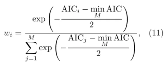
(5) the Akaike weight, given by AICi − min AIC M. exp − wi =. M X. for the robotic arm, and 4) fractional order extension of spring-damper model. ! The experimental data (a total of 50 experiments with 10 different objects) was used to identify the unknown parameters of the models. The goodness of the adjustment were analyzed by a set of performance indices. The results showed that fractional models had better performance in most cases in comparison with the classical alternatives proposed in the literature.. 2 AICj − min AIC. exp −. j=1. ! , (11). M. 2. provides the probability of model i being the best of all the M models.. Our future work will include: 1) the design of robust controllers for this problem, and 2) the study of contacts at any point of the link.. It is important to remark: 1. For the identification, the average of the five experiments carried out for each object were used.. ACKNOWLEDGMENT. 2. The function fotf [14] was used in the identification process to obtain the time-domain response of the fractional models. 3.3. This work has been supported by the Spanish Ministry of Economy and Competitiveness under the project with reference DPI2016-80547-R.. RESULTS. References. Figure 5 shows the fitting results obtained for the ten objects. The experimental data demonstrates a different behaviour between objects and, consequently, allows us to identify different grades of soft materials. The plots also show that the responses of the proposed models, where it can be seen that models 1 and 2 are not able to describe the system dynamics: the values obtained for the MSE are high. In contrast, the models 3 and 4 achieve the best fitting to experimental data as will be described next.. [1] S. Aime, L. Cipelletti, and L. Ramos. Power law viscoelasticity of a fractal colloidal gel. Submitted to Condensed Matter Physics, 2018. [2] H. Akaike. A new look at the statistical model identification. IEEE Transactions on Automatic Control, 19(6):716–723, 1974. [3] M. Benosman and G. Le Vey. Control of flexible manipulators: A survey. Robotica, 22(5):533–545, 2004.. The estimated parameters for the four models for all the objects are given in Table 2, whereas Table 3 includes the performance indices of the models identified (the best results are in bold). According to Table 3, it can stated that fractional model (6) achieves a better adjustment to experimental data (in particular, for six of the ten objects). Consequently, fractional model (6) may characterize successfully the dynamics of the impact of a flexible link with soft objects. However, it should be said that model (4) also performs a good adjustment in some cases.. 4. [4] Hadi Delavari, Patrick Lanusse, and Jocelyn Sabatier. Fractional order controller design for a flexible link manipulator robot. Asian Journal of Control, 15(3):783–795, 2013. [5] Vicente Feliu, Blas M. Vinagre, and Concepción A. Monje. Advances in Fractional Calculus, chapter Fractional-order Control of a Flexible Manipulator, pages 449–462. Springer, 2007. [6] Vicente Feliu-Batlle. Robot flexibles: Hacia una generación de robots con nuevas prestaciones. Revista Iberoamericana de Automática e Informática Industrial, 3:24–41, 2006. (In Spanish).. CONCLUSIONS. This paper has focused on modelling the mechanical impedance of the environment contacted by a flexible link based on the well-known springdamper system, but considering models of both integer and fractional order. In particular, four models were identified for a group of soft objects: 1) linear regression model, 2) spring-damper model, 3) spring-damper model that also includes a spring. [7] Daniel Feliu-Talegón, Vicente Feliu-Batlle, Blas M. Vinagre, Inés Tejado, and Hassan HosseinNia. Stable force control and contact transition of a single link flexible robot using a fractional-order controller. Submitted to ISA Transactions, 2018.. 714.

(6) 2.5 2 1.5. 3 Experimental data Model 1 (R2 = 0.9812). 2.5. Model 2 (R2 = 0.9931). 2. Model 3 (R2 = 0.9979) 2. Model 4 (R = 0.997). 1.5. Experimental data Model 1 (R2 = 0.9907) Model 2 (R2 = 0.9964) Model 3 (R2 = 0.998) Model 4 (R2 = 0.9986). 1 1 0.5. 0.5. 0 -100. 0. 100. 200. 300. 3.5. 6 5. 3. Model 3 (R2 = 0.9494). 0. 3. Experimental data Model 1 (R2 = 0.9787). 2.5. Model 2 (R2 = 0.9905). Experimental data Model 1 (R2 = 0.9699) Model 2 (R2 = 0.983). 4. 0 -100. 400. 2. Model 4 (R2 = 0.9945). 100. 200. 300. 400. 100. 200. 300. 400. Model 3 (R2 = 0.9716) Model 4 (R2 = 0.9966). 1.5 2. 1. 1. 0.5. 0 -100. 0. 100. 200. 300. 3. 0. 3.5. 5 4. 0 -100. 400. Experimental data Model 1 (R2 = 0.9871). 3. Experimental data Model 1 (R2 = 0.9882). 2.5. Model 2 (R2 = 0.9939). 2. Model 2 (R = 0.9883) Model 3 (R2 = 0.9823). 2. Model 4 (R2 = 0.9945). Model 3 (R2 = 0.8904) Model 4 (R2 = 0.9977). 1.5. 2. 1 1. 0.5. 0 -100. 3 2.5. 0. 100. 200. 300. 0 -50. 400. 1.5. 50. 100. 150. 200. 250. 300. 350. 100. 150. 200. 250. 300. 350. 100. 150. 200. 250. 300. 350. 5. Experimental data Model 1 (R2 = 0.9986). 4. 2. Model 2 (R = 0.9984). 2. 0. Model 3 (R2 = 0.999). 3. Model 4 (R2 = 0.999). Experimental data Model 1 (R2 = 0.985) Model 2 (R2 = 0.9935) Model 3 (R2 = 0.9991) Model 4 (R2 = 0.9983). 2 1 1. 0.5 0 -100. 0. 100. 200. 300. 0 -50. 400. 4. 4. Model 2 (R2 = 0.9958) 2. Model 3 (R = 0.9994). 2. 50. 5 Experimental data Model 1 (R2 = 0.992). 3. 0. 3. Model 4 (R2 = 0.9987). Experimental data Model 1 (R2 = 0.9951) Model 2 (R2 = 0.9959) Model 3 (R2 = 0.9914) Model 4 (R2 = 0.9982). 2 1. 0 -50. 1. 0. 50. 100. 150. 200. 250. 300. 0 -50. 350. 0. 50. Figure 5: Fitting results for the impact with ten soft objects. [8] Jianying Hu, Yu Zhou, Zishun Liu, and Teng Yong Ng. Pattern switching in soft cellular structures and hydrogel-elastomer composite materials under compression. Polymers, 9(6):229, 2017.. [9] O.D. Cortázar I. Payo, V. Feliu. Force control of a very lightweight single-link flexible arm based in coupling torque feedback. Mechatronics, (19):334–347, 2009. [10] C. Ionescu, A. Lopes, D. Copot, J. A. T.. 715.

(7) Machado, and J. H. T. Bates. The role of fractional calculus in modeling biological phenomena: A review. Communications in Nonlinear Science and Numerical Simulation, 51:141–159, 2017.. [22] Zoran B. Vosika, Goran M. Lazovic, Gradimir N. Misevic, and Jovana B. SimicKrstic. Fractional calculus model of electrical impedance applied to human skin. PLoS One, 8(4):e59483, 2013.. [11] Richard L. Magin. Fractional calculus in bioengineering. Begell House, 2004.. [23] R. Y. Wang, P. Wanga, J. L. Li, B. Yuan, Y. Liu, L. Li, and X. Y. Liu. From kineticstructure analysis to engineering crystalline fiber networks in soft materials. Physical Chemistry Chemical Physics, 15(9):3313– 3319, 2013.. [12] Richard L. Magin. Fractional calculus models of complex dynamics in biological tissues. Computers & Mathematics with Applications, 59(5):1586–1593, 2010. [13] Francesco Mainardi. Fractional Calculus and Waves in Linear Viscoeslasticity. An Introduction to Mathematical Models. Imperial College Press, 2010.. c 2018 by the authors. Submitted for possible open access publication under the terms and conditions of the Creative Commons Attribution CC-BY-NC 3.0 license (http://creativecommons.org/licenses/by-nc/3.0/).. [14] C. A. Monje, Y. Q. Chen, B. M. Vinagre, D. Xue, and V. Feliu. Fractional-order Systems and Controls. Fundamentals and Applications. Springer, 2010. [15] A. Mujumdar, S. Kurode, and B. Tamhane. Fractional order sliding mode control for single link flexible manipulator. In Proceedings of the 2013 IEEE International Conference on Control Applications (CCA’2013), pages 288–293, 2013. [16] A. Mujumdar, B. Tamhane, and S. Kurode. Fractional order modeling and control of a flexible manipulator using sliding modes. In Proceedings of the 2014 American Control Conference (ACC’14), pages 2011–2016, 2014. [17] E. Pereira, J. Becedas, I. Payo, F. Ramos, and V. Feliu. Robot Manipulators Trends and Development, chapter Control of Flexible Manipulators. Theory and Practice, pages 1– 31. In Tech, 2010. ISBN: 978-953-307-073-5. [18] M. Takenaka. Analyses of hierarchal structures of soft materials by using combined scattering methods. Nippon Gomu Kyokaishi, 1:7–13, 2011. [19] Inés Tejado, Duarte Valério, Pedro Pires, and Jorge Martins. Fractional order human arm dynamics with variability analyses. Mechatronics, 23:805–812, 2013. [20] M. O. Tokhi and A. K. M. Azad, editors. Flexible Robot Manipulators. Modelling, simulation and control. The Institution of Engineering and Technology, 2008. [21] Kaoru Tsujii. Fractal materials and their functional properties. Polymer Journal, 40:785–799, 2008.. 716.

(8)