TítuloVascular damage detection through deep learning

(1)

Facultade de Informática

TRABALLO FIN DE GRAO GRAO EN ENXEÑARÍA INFORMÁTICA

MENCIÓN EN COMPUTACIÓN

Vascular damage detection through

deep learning

Estudante: Ángel Rodríguez Martínez

Dirección: Manuel Francisco González Penedo Víctor Manuel Mondéjar Guerra Lucía Ramos García

(2)

(3)

(4)

(5)

Acknowledgements

First of all I would like to thank my tutors Lucía, Víctor and Manuel for guiding me and helping me developing this project, their cheerfulness and passion for what they do was an invaluable source of motivation for me. Another big part of the knowledge and help I needed for this project came from my colleague Mateo. Finally I would like to thank the University of A Coruña for giving me a fantastic education and a lot of great moments to remember.

(6)

(7)

Abstract

HET-CAM (Hen’s Egg Test - ChorioAllantoic Membrane) is a type of pharmaceutical analysis that measures the toxicity of a solution by administrating it to the chorioallantoic membrane of a fertilised egg. The membrane is used as an analogous tissue to that of the human eye in order to determine if a substance is suitable for human use. The process is recorded in video and analysed to chronologically locate three phases (haemorrhage, lysis and coagulation) that allow the classification of the toxic potential of the substance. HET-CAM is frequently used in the pharmaceutical industry to test substances, especially those destined to be used on the human eye. This approach has several advantages with respect to other methods like the Draize Test. It is easy to perform, affordable, and prevents unnecessary animal suffering. The main disadvantage is that the process is tedious and can be subjective as the beginning of each phase is manually marked by the person performing the analysis.

This project aims to use computer science techniques, specifically deep learning and im-age processing, to automatically analyse the videos and set a more reliable ground for the classification of the substances. These techniques applied to the HET-CAM videos allow the extraction of objective data that defines the processes taking place in the membrane. This data can then be studied by the system to make an initial classification of the substance which can then be used by experts to make a more informed decision.

Since there are no bibliographic precedents on solving this problem using artificial intel-ligence, part of the project will consist on the creation of a dataset that suits the needs of the chosen network architecture.

Resumen

(8)

Este proyecto pretende usar técnicas de computación, especialmente deep learning y pro-cesado de imagen, para analizar automáticamente los vídeos y sentar una base más sólida a la hora de clasificar las sustancias. Estas técnicas aplicadas a los vídeos HET-CAM permiten la extracción de datos objetivos que definan los procesos que están teniendo lugar en la mem-brana. Estos datos son estudiados por el sistema para hacer una clasificación inicial que los expertos pueden usar para tomar decisiones más informadas.

Dado que no hay antecedentes bibliográficos resolviendo este problema usando inteli-gencia artificial, parte del proyecto consistirá en la creación de un conjunto de datos que se amolde a las necesidades de la arquitectura de red escogida

(9)

(10)

(11)

Contents

3.4 Bleeding evolution module . . . 31

4 Software Development 43 4.1 Image extraction and pre-processing. . . 43

4.1.1 Design . . . 44

4.1.2 Implementation . . . 45

4.2 Image marker . . . 46

4.2.1 Implementation . . . 47

4.2.2 User guide . . . 49

5 Results 53 5.1 Detection of bleeding in HET-CAM videos . . . 53

5.2 Evolution of bleeding in HET-CAM videos . . . 55

5.3 Potential and constraints . . . 57

6 Conclusion and future work 61 6.1 Conclusion . . . 61

6.2 Future work . . . 63

A Project planning 67

List of Acronyms 69

Glossary 71

(12)

List of Figures

2.1 The steps of the HET-CAM test. . . 6

2.2 Four different frames corresponding to the stages of the irritation process given by an expert . . . 7

3.4 Exhaustive marking (154 marks) vs. ignoring too small haemorrhages (42 marks) 16 3.5 Blurry haemorrhages that were not annotated . . . 17

3.13 Example of model detecting more haemorrhages than the annotated by the dataset . . . 38

3.14 Example of a random transformation in the HSV colour space following the stated parameters . . . 38

3.15 Data augmentation experiments’ training metrics . . . 39

3.16 Data augmentation experiments’ validation metrics . . . 40

3.17 Fold 1 test results of a frame: TP(green), FP(red), FN(blue). . . 41

3.18 Evolution of bleeding in different frames: TP(green), FP(red), FN(blue). . . 41

(13)

List of Figures

4.1 Aspect ratio converter: Input image - Left sub-image - Right sub-image . . . . 45

4.2 Image Marker use case diagram . . . 46

4.3 State Pattern class diagram . . . 48

4.4 Image Marker class diagram . . . 48

4.5 User interface of the Image Marker script . . . 51

4.6 Open file dialog window . . . 52

5.1 Detection in three equispaced frames in video DSC_1104 . . . 53

5.2 Detection in three equispaced frames in video DSC_1107 . . . 54

5.3 Blurry haemorrhages not detected towards the end of DSC_1104 . . . 54

5.4 Evolution of haemorrhage in positive and negative videos . . . 55

5.5 Timing of the experts in several analysed videos . . . 59

A.1 Initial project planning schedule, divided into tasks . . . 68

(14)

List of Tables

3.1 Source data specification . . . 14

3.2 A data tag sample . . . 14

3.3 Final state of the dataset . . . 17

3.4 Confusion matrix values . . . 19

3.5 5-fold cross-validation structure . . . 21

3.6 Final configuration’s best epoch test metrics . . . 30

4.1 Specification ofFrameExtractor.py . . . 44

4.2 Specification ofAspectRatioConverter.py. . . 44

4.3 Image Marker key-bindings. . . 50

(15)

(16)

Chapter 1

Introduction

Information Technologies (IT) are used in almost every part of the world to help humans solve complex problems in a fast and easy manner. One of the branches of IT is Artificial Intelligence (AI) which, as a broad description, is used to make a computer ”think in a human-like fashion”. This is very useful for solving problems that are not very well defined and therefore cannot be solved using an algorithmic approach, usually classification or regression problems.

1.1 Problem Description

In the pharmaceutical industry, several parameters need to be tested before releasing a drug to the market to ensure that it is suitable for human consumption. One of these parameters is the toxicity, which measures the potential ability of the drug to cause damage to human tissue. In the case of products destined to be used in the eyes, various tests exist, like the Draize Test[1] or the Hen’s Egg Test - ChorioAllantoic Membrane (HET-CAM)[2]. The latter is the one that is going to be analysed in this study.

(17)

1.2. Motivation

1.2 Motivation

The main drawback of HET-CAM is its low repeatability, mainly due to a subjective apprecia-tion of the occurrence of reacapprecia-tions caused by the irritating substances, the differences among experts and the variability of the chorioallantoic membrane. Besides the subjectivity, the manual characterisation of the haemorrhage, lysis and coagulation timings is a tedious and time-consuming task. The nature of the HET-CAM procedure allows recording video footage of the process to analyse it at a later time. The motivation of this project is the automation of the assessment of that video footage in order to reduce the subjective character of the HET-CAM test allowing a reliable and repeatable extraction of objective data that supports the experts’ decisions regarding the toxicity of the substance.

A previous study conducted by Gende [3] explores the use of computer vision techniques for extracting objective data from HET-CAM videos in terms of the amount of blood and blood vessels at each frame of the sequence. A big part of the project was dedicated to define the features needed to be analysed in order to get the wanted output. In this case, the areas of interest were the blood vessels and the ramifications where haemorrhages occur. To detect those areas using an algorithmic approach it was necessary to iteratively apply filters that accentuate the features and erase background and noise until valid outputs are obtained. The results extracted from this study shows that classical computer vision approaches allows to extract useful data from HET-CAM videos, however, in addition to the need of manually defining the relevant features to analyse, these techniques are affected by the variety of the data, the lighting conditions and are quite sensitive to parameter tuning.

In recent years, Deep Learning (DL) techniques have arisen as a promising alternative to address object detection problems given its ability to recognise complex patterns from raw input data, learning proper hierarchical representations of the underlying information at different levels. In the context of HET-CAM test, the project would be considered as an object recognition problem where the haemorrhage areas in each frame need to be detected.

Therefore, in this work, it is proposed the use of DL techniques for extracting objective information from HET-CAM videos. By solving this problem using DL a more robust system can be created, being less vulnerable to noise, colour or illumination changes, and supporting multiple resolutions. Making the program support all kinds of videos will also promote the use of HET-CAM in otherwise reluctant laboratories.

1.3 Objectives

(18)

CHAPTER 1. INTRODUCTION

that show the evolution of bleeding areas) and displays it in a way that helps experts make a decision on the toxicity of the drug. To accomplish this objective, the system will look at the videos as an image recognition problem. The system will analyse the videos frame by frame detecting each area of bleeding, then the output will be constructed using this information. The complete problem was divided into several sub-objectives that need to be achieved.

• Create a dataset: A dataset is the collection of tagged data used to train and validate AI systems. Since there is not bibliography in using AI systems to analyse HET-CAM videos, a custom dataset needs to be created from the videos that are available. A pro-gram will be developed to aid in the transformation of the raw data into an annotated dataset.

• Train several network configurations: Several parameters and configuration op-tions can be changed in AI systems. The consequences of changing this factors will be studied in order to achieve the most appropriate configuration. Some of the parameters that are going to be considered are: variations on the learning rate, use of pretrained models or data augmentation.

• Compare the results with experts’ annotations: Finally, once the appropriate sys-tem configuration is chosen, the data extracted from the videos will be compared with the annotations made by the experts to see how they are correlated.

1.4 Outline

This document is split into 6 different chapters to help the reader understand the problem, the methodology followed and the outcomes. The planning and time scheduling of the process are detailed in AppendixA.

• Chapter1: IntroductionThis chapter provides an introduction to the problem, de-tailing its description, the motivation behind the work, and the objectives that need to be accomplished.

• Chapter2: Domain descriptionThis chapter contains an explanation of the domain of the problem, including a more detailed description of the HET-CAM test, as well as the information needed to implement the artificial intelligence network.

(19)

1.4. Outline

help with the annotation procedure. Then, the bleeding detection module is described, including the extensive process for the parameter adjustment. Finally, the bleeding evolution module that allows generating informative graphs for the HET-CAM videos is presented.

• Chapter4: Software developmentThis chapter provides a detailed view of the design and implementation of the different software tools developed and used throughout the project.

• Chapter5: ResultsThis chapter presents the results provided by the proposed method-ology regarding the bleeding detection and the bleeding evolution throughout the HET-CAM videos, assessing the distinction between negative and positive videos, as well as the relation with the experts’ timings. Additionally, the extracted results are discussed, highlighting the potential and constraints of the methodology.

(20)

Chapter 2

Domain description

This project consist on the implementation of an IT system, specifically Deep Learning, to be used in the pharmaceutical industry to serve as support for the experts when analysing the toxicity of drugs via the HET-CAM test. In this chapter, all preliminary knowledge needed on HET-CAM and Deep Learnig will be presented.

2.1 HET-CAM

The toxicity of a drug is the potential it has to harm live tissue. Toxicity testing is a part of the preclinical testing phase in the development cycle of a drug and it must be done before studies on humans can begin in order to avoid unnecessary damage. HET-CAM is the acronym for Hen’s Egg Test - ChorioAllantoic Membrane and it is a procedure to where the membrane of a hen’s egg is used to test the drug because of its similar vascular structure to the human eye. The drug is applied and the reactions taking place in the membrane are observed to determine the toxicity score of the substance. HET-CAM was found to return similar results to the Draize test [4] with the advantage that it is not performed over live animals.

To start the procedure, the egg needs to be fertilised for 9 days. Then the egg is placed on a stand and an opening is cut in the outer shell using a saw. Then the outer most membrane is retired, leaving the CAM visible. Now the egg is ready for the test. It is placed below the recording device of choice and the solution to be tested is applied to the membrane using a pipette. The reactions taking place in the membrane are recorded for 5 minutes, then the test is considered complete. The whole procedure is summarised in figure2.1(page6).

(21)

2.1. HET-CAM

Figure 2.1: The steps of the HET-CAM test

solidification of the blood outside blood vessels. The timing of these three stages determines how irritant a drug is. A visual differentiation between stages can be observed in figure2.2 (page7)

The toxicity of the drug is represented by the so-called Irritation Score (IS). It is calcu-lated using the time at which these three stages occur. The following formula relates the haemorrhage timeTH, lysis timeTLand coagulation timeTC with the irritation score [4].

IS=

(22)

CHAPTER 2. DOMAIN DESCRIPTION

Figure 2.2: Four different frames corresponding to the stages of the irritation process given by an expert

2.2 Deep learning

During the last decade, Deep Learning has demonstrated to be an excellent technique in the area of artificial intelligence, solving different problems, and even surpassing humans in some cases [5,6]. In addition, DL yields good results in diverse areas like image recognition [7], medical imaging [8], or speech recognition [9].

(23)

com-2.2. Deep learning

plex patterns directly from the raw data, learning proper hierarchical representations of the underlying information at different levels. Therefore, DL methods are able to perform both tasks (the representation of the data and the classification) at the same time just by feeding the network with raw data [5].

This feature of DL makes it a good candidate for object recognition problems. Being able to train the network in a set of images whose desired output is known can save a lot of time and return better results in comparison to trying to detect the objects via computer vision tech-niques. A well known object detection algorithm based on artificial intelligence, designed by Girshick et al.[10], mixes Convolutional Neural Networks (CNN) with a concept called region proposals. The performance of this system showed a large increase in performance compared to other methods. Since then, object recognition using CNNs has seen lots of de-velopments [11][12][13][14], which points to this type of system being the appropriate one for the problem at hand.

The problem with object detectors like R-CNN [10] is that the require a good amount of pre-processing of the images and use other complex algorithms to filter the output. Optimis-ing a model like this to a specific problem requires a lot of fine tunOptimis-ing, since the different parts of the model are optimised separately. An alternative method of object detection using deep learning is the You Only Look Once (YOLO) model [13]. This model encapsulates the whole procedure in a single CNN, taking as inputs the raw images and giving bounding boxes of objects as outputs.

In the specific context of this project, the YOLO architecture has been previously used to address the detection of structures with morphological characteristics similar to the haemor-rhages produced in HET-CAM videos, such as the detection of carcinogenic masses in mam-mography images [15] or the detection of lung nodules in computed tomography scans [16]. The results achieved in these proposals serve as a precedent to promote the use of the YOLO architecture for detecting the bleeding areas in HET-CAM videos.

2.2.1 You Only Look Once (YOLO)

(24)

CHAPTER 2. DOMAIN DESCRIPTION

confidence are the output of the network. Finally, non maximum suppression is applied to the outputs to erase detections with less than a confidence threshold. The process is graphically represented in figure2.3(page9).

Figure 2.3: Simple explanation of the YOLO object recognition system

The architecture of the neural network (Figure 2.4, page9) is comprised of 24 convolu-tional layers followed by 2 fully connected layers. The final layer of the network calculates the bounding boxes as well as the class probabilities. Bounding boxes are normalised between 0 and 1.

Figure 2.4: YOLO network architecture

The loss function that is optimised during training is composed of a series of factors that are then summed to get the total loss.

• Bounding box location and dimensions:The mean squared error is used to calculate the difference between each detection and its ground truth counterpart.

(25)

2.2. Deep learning

• Confidence loss:It also uses the binary cross entropy formula. This term is calculated for each grid cell if it is responsible for a detection and it computes the class confidence of that cell compared with the ground truth class value for that cell.

The confidence loss can be driven towards 0 by the cells that do not count with any object. Taking this into account, two factors are introduced in the formula to balance the weight confidence loss and bounding box loss. For a more detailed view on the loss formula and more specific details of the model, the reader can refer to reference [13].

(26)

Chapter 3

Methodology

The steps taken to solve the problem will be specified in this chapter. First, an outline of each step will be presented, lightly detailing what needs to be done. The following sections will tackle the concrete analysis, implementation and result of each step.

3.1 Methodology outline

In order to analyse the videos and automatically gather valuable information from them, an application will be developed that uses a deep learning network to find the areas of interest. This structure will be used to locate the areas of bleeding in each frame to later on print graphs that represent the evolution of the bleeding area with respect to the time in the videos. The proposed methodology to analyse the HET-CAM videos is the following, as it can be seen in figure3.1(page12):

• Capturing video frames:in fixed size batches to be passed to the deep learning system for their analysis. Some pre-processing might be needed, such as re-scaling each frame to a fixed resolution or skipping a number of frames between samples.

• Analysing the frames using object detection via deep learning: The data from the previous step is passed to the artificial intelligence system to extract valuable in-formation from each frame, i.e. the areas detected as bleeding and their position and size.

• Building informative graphs:using the information gathered by the network for the experts to make decisions on the toxicity of the substance.

(27)

3.2. Dataset

Figure 3.1: Methodology outline diagram

near real time video. This second characteristic is not crucial for the concrete implementa-tion detailed in this document, but analysing a real time video feed (instead of pre-recorded videos) can be a feasible point of extension for future work in the program. YOLO was also chosen for its low number of background errors compared to other algorithms [13], since the area occupied by the objects is going to be measured, detecting part of the background as a haemorrhage is not desirable.

The network needs to be trained properly in order to be as robust and generalist as it can be. For the training process, the following steps need to be accomplished

• Build a dataset: since there is no bibliography on applying artificial intelligence to HET-CAM, there are no datasets available either. Building a dataset following the YOLO specification from the available videos will be the first step of the project.

• Train several network configurations:Various parameters need to be tested in order to obtain the network that best fits the problem. Experiments will be conducted altering these parameters and performance metrics will be recorded in order to pick the most appropriate model.

• Choose the most appropriate configuration: The results of the training (confusion matrices and other metrics) will be studied to pick the configuration that best fits the problem.

Finally, an application that uses the trained model to show the evolution of the bleeding areas of videos will be developed. The output of the program will then be compared to the times given by the experts in order to find if the information extracted by the network is useful in helping experts decide on the toxicity of a drug.

3.2 Dataset

(28)

CHAPTER 3. METHODOLOGY

of tagged data is needed so the system can learn which features are important in a certain context. Some examples of datasets are NMIST[17] which contains thousand of pictures of handwritten numbers, or ImageNet[18] which is a database of images of objects of all sorts.

In the context of this project, a dataset comprised of the different bleeding areas in HET-CAM videos is needed. No dataset tackling this concrete context was found so the creation of one was required. This section’s focus is to specify everything concerning the dataset: the source of the data, how it was annotated, and the limitations and problems that might be related with it.

3.2.1 Video data available

The videos used to build the dataset were recorded by experts of the Pharmacy Faculty of the University of Santiago de Compostela (USC) in December 2017. In the videos provided, both positive and negative test are performed on the same egg, one after the other. The negative control corresponds to a solution of sodium chloride (NaCl) and the positive corresponds to a solution of sodium hydroxide(NaOH). In the negative test no change in the membrane is seen during the whole length of the video. However, in the positive test, little accumulations of blood begin to appear around the blood vessels as the time passes, as seen in figure 3.2 (page13). The dataset will be comprised of images corresponding to different frames of each video, where the centre and size of the haemorrhage spots will be annotated.

Figure 3.2: Positive and negative frames

The data available consists in 18 HET-CAM videos corresponding to 7 different test eggs with a negative and a positive test in each egg. Most of the videos are around 5 minutes in length and there are recordings in three different resolutions across two aspect ratios (16:9, and 4:3). The specification of the data can be seen in table3.1.

(29)

3.2. Dataset

Egg Resolution Quality Filename Solution

1 1920x1080, 50p High DSC_1087 Nothing

1 1920x1080, 50p High DSC_1088 NaCl

1 1920x1080, 50p High DSC_1089 NaOH 0.1 N

2 1920x1080, 50p High DSC_1091 NaCl

2 1920x1080, 50p High DSC_1092 NaOH 0.1 N

3 1920x1080, 50p High DSC_1094 NaOH 0.1 N

4 1280x720, 50p High DSC_1097 NaCl

4 1280x720, 50p High DSC_1098 NaOH 0.1 N

5 640x424, 25p Low DSC_1099 Nothing

5 640x424, 25p Low DSC_1104 NaOH 0.1 N

6 640x424, 25p Low DSC_1106 NaCl

6 640x424, 25p Low DSC_1107 NaOH 0.1 N

7 640x424, 25p Low DSC_1109 NaOH 0.1 N

Table 3.1: Source data specification

measure was taken in order not to include a lot of copies of the same haemorrhage point, since they evolve slowly.

For the negative tests, a set of 10 representative frames were selected in order to cover the contrast and illumination variability of the HET-CAM videos. Since negative controls do not cause bleeding areas, manual marking of these frames is not needed.

3.2.2 Data tag specification

The different haemorrhages that comprises the dataset were annotated by a bounding box, which is delimited by the centre point(x, y), its width and height. Each image in the dataset must be accompanied by a.txtfile with the same name as the image where each line represents the bounding box of an object. Table3.2describes the structure of each line in the file.

Class index Centre_X Centre_Y Width Height

Table 3.2: A data tag sample

(30)

TheCentre_XandCentre_Y specify the position of the centre of the object andWidthand Heightrepresent its dimensions, all of them bounded between 0 and 1 with respect to the size of the image.

3.2.3 Data selection

A series of programs were developed to carry out the extraction of images from the videos and the later annotation of each of the selected frames. The development process of these tools is detailed in chapter4. But not all the frames in the videos are going to be annotated and included in the dataset. This sections objective is to explain the process that was followed to go from the raw video data, to the series of images that are going to be annotated in terms of their haemorrhage spots.

As it was stated in section3.2.1, from the 7 positive videos available only 5 were annotated by the experts in terms of the haemorrhage, lysis and coagulation times. These where the 5 videos used to conform the dataset.

Using the scripts mentioned in section4.1, image samples were taken from each video. The haemorrhage growth rate is slow at the beginning and is almost none at the end of the videos, therefore the amount of frames skipped between samples was set to 240, in order not to include a lot of duplicates of each haemorrhage point. It was observed that around the one minute mark, the variation of haemorrhage spots (even 240 frames apart) was almost negligible. There is a point in each video were the bleeding stops evolving and just becomes distorted and blurry, when different areas begin to merge and form big clots that occupy a large portion the picture. At this point the images were no longer included in the dataset. Therefore, only the first 10 images from each video were selected.

From the images selected, the ones that had a 16:9 aspect ratio were converted to 4:3. To avoid having duplicated haemorrhage areas in the dataset due to the overlapping region of the sub-images, just the most representative side was chosen to form part of the dataset.

3.2.4 Marking process

(31)

3.2. Dataset

Figure 3.3: Healthy blood vessel - Haemorrhage - Marked haemorrhage

With this in mind, the marking process began with the higher resolution videos. An ex-haustive search of the bleeding areas was performed, accumulating over 100 marks per frame (excluding the first frames in the videos, where the haemorrhage only recently started). Just in the first video (DSC-1089), which was HD converted to 4:3 aspect ratio (1440x1080 resolution), 1140 bleeding spots were marked. However, when proceeding to mark the lower resolution videos, like DSC-1104, it was found that the smaller bleeding areas that were marked in the previous (higher quality) video were barely recognisable, being regions of less than 100pixel2

(10x10pxarea). In order to preserve the marking process coherent between the videos, a low

bound was set on the size of the area of the regions to be marked, that is, just including the marks that were clearly visible without zooming in the picture but were still recognisable (not a10x10pxblur) while zoomed. As the appearance probability and growth rate of the bleeding

area seems to be uniform throughout the picture, this criteria does not harm the validity of the data gathered, as ignoring the smaller areas will mean that they will just appear later on the analysing process, when they reach the size threshold. Not only that, but knowing this limitation on the dataset can allow the program to be calibrated accordingly to contemplate the possibility of non-detected, small size haemorrhages. The difference between exhaustive marking and annotating following this new rule can be observed in figure3.4(page16).

(32)

Another type of haemorrhage that was excluded from the dataset occurs towards the end of the videos, when the blood expands over a large area and forms big clusters of blurry bleed-ing areas. Due to the constraint of havbleed-ing to mark rectangular areas and with the purpose of not including a lot background in the samples, these blurred areas were not included in the dataset. As it is visible in figure3.5(page17) only the well defined haemorrhages with high-contrast borders were marked.

Figure 3.5: Blurry haemorrhages that were not annotated

Once the marking criteria were defined, the higher resolution images were re-marked and the procedure continued until all the dataset was annotated. Table 3.3summarises the annotated videos including the number of frames per video as well as the total number of haemorrhage areas tagged across all the frames.

Video Frames marked Total number of areas

DSC_1089 10 338

DSC_1098 10 211

DSC_1104 10 278

DSC_1107 10 431

DSC_1109 6 338

Negative_Videos 10 0

Total: 56 1596

Table 3.3: Final state of the dataset

3.3 Bleeding detection module

(33)

3.3. Bleeding detection module

particular, the YOLO architecture, as mentioned in section3.1.

A base implementation of the network is granted by Linder-Norén [19] and it uses the Python language, with Pythorch and TensorFlow as its main libraries. This generic imple-mentation will be tuned up in a number of different ways to best fit the problem at hand. That is, an iterative programming methodology (Figure3.6, page18) will be followed, which each iteration corresponding to an experiment over the parameters of the network. This sec-tion explains every iterasec-tion performed to find an adequate configurasec-tion of the network.

Figure 3.6: Diagram of an iterative programming methodology

3.3.1 YOLO implementation

As a starting point, the implementation developed by Linder-Norén will be used [19]. It is developed in Python taking advantage of the popular artificial intelligence libraries Pytorch and Tensorflow. The program is compatible with CUDA, which is integrated in Pytorch, so the process can be accelerated by using an Nvidia GPU. This implementation was chosen because it is easy to use and modify, and also allows training over a custom dataset.

This program consists of several scripts that manage the different stages of the process: from training and logging the results to using a trained model to process a set of images. Prior to beginning to modify the program, a rough understanding of its components and its data flow was required. This was achieved with help from the examples and the documentation provided by the developer. Some of the most important scripts are detailed ahead.

• train.py:Allows the network to be trained by taking several parameters like: the dataset, the number of epochs, the intersection over union (IoU) threshold to consider that a detected box corresponds to the target one…This script performs all the train and val-idation process, saving performance metrics using Tensorboard, and also storing the weights of the network in regular intervals called checkpoints. This behaviour allows the user to study the performance of the network as epochs go by, and choose the ap-propriate epoch from which to take the weights that will be used in the final program.

(34)

weights and a folder of images and passes them through the network. It then prints the bounding boxes of the objects detected on each image and saves them in a different folder.

• test.py:It is used to validate the network during the training process but it can be used on its own to validate any model over the validation set.

One important enhancement included was validating the model over the set of negative (no haemorrhage) pictures and count the number of objects detected to ensure a good differ-entiation between positive and negative videos.

3.3.2 Performance metrics

The performance of the deep learning module is evaluated by comparing the detections pro-vided by the network with the target areas annotated in the dataset. The confusion matrix is a set of values commonly used in machine learning to evaluate the performance of a system. Since the model being analysed only has one class (haemorrhage) the matrix will have two rows corresponding to the ground truth values (haemorrhage or not haemorrhage) and two columns corresponding to the values detected by the model. Therefore, there are four cells in the matrix that correspond to the four different types of detections, as it is stated in table3.4.

Ground Truth

Detected _{Haemorrhage No haemorrhage}

Haemorrhage True Positive False Negative

No haemorrhage False Positive True Negative

Table 3.4: Confusion matrix values

• True positive:A haemorrhage spot that is tagged in the dataset and then detected by the network. The model allows for slight discrepancies with the alignment and size of the detected object with respect to the ground truth. An intersection over union (IoU) greater than0.5between the ground truth and the detected object is needed to consider it as a true positive.

(35)

• True negative: No haemorrhage is tagged by the ground truth or detected by the model. This value is related to the amount of background that is indeed detected as background.

• False negative: A haemorrhage spot present in the ground truth but not detected by the network. Since the dataset was annotated with only the most representative haemorrhage spots, it is imperative to minimise the number of false negatives, ensuring that the system can detect most of the annotated objects in the ground truth.

The confusion matrix is a representation of the raw number of detected objects with re-spect to the ground truth. In order to have a more representative system to evaluate the network, some calculations will be performed using the confusion matrix’s numbers to trans-form them into several ratios.

• Recall: or true positive rate, represents the amount of objects present in the ground truth that were detected by the system. A higher recall will be prioritised over other metrics because, as said before, the dataset is only annotated with the minimum set haemorrhages that need to be detected. A high recall means that more of the ground truth’s objects were detected by the network, whereas a low recall means that a high number of targets were not found.

recall = true_positives

true_positives+f alse_negatives

• Precision: is a measure of the number of false positives out of the total number of detections. It depicts how many of the detections were actually true positives. The more detections are true positives will yield a higher precision, but if the number of false positives is high, this metric will decrease.

precision= true_positives

true_positives+f alse_positives

• F1 Score: represents the relation between recall and precision to give one unique value that represents the performance of the network.

F1 = 2·

recall·precision recall+precision

(36)

the number of target objects in each image, ranging from 10 to over 50 objects per image. The weight that every single detection has the performance of an image can vary significantly. For example, in an image with 10 target objects, not detecting one of them decreases the recall by 10% but missing one detection in an image with 100 target objects decreases the recall by just

1%. In order to ensure that each target object has the same weight, the performance metrics were computed over the confusion matrix of the whole dataset.

One of the functions that need to be achieved by the final program is distinguish between positive and negative videos, hence the number of detections (false positives) in negative videos is also analysed. Ideally, the system would detect 0 false positives in every frame that corresponds to a negative video, but some areas (that are not bleeding) can be recognised as haemorrhages even by the human eye. Some of these areas correspond to healthy blood vessels or parts of the embryo in the background. The target of this value is to be as low as possible.

3.3.3 Cross-validation

Given the limited size of the dataset, k-fold cross-validation is used in the experiments in order to assess the capability of the proposed architecture to extrapolate to unseen sequences. The process consists in splitting the data inkgroups and then performingkiterations of training,

each one leaving a different group for the validation and test sets. That way, every piece of data is used in trainingk−2times and used in validation and test1time. For every iteration, the chosen performance metrics are recorded and later on summarised in order to show a general view on how the model will learn from the data. This process is commonly used to evaluate machine learning models over a representative subset of the dataset. In this case, it is a good measure of the model’s performance due to the limited size of the dataset available. Since different frames throughout the same video have similar features, the splitting of the data was done at the sequence level in order to ensure that the training, validation and test sets contain disjoint data. Therefore, 5-fold cross validation was applied to the dataset so that at each iteration, the training set is composed of3videos and the validation and test sets contain1video each, as defined in Table3.5.

(37)

Each experiment will be performed over every split and then the mean of the metrics will be calculated in order to compare it with other experiments. It could be the case that a specific experiment works best in one concrete fold, therefore calculating the mean of all the folds returns more generalistic metrics.

3.3.4 Initial parameters and experimentation procedure

Due to time constraints, not every permutation of the parameters of the network can be ex-perimented with. Therefore, some of this variables were fixed from the beginning and the approach taken with regards to the rest of the parameters was incremental. Firstly, the pa-rameters considered to need a more thorough experimentation were isolated and ordered by their expected importance. Each parameter was tested and it was fixed to the best value found for subsequent experiments until every one in the list was tested.

The parameters considered less crucial or more straightforward were fixed at the begin-ning or experimented with shortly, not enough to constitute a section in this document. Some of these values are:

• Batch size: The model can process several images at a time, the amount of images to be processed at once is called batch size. Since the network computes the loss and back-propagates the gradient for each batch (and not each image), batch size was fixed to 1 in order to maximise the amount of updates of the network per epoch. This parameter is also determined by the memory of the machine, as a complete batch of images need to be loaded into memory to be processed. In the used computer the maximum value possible was 5. Testing was done with batch size 1, 2 and 5, but the best results were achieved for batch size 1. To process one image at a time but only do back-propagation once per video (every 10 images) was also tested, but it did not yield better results than straight batch size 1.

• Number of epochs: An epoch is constituted by passing the entire training set through the network. Experiments were carried out with 250, 400 and 1000 epochs. It was found that the network starts to converge at around epoch 100 and the system is mostly stable at around epoch 140, therefore the total number of epochs set for the experiments was 150.

(38)

The following sections proceed to explain the basis for experimentation over the rest of the considered parameters. The experiments will be performed in order, explaining the premise of the experiment, the values tested, as well as the analysis of the metrics and the best value found. Every performance graph that is shown in this chapter corresponds to the mean of every cross-validation fold with that concrete experiment’s parameters. The most appropriate model for each experiment will be chosen by considering the validation performance metrics, since they represent the ability of the model to process never-seen-before data.

3.3.5 Pretraining

The first experiment that was conducted corresponds to the initialisation of the model with a set of pretrained weights in the convolutional layers of the network. Both Linder-Norén [19] and Redmon [20] recommend the usage of pretrained weights from a darknet53 model trained on the ImageNet dataset. It was considered that, due to the difference between ImageNet and the custom HET-CAM dataset developed in section3.2, maybe the pretrained weights do not play an important role in the training process of the model required for the problem at hand. The ImageNet dataset consist in images of all sorts of common things: teapots, phones, zebras, cars…It does not contain any information relevant to the HET-CAM problem and, since this domain is very specific, testing needed to be done in order to verify what is better for the training process. The alternative to using the pretrained weights is initialising every weight to 0. The network underwent training with both of these configurations and the results obtained are stated in figure3.7(page32). Both experiments (pretrained and non pretrained weights) were performed over the same set of parameters, the only one that was changed was the initial weights of the network.

The graph shows curves with approximately the same shape regarding the training met-rics, which means that the pretraining does not play a part in the rate at which the model evolves. However the curves defined by the pretrained model have better values in every step of the process, which implies that an appropriate model will be reached at an earlier epoch. This suggests that initialising the weights with those of the pretrained model, even though it was trained over a different dataset, helps with basic object recognition.

(39)

By letting the network train more, overfitting occurs, that is, the system learns to detect the concrete haemorrhages in the training set, thus not being suitable for any other videos. That is why a stagnation of the validation metrics is observed and a slow decrease over time is expected. The model is less overfit when both the training and validation metrics are better.

At this point several lessons were learned. Firstly, by the recall peaks observed in both pretrained and non-pretrained experiments, it can be seen that the pretrained model not only achieves its peak performance at an earlier epoch but it also has higher performance overall. And secondlyly, the inclusion of pretrained weights does not affect the rate at which the sys-tem evolves, that is, the shape of the curves is the same in each run, other than the pretrained run produces superior results. Thus, it can be concluded that initialising the model’s convo-lutional layers with pretrained weights from a darknet53 model trained over the ImageNet dataset is advantageous. Therefore, all subsequent experimentation will be performed over a system that uses such configuration.

3.3.6 Learning rate

The training process of a deep learning network consists in modifying the weights of the layers in order to minimise the loss, to accomplish this the gradient descent algorithm is used. The learning rate is a parameter that impacts the amount of variation that the weights can attain in each step, and choosing an appropriate value is of the utmost importance for the correct development of the training. Having it too low may cause the network to converge to a sub-optimal local minimum and having it too high can cause the training to be unstable, never converging to the desired solution.

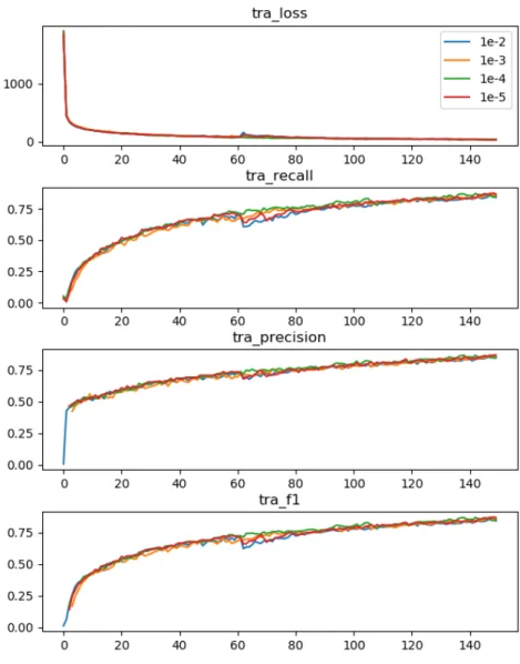
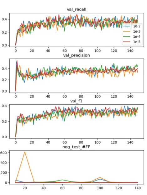
From the last experiment, it was discovered that the network overfits quite rapidly, there-fore several experiments were conducted by changing the value of the learning rate to check if the network can achieve better validation metrics before overfitting. Since the program uses the Adam[21] algorithm to alter the weight’s values, what is usually called learning rate in other optimisation algorithms in this case is called alpha (or effective step size), but it represents mostily the same concept as explained in the previous paragraph. Using Adam means that the learning rate will not be constant in every weight along the whole training process, instead it starts at a fixed value (alpha) and then it changes and adapts to the gradient of that specific weight, achieving better performance than other stochastic gradient descent optimisation algorithms. In the context of these experiments, the default value for alpha is 10−3, as suggested by the paper[21], but in order to find if this value is the best fit for the problem at hand, experiments were run with higher and lower powers of 10. The results of the experiments can be observed in the following graphs (Figure3.9, page34and Figure3.10, page35).

(40)

This may be caused by the pretrained weights. The model is initialised with values of a trained network which may cause the gradients to be small from the beginning, this is not expected to happen with models that start from a blank slate. If the amount of variation that needs to be introduced in each step is smaller than the smallest learning rate, all experiments would yield the same results.

Since it was discovered that altering the learning rate does not matter, the default value recommended by the Adam algorithm[21] of10−3will be used.

3.3.7 Object detection factors

The loss formula that is used by the network [13] is comprised of several factors, two of which weight the importance of detecting every object (even though it might be classified as a different class) and not making a detection where there is not an object. From now on these factors will be called object loss and non-object loss. Both of them have associated a fixed constant in order to balance the priority between finding all the target objects and not associating an object detection to the background of the image. These constant values will be called object scale and non-object scale respectively.

Since typically there is a lot more background area that there is object area in an image, it is clear that non-object loss will be a lower value most of the time, because a greater part of the detected background will coincide with the expected background. By default, object scale and non-object scale are weighted 1 to 100 in order to make non-object scale have a bigger impact in the total loss value. A reduction on this proportion would mean that the model would prioritise finding all the objects, taking less care in marking parts of the background as objects.

(41)

As it was expected, lowering the non-object scale decreases the penalty for getting false detections, the false positive rate increases and thus the precision is usually lower. This be-haviour happens because, if the model returns a big number of random detections, just by chance some of them will overlap with the targets and be considered as true positives thus achieving the higher values of recall as observed in the 1-25 ratio experiment. Not penalising all those extra detections would lead to a lower precision. Nonetheless, in the context of the dataset being studied, inferior values of precision do not necessarily mean bad performance, since, as it was said before, not all haemorrhages are annotated. In fact, in figure3.13(page38), it can be observed that a good number of false negatives do correlate to haemorrhage spots that are not annotated in the dataset. This concrete example only counts with a few ”true” false positives, for example the one in the lower left part of picture that just captures the top side of a healthy blood vessel and a flat background.

The difference is more clearly observed in the training metrics, where the different ratios are ordered in the recall metric, and reverse ordered in the precision metric. Nonetheless, in validation the difference is a lot more blurry. It is obvious that this parameter does not take a part in the number of false positives in negative images (just an anomaly is observed in 1-25 ratio epoch 30). But the decrease in precision observed in training is not clearly visible in validation. Looking at the validation metrics, it was decided that the 1-25 ratio is the most appropriate, as it achieves the highest recall and F1 score in validation but it does not see a high decrease in precision. Note that the 1-1 ratio was tested, but the network returned such a high amount of predictions that training was taking too long and the experiment was aborted.

To conclude, it was decided to keep the object and non-object scale correlation at a 1-25 ratio as a way of boosting the recall of the final system without hurting the precision and processing time too much.

3.3.8 Data augmentation

Data augmentation is the process of randomly changing the images in the dataset, increasing the number of training samples in order to improve the generalisation of the network. This process is specially useful when the amount of available data is limited, as in the HET-CAM problem. Some techniques involve mirroring the image in the horizontal or vertical axis (or both), scaling, rotating, or changing the colour of an image. In the context of this problem, due to the limited amount of training data, overfitting occurs quite rapidly so different aug-mentation methods were tested in order for the network not to learn the specific images of the training set.

(42)

size starts at its default value of416pxand is changed every 10 batches in random multiples

of32pxup to ±96px. These32pxintervals were chosen because they are compatible with

the internal structure of the network, specifically the downsampling or pooling layers, where the input is reduced to a fraction of its size. If the new size after downsampling or pooling is not an integer the model can have troubles or even crash. Apart from that, each image in a batch has a 50% chance of being flipped horizontally.

The video acquisition processes and the nature of the captured data cause luminosity and contrast heterogeneity within the HET-CAM frames. In order to have a more extensive rep-resentation of the data variability, changes in the colour of the image were also considered. In order to separate the raw colour from the lighting component, the images were converted to the HSV colour space, where they are split in the components of Hue (colour), Satura-tion (intensity) and Value (lighting). A script was developed to study the predominant H, S and V values in different images. The program orders the H, S and V values by number of appearances in each picture and then truncates that list to get the top values that account for>= 50% of the image. It was concluded that the predominant set of values across all of the videos of the dataset is composed of: Hue values ranging from 8º..24º, Saturation from 0.768..0.941, and Value from 0.549..1. The result of applying a random colour transformation with this values to a frame can be seen in figure3.14(page38)

Therefore in order to alter the pictures in a way that is not incoherent with the values observed in the dataset, fixed amount of variation in the HSV values was introduced. A ran-dom variation of±8H,±0.1S, and±0.1V was applied to the images with a 50% chance of happening. Having these random HSV transformation can help to artificially produce images that represent different lighting conditions, different egg colours, etc. The final state of the data augmentation pattern is the following:

• Every 10 batches the size of the image is changed from its initial size to up to±96pxin

intervals of32px

• A quarter of the time the image is left as is

• A quarter of the time the image is flipped horizontally

• A quarter of the time the image is changed colour in the HSV space: ±8H,±0.1S,

±0.1V

• A quarter of the time the image is both flipped and changed colour

(43)

Not only that, but, as it can be observed in figure 3.16(page 40), a very slight decrease in performance is caused by the use of data augmentation. Thus it can be concluded that data augmentation does not take a part on the performance of the network under the current cir-cumstances. It is conjectured that data augmentation does not make a big difference due to the very limited size of the dataset, since there are just 10 validation images. It is expected that with bigger datasets, data augmentation will help the model abstract the characteristics of the images and therefore have better performance. Nonetheless, data augmentation is usu-ally recommended [13] and therefore, as it does not help nor harm the performance of the model, it will be used in the final configuration.

3.3.9 Final network configuration

Throughout this section the impact of changing several parameters in the configuration of the network was studied. To conclude, a summary of the chosen configuration and the decisions made is presented.

First of all, the chosen implementation [19] advised to use pretrained weights for the convolutional layers of the network. Since the algorithm is commonly used for general object detection, specifically having different classes of objects to be recognised, it was considered that loading the pretrained weights might not play an important part in the context at hand, where only one type of class is present (a haemorrhage spot). From the experimentation carried out, it was concluded that loading the pretrained weights is advantageous, even if the dataset used has only one class and is very different to the ImageNet dataset.

From the pretraining experiment it was noted that the model overfits in a rapid manner and the validation metrics reach their maximum values in a low number of epochs. In order to give the model more time to evolve before overfitting, expecting an increase performance, lower learning rates were tested. It was found the default value of10−3is appropriate for the problem at hand, since, lowering it did not cause any change in performance.

Since the dataset is not exhaustively annotated, the measurement of false positives and precision rate needed to be carefully studied. It turned out that the network did detect some haemorrhages not tagged in the dataset and thus categorised them as false positives. The importance of finding all the annotated objects with respect to not finding too many false positives is balanced via the object and non-object scale factors in the loss formula. Exper-imentation was carried out varying these values in order to get the recall-precision balance appropriate for the context of this problem. The results pointed to a 1-25 ratio between object and non-object scale, to prioritise recall but still do not get a very low precision and number of ”true” false positives.

(44)

videos were transformed to the HSV colour space and their colour palettes were studied in order to set the bounds for random variations to be applied to the images in the dataset. Apart from that, several geometric transformations such as scaling and mirroring were applied to the images. The results were uncertain, data augmentation did not play a role, neither positive nor negative, in the performance of the network. This may be caused by the limited size of the dataset, so the final model configuration counts with data augmentation expecting that it will grant a positive outcome if the size of the dataset increases.

As a final note, the model does not achieve the standard values of recall, precision or f1 score that are expected for a state-of-the-art artificial intelligence system. It is, however, capable of distinguishing between positive and negative videos, as it can be seen from the number of false positives in negative test performance metrics. Taking into account that the validation metrics are calculated over several frames of different videos, but the program being developed studies the correlation between consecutive frames, the most important feature is that the model reacts similarly in similar frames in order to build a well formed graph of the evolution of the irritation process.

Therefore, with the final configuration of the network, the system’s performance needs to be checked by analysing its response to the test set. Since this set was not used to guide in any way the selection of the parameters, the metrics given by analysing it represent the real world performance of the system. Same as with the rest of the experiments, all the cross-validation folds were trained. Then, from each fold, the best epoch was chosen and passed through the test set in order to measure its performance.

As said before, a higher recall is a priority while choosing the best model in each fold. But, due to the high variability noticed in this metric along the experimentation, it is consider that basing this decision solely on the recall would be very volatile. So, in order retrieve a network with high recall but make sure that this value is not an anomaly, the sum of recall and f1 score was computed for each epoch and the highest value in each fold was selected. As the f1 score is biased by the precision, taking it into account ensures that the chosen model does not achieve a high recall value just by returning a big number of detections.

With the epochs selected for each fold, the metrics over the test set of that fold were computed. Table3.6(page30) shows the chosen epoch as well as its performance in the test videos, both positive and negative.

(45)

Fold Best Epoch Recall Prec. F1 neg. test FP

1 70 0.837 0.157 0.264 92

Table 3.6: Final configuration’s best epoch test metrics

4.5. In figure3.17(page41), which corresponds to the test performed by fold 1, this concept is clearly observed. It is clear that this kind of behaviour is of no use to the HET-CAM problem, but a positive note to take from this test is that it only happened in one of the folds, which means that it is not the working procedure of a standard trained network.

Considering the amount of haemorrhages tagged in the dataset and the metrics achieved,even taking into account fold 1, it is clear that the model will be capable of distinguishing very clearly between positive and negative videos. Take, for example, fold number 3 which only has 0.487 recall. That means that out of the 211 haemorrhages marked in video DSC_1098, the model correctly predicted around 102 of them, compared with just 9 false positives detected in the negative test. This means that even though the metrics values are low, in this context they are more than enough to determine if a video is positive or negative.

Not only that, but the model also returns a representative amount of the haemorrhages in each frame, which can be used to help in determining the toxicity of the drug. In this context, it is important that the system makes similar predictions in similar frames, as the HET-CAM study relates to the evolution of the irritation process, not the shear number of bleeding area. Therefore, low performance metrics do not imply that the model is unusable.

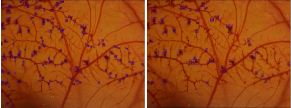
The following images correspond to the detections on the test set of fold 4, where the false negatives are highlighted in blue, false positives in red and true positives in green. In figure3.18(page41), it can be observed that the network does not detect all the haemorrhages targeted, but a good number of false positives do correspond to bleeding areas, double detec-tions our do not achieve the 0.5 IoU to be considered true positives. This kinds of values hurt a lot the numeric performance of the network, but upon visual inspection of the images, it can be seen that the amount of ”true” false positives does not correspond to a 0.45 precision. These images also show that the proportion between the confusion matrix values is mostly conserved as the video passes, therefore, from an bleeding evolution perspective, the model is expected to return a similar evolution curve when studying drugs that cause similar processes in the membrane.

(46)

true recall, precision and f1 scores better than the values displayed. Nontheless, this low theoretical values do not harm the performance of the network when analysing the evolution of bleeding areas.

3.4 Bleeding evolution module

The second module of the proposed methodology consists in gathering the information pro-vided by the bleeding detection module throughout all the frames composing the HET-CAM videos in order to extract objective information regarding the bleeding evolution. It was de-cided that the final program will be delivered as a Python scriptanalyse.py that allows the user to pick a video, analyses it using a trained model, and then shows number of detections and amount of bleeding area graphs in a Matplotlib[22] figure. By providing a script instead of an enclosed executable, the customisation of the program and output is maximised, allowing the users to change it to their needs. It is also recommended to have Pytorch installed with CUDA, as it hardware accelerates the analysis process and makes it a lot faster. This script does not count with a dedicated section in chapter4because it is a composition of parts of other scripts.

In order to feed the video frame by frame to the network, the (Pytorch) Dataset class was extended. The VideoDataset developed uses OpenCV[23] to read and return each individual frame. This can be easily changed to read a live video feed. Reading the whole video frame by frame can be slow, therefore, a parameter was introduced to ignore regular intervals of frames between samples.

The program first loads the trained model into memory and then opens the video selected by the user as a VideoDataset. It iterates over the dataset, analysing each individual frame and saving the number of detections and the area of bleeding. Since bounding boxes tend to overlap in areas with a high density of detections, the procedure used to calculate the total haemorrhage area is the union (instead of the sum) of all the areas detected. By doing this, counting twice the overlapping of areas is avoided, and a more reliable metric is calculated.

(47)

3.4. Bleeding evolution module

(48)

(49)

(50)

(51)

(52)

(53)

Figure 3.13: Example of model detecting more haemorrhages than the annotated by the dataset

(54)

(55)

(56)

Figure 3.17: Fold 1 test results of a frame: TP(green), FP(red), FN(blue)

(57)

(58)

Chapter 4

Software Development

For the accomplishment of the project’s objectives, several scripts and programs need to be developed. This chapter will detail the characteristics of each of them as well as the de-velopment process of the most complex ones from requirements, to design and finally their implementation.

The Python language was chosen for all of this operations because of the script-like nature of the problem. Its ease of use and the extensive amount of libraries like OpenCV [23] or Matplotlib [22], that make image processing and navigation easy and straightforward.

4.1 Image extraction and pre-processing

To perform the process of building an annotated dataset from the source videos, a number of steps need to be followed. First, the frames of interest need to be extracted from the videos and then each individual frame’s areas of bleeding need to be annotated following the specification described in section3.2.2.

(59)

4.1. Image extraction and pre-processing

Description A Python script that converts a video to a series of.png images, skipping a certain number of frames between samples

Input - Path to the video that wants to be converted - Number frames to be skipped

Output A folder with the extracted images in the same directory as the input video

Comments

Table 4.1: Specification ofFrameExtractor.py

Description A Python script that converts a set of 16:9 images into 4:3 aspect ratio. It saves the right and left sub-images for each input image

Input - Path to a folder of images that want to be converted

Output A folder within the selected folder containing the new 4:3 images

Comments

Table 4.2: Specification ofAspectRatioConverter.py

4.1.1 Design

First of all, the script that extracts frames from the videos,FrameExtractor.py, was designed. In order not to take too long, the amount of frames that are extracted per video is controlled by a parameter, allowing the user to skip a certain number of frames between saved images. The specification of the script is detailed in table4.1

At a later time, the need to change the image’s aspect ratio arose. It was decided not to redesign the previous script and re-process all the videos because the frames of interest were already filtered. Instead, a separate script,AspectRatioConverter.py, was designed to transform a set of 16:9 images into 4:3 aspect ratio. The images’ 4:3 resolution components will be calculated by keeping the current height constant and calculating the new width to get a 4:3 resolution. With that, two sub-images will be saved per input image, corresponding to taking the new width from the left and the right borders of the orinigal image. The specification of the script is detailed in table4.2

(60)

CHAPTER 4. SOFTWARE DEVELOPMENT

Figure 4.1: Aspect ratio converter: Input image - Left sub-image - Right sub-image

4.1.2 Implementation

The implementation of these two scripts was very similar, using TKinter to graphically ask the user for the parameters, be the video or the folder of images to be converted. Then, the whole behaviour of the script was encapsulated in a function with the specified inputs and outputs. The library chosen to open and save the videos and images was OpenCV[23]. Since both of the scripts are very simple and do not count with any custom class or other complicated structures, no use case, class or other kinds of diagrams were drawn.

(61)

4.2. Image marker

within the selected directory.

4.2 Image marker

The program described ahead was developed to act as a visual interface to help identify the bleeding areas and annotate them as described in section3.2.2. Its behaviour is best described by the use-case diagram depicted in figure4.2(page46)

Figure 4.2: Image Marker use case diagram

• Open image: The program opens a file system explorer window to help the user nav-igate to the image that needs to be annotated.

• Load marks: The system tries to open the text file that describes the areas marked in the picture; if it does not exist, the program continues.

• Visualise areas: The user is able to see all the objects marked in the current image.

• Change mode:The visualisation mode can change between showing the centre point of each area, or showing a rectangular outline of the bounding box.