Simulation of impulse response for indoor visible light communications using 3D CAD models

R E S E A R C H

Open Access

Simulation of impulse response for indoor visible

light communications using 3D CAD models

Silvestre Pérez Rodríguez

, Rafael Pérez Jiménez

, Beatriz Rodríguez Mendoza

,

Francisco José López Hernández

and Alejandro José Ayala Alfonso

Abstract

In this article, a tool for simulating the channel impulse response for indoor visible light communications using 3D computer-aided design (CAD) models is presented. The simulation tool is based on a previous Monte Carlo ray-tracing algorithm for indoor infrared channel estimation, but including wavelength response evaluation. The 3D scene, or the simulation environment, can be defined using any CAD software in which the user specifies, in addition to the setting geometry, the reflection characteristics of the surface materials as well as the structures of the emitters and receivers involved in the simulation. Also, in an effort to improve the computational efficiency, two optimizations are proposed. The first one consists of dividing the setting into cubic regions of equal size, which offers a calculation improvement of approximately 50% compared to not dividing the 3D scene into sub-regions. The second one involves the parallelization of the simulation algorithm, which provides a computational speed-up proportional to the number of processors used.

Keywords:Visible light communications, Ray-tracing, Impulse response, CAD models, Parallelization

1. Introduction

Recently, there has been a growing interest in visible light communications (VLC) in some indoor application sce-narios, video/audio transmission for in-home applications, secure network access, or sensor networking [1-8]. Fur-thermore, wireless optical communications present certain advantages over radiofrequency (RF) transmission that make them suitable in certain specific scenarios. Optical systems do not interfere with RF systems, thus avoiding electromagnetic compatibility restrictions. Moreover, there are no current legal restrictions involving bandwidth allo-cation and, since radiation is confined by walls, they pro-duce intrinsically cellular networks, which are more secure against deliberate attempts to gain unauthorized access than those relying on radio systems. In this sense, the characterization of indoor VLC channels, their time dispersion, and wavelength response is essential to study-ing and analyzstudy-ing the limits in terms of the design and performance offered by such links.

Simulating an indoor VLC channel can significantly benefit the design of high performance systems, but requires computationally efficient algorithms and models that accurately fit the characteristics of the channel ele-ments. In order to evaluate the impulse response for indoor VLC channels, two simulation algorithms can be adapted: the Barry and the López–Hernández algo-rithms. While the Barry algorithm is deterministic and based on an iterative method [9], the López–Hernández algorithm (called the Monte Carlo ray-tracing algorithm) is based on ray-tracing techniques and Monte Carlo method [10], which exhibits a lower computational cost than the Barry algorithm, especially when a high tem-poral resolution, complex geometries, and a large num-ber of reflections are considered. For this reason, in this article a tool for simulating the impulse response of in-door VLC channels using 3D computer-aided design (CAD) models is presented. The simulation tool is based on the Monte Carlo ray-tracing algorithm [10-12], and allows us to study the VLC signal propagation inside any simulation environment or 3D scene, regardless of its geometric shape, size (area), number of obstacles, etc. The tool features two fully differentiated parts. The first is charged with defining the 3D scene or the simulation

* Correspondence:[email protected] 1

Departamento de Física Fundamental y Experimental, Electrónica y Sistemas, Universidad de La Laguna, 38203, La Laguna, Tenerife, Spain Full list of author information is available at the end of the article

environment, which the user can describe by means of any CAD software that is capable of generating or stor-ing the scene in 3DS format. The geometry of the settstor-ing where the communications are being established, along with the different material types, emitters, and receivers that comprise the link or links involved in the simulation is specified in the 3D scene. The second element con-sists of implementing the propagation model. This refers to the mathematical models that characterize the effect of each of the elements present in the simulation envir-onment (reflecting surfaces, emitters, and receivers), and to the simulation algorithm that, aided by these models, allows the channel response to be computed. The part of the tool that implements the propagation model and into which the 3D scene is input is programmed in C++. In addition, so as to improve the computational effi-ciency of the simulation tool, two optimizations are pro-posed. The first one consists of dividing the simulation environment into sub-cubes of equal size, so that when a ray is traced in these sub-regions, only those object faces or surfaces that are in the ray propagation path need to be considered. This first optimization allows us to reduce the execution time by approximately 50% compared to not dividing the 3D scene into sub-regions. The second one consists of parallelizing the simulation al-gorithm. For each wavelength, the parallelization method proposed involves the equal and static distribution of the rays for computation by different processors, i.e., following a uniform distribution. This optimization results in a cal-culation speed-up that is essentially proportional to the number of processors used, i.e., when 2, 4, 8, and 16 pro-cessors are used, the computational speed-up increased by 2, 4, 8, and 16 times, respectively, with respect to using a single processor.

This article is organized as follows. In Section 2, the signal propagation model in an indoor VLC channel is defined; i.e., the Monte Carlo ray-tracing algorithm and mathematical models used to characterize the elements of the visible light link are described. Section 3 describes the main features of the simulation tool and its compu-tational complexity, which is compared with an alternate algorithm. The results are discussed in Section 4. Thus, several simulation results are reported to show the po-tential of the simulation tool and the effects on the com-putational speed-up due to both optimizations. Finally, Section 5 outlines the conclusions of this article.

2. Propagation model

As in conventional infrared wireless communication sys-tems, VLC uses intensity modulation and direct detec-tion for data transmission and detecdetec-tion. In general, for diffuse links, the indoor VLC system consists of an emit-ter, a receiver, and reflection surfaces. The propagation model is composed by the simulation algorithm and

mathematical models used to describe the features of the elements of the optical link. To evaluate the impulse response of the VLC channel, a Monte Carlo ray-tracing algorithm has been adapted [10-12]. In general, the multi-wavelength impulse response for an arbitrary pos-ition of emitterEand receiverRcan be expressed as an infinite sum of the form [9]

h tð;E;R;λÞ ¼hð Þ0ðt;E;R;λÞ

þX1

k¼1

hð Þk_{ðt;E;R;λÞ ð1Þ}

where h(0)(t;E,R,λ) represents the line-of-sight (LOS) im-pulse response,h(k)(t;E,R,λ)is the impulse response of the light undergoing k reflections, i.e., the multiple-bounce impulse responses,λis the wavelength, andtis the time.

2.1. LOS impulse response

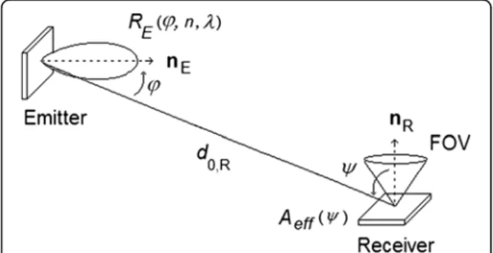
Given an emitter E and a receiver R in an environment free of reflectors (see Figure 1), with a large distanced0,R

between both [9], the LOS impulse response is approxi-mately

hð Þ0ðt;E;R;λÞ ¼ 1 d0;R

2REð’;n;λÞAeffð Þψ δ t d0;R

c

ð2Þ

where RE(’,n,λ) represents the generalized Lambertian

model used to approximate the radiation pattern of the emitter,cis the speed of light andAeff(ψ) is the effective signal-collection area of the receiver [9], which is given by

Aeffð Þ ¼ψ ARcosð Þψ rect ψ FOV

ð3Þ

where rect(x) is the rectangular function, whose value is 1 for |x|≤1 and 0 for |x| > 1,ARthe physical area of the

receiver, and FOV its field of view (semi-angle from the surface normal). In general, the emitter is modeled using a generalized Lambertian radiation pattern for each wavelength, and has axial symmetry (independent ofγ)

REð’;n;λÞ ¼nþ1

2π PEð Þλ cos n_{ð Þ’ ;}

π

2≤’≤π=2; 0≤γ≤2π ð4Þ =

where n is the mode number of the radiation lobe, which specifies the directionality of the emitter [9]. Integrating PE(λ) over the emitter wavelength

inter-val yields the nominal power PE emitted by the

emitter.

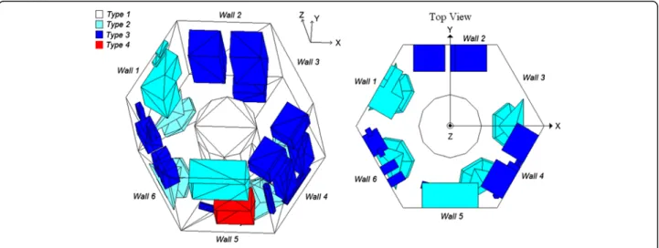
2.2. Multiple-bounce impulse responses

Consider an emitter and a receiver in an environ-ment with reflectors. Radiation from the emitter can reach the receiver after any number of reflections (see Figure 2). In order to calculate the multiple-bounce impulse responses using the Monte Carlo ray-tracing algorithm, many rays are generated at the emitter position with a probability distribution equal to its radiation pattern RE(’,n,λ). The power of each

ray generated is initially PE(λ)/N(λ), where N=N(λ)

is the number of rays used to discretize the source for each wavelength. When a ray impinges on a sur-face, the reflection point is converted into a new op-tical source, thus a new ray is generated with a probability distribution provided by the reflection pattern of that surface. The process continues throughout the maximum simulation time, tmax. After each reflection, the power of the ray is reduced by the reflection coefficient of the surface ρ(λ) and the reflected power reaching the receiver is computed.

For each wavelength, the power contribution of theith ray generated by emitter (1≤i≤N) after k reflections can be expressed by

Pi;kðE;R;λÞ ¼ 1

dk;R

2RS θk;R;θ

0_;λ

Aeff ψk;R

ti;k¼ Xk

j¼1 dj1;j

c !

þdk;R

c ð5Þ

whereti,krepresents the time instant in which the power

is detected by the receiver andRS(θk,R,θ’,λ) is the model

used to describe the reflection pattern. In this article, Phong’s model has been used [11,13]. In contrast to Lambert’s model, this model is able to approximate reflections consisting of both specular and diffusive components, which are described by

RS θk;R;θ0;λ

¼ρ_kð Þλ Pincð Þλ rd_πð Þλ cos θk;R

þ½1rdð Þλ mð Þ þλ 1

2π cos

m _θ

k;Rθ0

ð6Þ

The surfaces in Phong’s model are defined by three parameters for each wavelength: the reflection coeffi-cient ρk(λ), the percentage of incident signal that is

reflected diffuselyrd(λ), and the directivity of the

specu-lar component of the reflection m(λ). The parameters rd(λ) and m(λ) can be considered as independent for

each wavelength (unless in these simulations we con-sider them as constant). Furthermore,θk,Randθ’are the

observation angle and the incidence angle, respectively. Lastly, Pinc(λ) represents the optical power of the

incident ray before undergoing the kth reflection, which is given by

Pincð Þ ¼λ PEð Þλ N

Y k1 j¼1

ρ_jð Þλ ð7Þ

Summing the power contributions Pi,k in (5) for the

total numberNof rays, each undergoing a maximum of K reflections, and using the Dirac delta function to symbolize the time instants ti,k, yields the

multiple-bounce response, which is described by

X1

k¼1

hð Þkðt;E;R;λÞ¼X

N

i¼1

XK

k¼1

Pi;kðE;R;λÞ:δ tti;k

¼XN i¼1

XK

k¼1 1

dk;R

2RS θk;R;θ 0_;λ

Aeff ψ_k;R

:δ t X

k

j¼1

dj1;j

c

!

dk;R

c

!

ð8Þ

Substituting Equations (2) and (8) in (1), the total impulse response as a function of wavelength can be expressed as

h tð;E;R;λÞ¼ 1 d0;R

2REð’;n;λÞAeffð Þψ δ td0;R

c

þXN i¼1

XK

k¼1 1

dk;R

2RS θk;R;θ0;λ

Aeff ψk;R

:δ t X

k

j¼1

dj1;j

c

!

dk;R

c

!

ð9Þ

DefiningM=tmax/Δt, and assuming as the time origin the arrival of the LOS component, we can express the impulse response histogram as

h tð;E;R;λÞ ¼ 1 d0;R

2REð’;n;λÞAeffð Þψ δð Þt

þMX1

n¼1

XNn

i¼1

XKn

k¼1 1

dk;R

2RS θk;R;θ0;λ

Aeff ψk;R

:δðtnΔtÞ ð10Þ

where n symbolizes the nth interval time (width Δt) or bin of the power histogram. Furthermore,Knand Nnare

the number of reflections of theith ray and the number of rays that contribute in the nth time interval, respect-ively. This equation can also be written as

h tð;E;R;λÞ ¼ 1 d0;R

2REð’;n;λÞAeffð Þψ δð Þt

þMX1

n¼1

PnðE;R;λÞ:δðtnΔtÞ ð11Þ

wherePnrepresents the total received power in the nth

time interval.Pnis calculated as the sum of the power of

the Nn rays that contribute in that interval, which is

given by

PnðE;R;λÞ ¼X Nn

i¼1

Pi;nðE;R;λÞ

¼XNn

i¼1 XKn

k¼1 1

dk;R

2RS θk;R;θ

0_;λ

Aeff ψk;R

ð12Þ

wherePi,nis the total reflected power reaching the receiver

in thenth time interval due to theith ray propagation.

2.3. Error estimate of the simulated impulse responses

The use of an algorithm based on the Monte Carlo method allows for the error in computing the impulse response to be estimated with just one simulation run, as long as the number of rays is large enough. Although different error estimates are obtained for several simula-tions, we can be confident that the standard deviation of the estimates decreases as the number of rays is increased. Moreover, the method allows for the accuracy of the results to be assessed. The partial results of one simulation can also be used to achieve a more accurate solution by selecting a suitable number of rays.

In previous research [14,15], the equation that pro-vides an error determination when computing the im-pulse response was reported, which can be estimated as the square root of the total received power variance, var(Pn(λ)), in thenth time interval (widthΔt). Therefore,

for each wavelength the absolute error is given by

errðPnð Þλ Þ ¼pffiffiffiffiffiffiffiffiffiffiffiffiffiffiffiffiffiffiffiffiffiffivarðPnð Þλ Þ

¼

ffiffiffiffiffiffiffiffiffiffiffiffiffiffiffiffiffiffiffiffiffiffiffiffiffiffiffiffiffiffiffiffiffiffiffiffiffiffiffiffiffiffiffiffiffiffiffiffiffiffiffiffiffiffiffiffiffiffiffiffiffi XNn

i¼1

P2i;nð Þ λ 1 N

XNn

i¼1 Pi;nð Þλ

!2 v

u u

t _ð13Þ

where Pi,n is the reflected power reaching the receiver

(ith ray,nth time interval),Nnis the number of rays that

contribute in that interval,Nis the number of rays used to discretize the source, and Pn is the total received

power in the nth time interval, which was described in (12). Therefore, the relative error in a time interval Δt can be expressed as

rel errðPnð Þλ Þ ¼

ffiffiffiffiffiffiffiffiffiffiffiffiffiffiffiffiffiffiffiffiffiffiffiffiffiffiffiffiffiffiffiffiffiffiffiffiffiffiffiffi XNn

i¼1 P2i;nð Þλ

XNn

i¼1 Pi;nð Þλ

!2 1 N v u u u u u u u u t

ð14Þ

because we can estimate the number of rays needed to obtain results with the accuracy appropriate to the matter of interest. For example, if the relative error obtained is 4.5% for 100,000 rays, the number of rays needed to de-crease the error to 2% is 500,000 2_{ffiffiffiffiffiffiffiffiffiffiffiffiffiffiffiffi} ð %¼4:5%pffiffiffiffiffiffiffiffiffiffiffiffiffiffiffiffi100;000=

500;000

p

Þ. ConsideringΔTas the time elapsed between the initial time and every subsequent simulation instant, Equation (14) allows us to determine the cumulative error along the simulation time. Therefore, the relative cumula-tive error in a time intervalΔTcan be described by

rel cum errðPnð Þλ Þ ¼

ffiffiffiffiffiffiffiffiffiffiffiffiffiffiffiffiffiffiffiffiffiffiffiffiffiffiffiffiffiffiffiffiffiffiffiffiffiffiffiffiffi XNΔT

i¼1 Pi2;nð Þλ

XNΔT

i¼1 Pi;nð Þλ

!2 1 Nf v

u u u u u u u u t

ð15Þ

whereNΔTis the number of rays that contribute inΔTand

Nfis the number of flights of rays along that interval time.

3. Features of the simulation tool

In the following sections, the elements that constitute the simulation tool are described. Moreover, an equation that describes the computational complexity of the simulation algorithm based on the number of rays, num-ber of reflections, and geometric complexity of the simu-lation environment is presented.

3.1. Description of the simulation tool

The simulation tool developed allows us to estimate the impulse response of indoor VLC channels in time and wavelength using 3D CAD models. Figure 3 shows the block diagram of the simulation tool. The diagram reveals the two key elements that comprise the simula-tion software: the inputs of the simulasimula-tion tool that the user specifies by means of various files, and the propa-gation model described in Section 2, which consists of the simulation algorithm and the mathematical models

that characterize the effect of each element present in the optical link. In addition, the tool also includes a utility for displaying and analyzing the program’s exe-cution trace through a 3D viewer developed using Java 3D. The inputs of the simulation tool consist of the geometry of the simulation environment or 3D scene, the parameters of the reflection pattern of the materi-als comprising the reflective surfaces, the emitter and receiver locations, and other simulation parameters such as the number of rays, the maximum number of reflections, the maximum simulation time, emitter and receiver orientations, the emitter’s modal index, the receiver’s field of view, etc. While the user can describe the simulation environment geometry using any CAD soft-ware that is capable of generating or storing the 3D scene in a 3DS file, the remaining inputs are specified by means of auxiliary text files.

One of the main features of this tool is that it allows us to study the VLC signal propagation inside any simu-lation environment, regardless of its geometric shape, size (area), number of obstacles in its interior, etc. In general, any CAD software capable of generating 3D vector-type graphics and storing them in a 3DS-format file can be used. The 3DS file format, currently one of the most complete and widely used, contains informa-tion on meshes, material attributes, bitmap references, textures, display configurations, camera positions, lumi-nosity, and even data on object animations. The meshes comprise the elements or objects in the 3D scene, and consist of groups of triangles or faces. Each of these faces is defined by three vertices and has associated with it the properties of the material of which it is made, such as visibility, etc. These properties allow us to establish the reflective characteristics of the materials present in the simulation environment, that is, the way in which the incident rays are reflected. The simulation tool was developed in the C++ programming language and a lib3ds programming library was used to make it easier to work with the 3DS format.

3.2. Computational complexity

In contrast to other methods [8,9], the Monte Carlo ray-tracing algorithm allows for the evaluation of the impulse response for environments with complex geometries with no meaningful increase in computational cost, especially when a high temporal resolution, and a large number of reflections are considered. This can be explained by the number ofelementarycalculations that is performed:k N NF, whereNis the number of rays for each wavelength,k

is the number of reflections that are considered, andNFis

the number of faces or triangles that define the geometry. An elementary calculation is defined as the calculation of power contribution and delay from a point source (emitter or reflection point of a ray) to the receiver, as in (5), and the assessment of the propagation of the new generated ray to determine a new point source. This computational cost can be compared with other deterministic algorithms, such as Barry’s algorithm [9], where a total of (NC)k

elem-entary calculations is performed, andNCis the number of

elements into which the reflecting surfaces are divided. Therefore, the Monte Carlo ray-tracing algorithm requires a smaller amount of computational effort for a large num-ber of reflections (k) and a large number of triangles or faces (NF). We can also observe that the area of the

tri-angle is not important, in contrast to Barry’s algorithm, where the number of reflecting elements NC depends

upon the size of the surfaces. Moreover, Monte Carlo ray-tracing algorithms allow for the evaluation of the confi-dence levels of the simulation results. Despite being very accurate, deterministic methods do not allow for an easy evaluation of the error due to discretization. Also, they can compute the impulse response for just the lower-order reflections, allowing the simulation to be conducted in a reasonable amount of time since the run time is expo-nential in k. Thus, for example, to compute the k= 3 bounce impulse response with NC= 2,776 elements (an

empty rectangular room of 7.5 × 5.5 × 3.5 m3defined by six surfaces,NF= 12 triangles), the number of elementary

calculations is roughly 2.1 × 1010 (5.9 × 1013 for k= 4). The ray-tracing algorithm is able to obtain a simulated im-pulse response for the same room with a relative error of less than 1% usingN= 10,000,000 rays, which is equivalent to 3.6 × 108elementary calculations (4.8 × 108fork= 4). In short, fork =3 reflections, the Monte Carlo ray-tracing algorithm improves the computational efficiency 58-fold in comparison to using Barry’s algorithm. Fork= 4 reflec-tions, the improvement is 1.23 × 105fold.

4. Results

In this section, we present several simulation results to show the potentiality of the simulation tool to approxi-mately characterize the impulse response of indoor VLC channels. Moreover, the effects on the computational speed-up due to the two optimizations proposed for im-proving the computational efficiency are discussed.

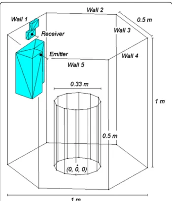
4.1. Application example

As an example of an application of the simulation tool developed, we studied the propagation of visible light in the simulation setting depicted in Figures 4 and 5. The 3D scene is a 1.0 × 1.0 m2hexagonal structure with dif-ferent objects or obstacles inside. The emitter and re-ceiver are located on wall 1 and oriented towards the interior of the 3D scene, i.e., there is no LOS communi-cation between emitter and receiver (see Figure 5). We should note that even though this example considers a single emitter and receiver, the tool can be used to simu-late the presence of multiple emitters and receivers in any 3D scene. To model the scene, we used the Blender graphic design program because it offers multi-platform support in a freeware product whose output 3DS file includes the simulation environment geometry, emitter

and receiver locations, as well as the characteristics of the different materials on the triangles that comprise the simulation environment. The 3DS-format file generated by the graphic design software constitutes one of the inputs to the simulation tool, which is capable of

interpreting the information stored in the graphic file to extract the location of the vertices and triangles used to model the 3D scene. In this case, the scene was modeled using 284 vertices and 416 triangles. Four types of mate-rials with different spectral reflectance characteristics were considered [16]. In addition to the information on the simulation environment provided by the graphic file, other parameters necessary to carry out the simulation must also be specified, such as the number of rays, the maximum number of reflections, the maximum simula-tion time, emitter and receiver orientasimula-tions, the emitter’s modal index, the receiver’s field of view, etc. All of these input parameters are extracted from auxiliary text files. The parameters stored in these files and used in the simulation are shown in Table 1.

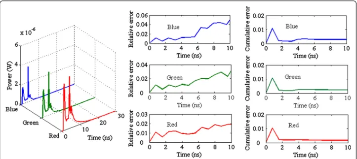
In terms of the simulation run time, we note that for a dual-core Intel Xeon 3.20 GHz processor with 1 GB of RAM running Debian GNU/Linux, the execution time was approximately 21 min (1,260 s). Figure 6 illustrates the impulse responses for RGB wavelengths, i.e., λRed= 635 nm, λGreen=525 nm, and λBlue=455 nm. The esti-mates of the relative and relative cumulative errors in computing the impulse responses are also given. We can see that the impulse responses show a similar temporal evolution for each wavelength, though with different power levels. This is because we assumed that only the reflection coefficient of the simulated materials depends on the wavelength, while the remaining parameters are constant (see Table 1). The error curves also present a similar shape. The small differences are due to the ran-dom nature of the simulation algorithm. We can see that the relative errors obtained are less than 5%, though in order to ascertain the accuracy of the impulse responses, the relative cumulative error must be examined. The maximum value for the relative cumulative error is given by blue wavelength, which is less than 0.3%.

As regards the computational complexity, since the number of rays considered in the simulation was N= 500,000, the number of triangles that define the 3D scene wasNF= 416, and the number of reflections wask

= 10, the number of elementary calculations per wave-length is 2.08 × 109. This computational cost can be compared to using Barry’s algorithm. If the total area of the reflecting surfaces (7.78 m2) is divided intoNC= 778

elements, i.e., an element area of 100 cm2 is used, the number of elementary calculations is 8.1 × 1028. Further-more, as discussed in Section 3.2, in the Monte Carlo ray-tracing algorithm the size of the reflecting surfaces is not important, in contrast to Barry’s algorithm, where the number of reflecting elementsNCincreases with the

size of the surfaces, or total area. Thus, for example, if the area is 70 m2(a hexagonal structure of 3.0 × 3.0 m2), i.e., NC= 7,000 elements, the number of operations

increases to 2.8 × 1038.

Figure 5Emitter and receiver locations and 3D scene dimensions.

Table 1 Simulation parameters

Parameter Value

Emitter Mode (n) 1

PE(λ), W 1/3

Position (x, y, z), m (₋0.25, 0.14, 0.83)

Orientation 90°, 330°

Receiver Active area (AR), cm2 1

Position (x, y, z), m (−0.33, 0.24, 0.91)

Orientation 90°, 330°

FOV 85°

Resolution Δt, ns 0.2

Bounces k 10

Number of rays N(λ) 500,000

Materials (Type) ρBlueρGreenρRed rd(∀λ) m (∀λ)

Wood (1) 0.25 0.43 0.73 1 –

White marble (2) 0.70 0.77 0.82 0.5 230

Aluminium metal (3) 0.45 0.49 0.52 0.3 250

4.2. Computational speed-up

In order to improve the computational efficiency of the simulation algorithm, we introduced two optimizations. The first one consists of dividing the 3D simulation en-vironment into a set of cubic sub-regions of equal size. The number of divisions to be made at each edgeccan be specified in the tool, thus generating a total of c3 grids. When tracing a ray, these grids allow for only those object faces and/or surfaces that are in the propagation path of the ray to be considered. This technique is equiva-lent to simplifying the ray propagation by considering only those surfaces that are actually involved in the propagation process, and is used for ray-tracing urban field prediction models [17]. With this optimization, the computation time is reduced without affecting the accuracy of the results. The second optimization is the parallelization of the Monte Carlo method. The Monte Carlo method is a nu-merical statistical method based on the generation of a set of random numbers to compute a set of results associated with each. The final solution is obtained by combining each sub-result. The parallelization of the Monte Carlo method usually involves distributing the computation associated with each random number to the various pro-cessors used in the execution. One possibility is to distrib-ute each computation statically, that is, dividing the computation equally among all the processors. If the com-putational effort associated with each random number varies too much, a static distribution could result in some processors completing their work well before others do. In these cases, methods for balancing the workload are used in an effort to make better use of the resources available. Since workload balancing methods introduce a certain

additional load on the processors, these methods should not be used when a static workload distribution will yield a good use of resources. In the case at hand, it is reason-able to assume that a static distribution will yield a better result than a balanced distribution due to the negligible variability in the computational cost associated with each ray; that is, it is unlikely that any one processor will have to compute a large amount of high-cost rays while others compute low-cost rays. Although each ray undergoes a different number of reflections, when the number of rays is large, the average number of reflections experienced by rays assigned to each processor is very similar. Thus, for example, for the simulation environment shown in Figure 4 with 500,000 rays, unlimited reflections, assuming that the minimum power detected by the photodetector is

Figure 6Simulated impulse responses and relative errors obtained for RGB wavelengths (λRed= 635 nm,λGreen= 525 nm, andλBlue= 455 nm).

10–12W, and statically distributing the rays among 16 pro-cessors, the average number of reflections per processor is 15.01 ± 0.02. When a smaller number of processors is used, the number of rays assigned to each processor is greater, resulting in a variation in the average number of reflections per processor of less than 0.02 (0.001 for two processors). That is why we propose the utilization of the static ray distribution parallelization method, where the rays are assigned to each processor with equal probability, i.e., fol-lowing a uniform distribution. Specifically, for each emitter involved in the simulation, each processor will be tasked with simulating a subset of rays for each wavelength.

In order to evaluate the effect of both optimizations on the computational speed-up, several simulations were performed using the same simulation environment and parameters as in the previous section (see Figure 4 and Table 1), though 24 simulated receivers were used, located in different positions within the 3D scene. For this case, without applying the optimizations, the simu-lation run time was approximately 472 min (28,332 s). Figure 7 shows the resulting sequential computing time as a function of the number of divisions, which allow us to determine the computational speed-up due to the optimization involving the use of sub-regions. The experi-ments were conducted on a Debian GNU/Linux cluster with eight dual-core Intel Zeon 3.20 GHz processors with 1 GB of RAM linked via a Gigabit Ethernet connection. The results clearly show that the use of grids decreases the computation time, though if the number of divisions is increased too much, the simulation performance suffers. This is due primarily to the fact that the initialization time and the memory requirements increase considerably with the number of divisions. Specifically, this optimization pro-vides a 50.6% improvement when the number of divisions is 70, which is the number that exhibits the best results in terms of the execution time. Figure 8 shows the computa-tional speed-up obtained from the second optimization proposed, which was to parallelize the algorithm for 2, 4, 8,

and 16 processors. As we can see, the behavior shown by the computational speed-up is practically proportional to the number of processors used, thus verifying the initial as-sumption that a static distribution is sufficient to ensure the proper use of the available resources.

5. Conclusions

In this article, we presented the design and implementa-tion of a simulaimplementa-tion tool to estimate the impulse re-sponse of indoor VLC channels in time and wavelength using 3D CAD models. The indoor VLC channel simula-tion can significantly benefit the design of high perform-ance VLC systems, but requires computationally efficient algorithms and models that accurately respond to the characteristics of the channel elements. In this sense, the simulation tool allows us to accurately define the simula-tion environment with 3D CAD models; furthermore, it is based on the Monte Carlo ray-tracing algorithm, which exhibits a lower computational cost than other algorithms, especially when a high temporal resolution, complex geometries, and a large number of reflections are considered. Therefore, one of the main features of the tool is that, for a given number of reflections and temporal resolution, it allows us to study the VLC signal propagation inside any simulation environment, regard-less of its geometric shape, size (area), number of obsta-cles in its interior, etc., with a high computational efficiency. Finally, in order to improve its computational efficiency, two optimizations were introduced. The first consisted of dividing the simulation environment into sub-cubes of equal size so that when a ray is traced in these sub-regions, only those object faces or surfaces that are in the ray propagation path need to be consid-ered. Defining the optimum number of divisions as the maximum possible value that does not saturate the node in terms of the amount of memory required, this first optimization yielded a 50.6% decrease in execution time compared to not dividing the 3D scene into sub-regions. The second optimization consisted of parallelizing the simulation algorithm based on an equal and static distri-bution of the rays generated at the emitter among the available processors, i.e., assigning the rays to each proces-sor by means of a uniform distribution. This optimization resulted in a computational speed-up that is essentially proportional to the number of processors used. In short, when 2, 4, 8, and 16 processors are used, the speed-up fac-tor increased by 2, 4, 8, and 16 times, respectively, with respect to using a single processor.

Competing interests

The authors declare that they have no competing interests.

Acknowledgments

This study was funded in part by the Spanish Ministerio de Ciencia e Innovación (project TEC2009-14059-C03-02/01/03), Plan E (Spanish Economy and Figure 8Speed-up factor as function of the number of

Employment Stimulation Plan), and the Government of the Canary Islands (project SolSubC200801000306).

Author details

1_{Departamento de Física Fundamental y Experimental, Electrónica y} Sistemas, Universidad de La Laguna, 38203, La Laguna, Tenerife, Spain. 2_{Instituto para el Desarrollo Tecnológico y la Innovación en Comunicaciones} - IDeTIC, Universidad de Las Palmas de Gran Canaria, 35017, Las Palmas de Gran Canaria, Spain.3_{Centro de Domótica Integral - CeDint, Universidad} Politécnica de Madrid, 28223, Madrid, Spain.

Received: 31 March 2012 Accepted: 27 November 2012 Published: 12 January 2013

References

1. KD Langer, J Vucic, C Kottke, LF del Rosal, S Nerreter, J Walewski, Advances and prospects in high-speed information broadcast using phosphorescent white-light LEDs, inProceeding of 11th International Conference on Transparent Optical Networks (ICTON’09), Azores, Portugal, 28 June–2 July, 2009, pp. 1–6

2. KD Langer, J Grubor, Recent developments in optical wireless communications using infrared and visible light, inProceeding of 9th International Conference on Transparent Optical Networks (ICTON_’07), Rome, Italy, 1–5 July 2007, vol. 3, pp. 146–151

3. T Komine, M Nakagawa, Fundamental analysis for visible-light communication system using LED lights. IEEE Trans. Consum. Electron.

50(1), 100–107 (2004). doi:10.1109/TCE.2004.1277847

4. H Lee, Y Kim, K Sohn, Optical wireless sensor networks based on VLC with PLC-Ethernet interface. WASET81, 245_–248 (2011)

5. PA Haigh, H Le Minh, Z Ghassemlooy, Transmitter distribution for MIMO visible light communication systems, inProceeding of 12th Annual Post Graduate Symposium on the Convergence of Telecommunications, Networking and Broadcasting (PGNet2011), Liverpool, United Kingdom, 27–28 June 2011,

pp. 190–193

6. PA Haigh, TT Son, E Bentley, Z Ghassemlooy, H Le Minh, L Chao, Development of a visible light communications system for optical wireless local area networks, inProceeding of Computing, Communications and Applications Conference (ComComAp), Hong Kong, China, 11–13 June 2012,

pp. 351–355

7. E Cho, JH Choi, C Park, M Kang, S Shin, Z Ghassemlooy, CG Lee, NRZ-OOK signalling with LED dimming for visible light communication link, in

Proceeding of 16th European Conference on Networks and Optical Communications (NOC), Newcastle-Upon-Tyne, United Kingdom, 20_–22 July 2011, pp. 32–35

8. K Lee, H Park, JR Barry, Indoor channel characteristics for visible light communications. IEEE Commun. Lett.15, 217_–219 (2011). doi:10.1109/ lcomm.2011.010411.101945

9. JR Barry, JM Kahn, EA Lee, DG Messerschmitt, Simulation of multipath impulse response for indoor wireless optical channels. IEEE J. Sel. Areas Commun.11(3), 367–379 (1993). doi:10.1109/49.219552

10. FJ López-Hernandez, R Pérez-Jiménez, A Santamaría, Ray-tracing algorithms for fast calculation of the channel impulse response on diffuse IR-wireless indoor channels. Opt. Eng.39(10), 2775–2780 (2000). doi:10.1117/1.1287397 11. S Rodríguez, R Pérez-Jiménez, FJ López-Hernádez, O González, A Ayala,

Reflection model for calculation of the impulse response on IR-wireless indoor channels using ray-tracing algorithm. Microw. Opt. Technol. Lett.

32(4), 296–300 (2002). doi:10.1002/mop.10159

12. S Rodríguez, R Pérez Jiménez, O González, J Rabadán, BR Mendoza, Concentrator and lens models for calculating the impulse response on IR-wireless indoor channels using a ray-tracing algorithm. Microw. Opt. Technol. Lett36(4), 262_–267 (2003). doi:10.1002/mop.10738

13. CR Lomba, RT Valadas, AM Oliveira Duarte, Experimental characterisation and modelling of the reflection of infrared signals on indoor surfaces. IEE Proc. Optoelectron.145(3), 191_–197 (1998). doi:10.1049/ip-opt:19982020 14. O González, C Militello, S Rodríguez, R Pérez-Jiménez, A Ayala, Error

estimation of the impulse response on diffuse wireless infrared indoor channels using a Monte Carlo ray-tracing algorithm. IEE Proc. Optoelectron.

149(5–6), 222–227 (2002). doi:10.1049/ip-opt:20020545

15. O González, S Rodríguez, R Pérez-Jiménez, BR Mendoza, A Ayala, Error analysis of the simulated impulse response on indoor wireless optical

channels using a Monte Carlo based ray-tracing algorithm. IEEE Trans. Commun.53, 124–130 (2005). doi:10.1109/tcomm.2004.840625

16. AM Baldridge, SJ Hook, CI Grove, G Rivera, The ASTER spectral library version 2.0. Remote Sens. Environ113, 711–715 (2009). doi:10.1016/j.rse.2008.11.007 17. V Degli-Esposti, F Fuschini, EM Vitucci, G Falciasecca, Speed-up techniques

for Ray tracing field prediction models. IEEE Trans. Antennas Propagat.

57(5), 1469–1480 (2009). doi:10.1109/TAP.2009.2016696

doi:10.1186/1687-1499-2013-7

Cite this article as:Rodríguezet al.:Simulation of impulse response for indoor visible light communications using 3D CAD models.EURASIP Journal on Wireless Communications and Networking20132013:7.

Submit your manuscript to a

journal and benefi t from:

7Convenient online submission 7Rigorous peer review

7Immediate publication on acceptance 7Open access: articles freely available online 7High visibility within the fi eld

7Retaining the copyright to your article