Characteristic time in quasispecies evolution

Characteristic time in quasispecies evolution

Arturo Marı´n

a

, He´ctor Tejero

a

, Juan Carlos Nun

˜ o

b

, Francisco Montero

a,n a

Department of Biochemistry and Molecular Biology I, Universidad Complutense de Madrid, Avd. Complutense s/n, 28040 Madrid, Spain b

Department of Mathematics Applied to Natural Resources, Escuela Te´cnica Superior de Ingenieros de Montes, Universidad Polite´cnica de Madrid, 28040 Madrid, Spain

a r t i c l e

i n f o

Article history: Received 27 July 2011 Received in revised form 20 January 2012

Accepted 29 February 2012 Available online 7 March 2012

Keywords:

Optimal mutation rate Evolution time Error threshold

Exploration–fixation trade-off

a b s t r a c t

The time a phenotype takes to achieve a stationary state from an initial condition depends on multiple factors. In particular, it is a function of both its fitness and its mutation rate. We evaluate the average time, referred to as the characteristic time,Tc, that the system takes to reach a final steady state of simple models of populations formed by self-replicative sequences. The dependence of Tcon the mutation rate and on the fitness landscape is also studied. For simple fitness landscapes, e.g. single peak, the characteristic time can be analytically obtained as a function of the system parameters. In this case,Tcfor obtaining the quasispecies distribution presents a maximum at aQ-value that depends on the initial conditions and decreases monotonously as the mutation rate tends to zero. For most of the complex landscapes handled in this paper, the characteristic time to achieve the quasispecies distribution picked around the fittest phenotype attains a local minimum for a given mutation rate between 0 and theQ-value at whichTcreaches its local maximum. Thus, in these cases, an optimum value for the mutation rate exists that corresponds to the lowest value of the characteristic time for quasispecies evolution.

&2012 Elsevier Ltd. All rights reserved.

1. Introduction

The quasispecies model developed byEigen (1971)is a useful general evolutionary model for error-prone self-replicative systems that has been applied in many different fields such as, for example, prebiotic self-replicating molecules (Schuster and Stadler, 2008), RNA viruses (Domingo et al., 2006), cancer cells (Sole´ and Deisboeck, 2004) and the immune system (Kamp et al., 2003). In all these problems, the question of how long the system takes to evolve is of great relevance. In particular, it is important to find out how this time depends on two of the main factors that govern evolution, namely the mutation rate and the fitness landscape.

In principle, as the mutation rate increases the time the system takes to evolve must decrease because the exploration through the sequences space is faster. However, the greater the value of the mutation rate, the higher the fraction of the less fitted mutant genotypes and, in consequence, the lower the average fitness of the population. In other words, the turnover of the whole population decreases, and therefore the evolution time increases. This trade-off between the generation of diversity and the fixation ability of advantageous mutants has been already described (Stich et al., 2007;Stich and Manrubia, 2011). For particular fitness landscapes, this balance is reflected in the appearance of a value for the

mutation rate at which the evolution time of the system presents a minimum. However, an explicit relationship between the opti-mum value of the mutation rate and the fundamental properties of the system, such as the characteristics of the fitness landscape, has not yet been exhaustively explored. Most of the models in which this problem has been examined are stochastic in nature. In this context different times have been defined, for instance, the searching time and fixation time (Traulsen et al., 2007; Gokhale et al., 2009; Stich et al., 2007; Stich and Manrubia, 2011), the evolution time (Krug and Karl, 2003) the adaptation time (Stich et al., 2007), the crossover time, the jump time, the residence time and the tunneling time (Jain and Krug, 2007;Krug, 2002).

Evolution is intrinsically a stochastic process. Phenotype existence depends on multiple factors that make it virtually impossible to be considered in its entirety. The birth and death of species occur according to probabilistic rules that, in the end, determine the population dynamics. Moreover, species interac-tion is also affected by randomness. Strictly speaking, mathema-tical models should include these stochastic factors to ensure a correct description of the population. However, it turns out that under particular conditions average variables can provide useful insights into the system’s behavior. In his seminal paper (Eigen, 1971) Manfred Eigen described the evolution of self-replicative molecules in terms of ordinary differential equations. Explicitly, he was assuming that stochastic fluctuations, whether internal or external, were, at a first approximation, not relevant and there-fore could be neglected. However, in the next section of his paper,

Contents lists available atSciVerse ScienceDirect

journal homepage:www.elsevier.com/locate/yjtbi

Journal of Theoretical Biology

0022-5193/$ - see front matter&2012 Elsevier Ltd. All rights reserved. doi:10.1016/j.jtbi.2012.02.029

n

he immediately went on to establish the limitation of this phenomenological description. In any case, the deterministic formulation brought about one of the most fruitful lines of research in evolution.

The deterministic modeling of populations formed by error-prone self-replicative sequences assumes that both the elementary process of mutation and the growth dynamics are free of stochas-ticity. Unfortunately, even under this approximation, finding the exact solutions for the phenotypes concentration is a very hard problem. Most of the mathematical analysis carried out on these dynamical systems is qualitative, i.e. it seeks to understand the asymptotic behavior of the system. It is implicitly assumed that (stable) equilibrium states are the unique observable outcome of actual systems. Nonetheless, this is not always true. During evolution we only observe transient regimes. The system is always evolving, although transient states can appear as metastables. In these models, time takes on a new meaning, not only as the continuous independent variable, but also as an observable of the system that deserves further attention. In particular, the time a dynamical system remains in a quasistationary state or the time taken to reach another quasistationary state are of special rele-vance. The problem arises when we want to characterize this time within a deterministic framework since, strictly speaking, this time is infinite because the trajectories approach the equilibrium points asymptotically. To measure this time, some authors have used the inverse of the largest eigenvalue or the inverse of the difference between the two largest eigenvalues, see for instance (Kamp et al., 2003; Nowak and Schuster, 1989). However, the application of these definitions even to simple continuous dynamical systems shows serious discrepancies.

The characteristic time, hereafter referred to as Tc (Llorens

et al., 1999), was previously defined to capture the global

evolutionary properties of dynamical systems. Based on a geome-trical interpretation, the characteristic time provides the average time the system takes to change from one state to another under the action of a perturbation or a persistent variation. For parti-cular linear dynamical systems, whose solution can be expressed as a linear combination of exponentials, the characteristic time corresponds to the average of the inverse of the exponents weighted by the pre-exponentials, real-valued constants that depend on the initial conditions and the matrix entries.

In general, the characteristic time depends on system para-meters in a more complex way. In the case studied here, it also depends on the mutation rate. To study this functional depen-dence this paper is organized from simple to complex models. Perhaps the simplest, though still interesting, system is the error-prone replication in a single peak fitness landscape, where a unique fittest phenotype and its indistinguishable mutants exist. Fortunately, as we will see inSection 2, this model allows a complete analytic treatment and thus, the obtention of an expression for the characteristic times for any initial condition as a function of the mutation rate and the amplification factors. For more complex landscapes, the characteristic times will be numerically computed for different parameter setups inSection 3. Finally, these results are discussed in the last section.

2. Characteristic time for a simple replicator system

We start by studying the characteristic time of a population formed by two self-replicative sequences. Fortunately, in this case the characteristic time can be analytically calculated, allowing a complete study of the dependencies with both the system para-meters and initial conditions.

Let us assume a dynamic system formed by two speciesI1and

I2, and letx1ðtÞandx2ðtÞbe their population at timet, respectively.

Without loss of generality we can assume a null death rate for both species. In the absence of any kind of constraint the time evolution of each of the population is given by the following system of ordinary differential equations (ODE):

_

x1¼Q1A1x1þ ð1Q2ÞA2x2

_

x2¼Q2A2x2þ ð1Q1ÞA1x1 ð1Þ

whereA1andA2are the amplification factors of speciesI1andI2,

respectively, and 0rQ1r1 and 0rQ2r1 are their respective

quality factors (i.e. 1Q1and 1Q2are the mutation rates forI1

andI2, respectively). Along this section, we will assumeA1ZA₂,

so I1 could be considered as the master copy, and I2 as the

error tail.

A complete description of the time evolution for each variable can be performed in terms of the molar fractions of each sequence. Let us define the molar fraction of the master sequence by

y1¼

x1

x1þx2

ð2Þ

Note thaty1A½0;1, and that the corresponding molar fraction of the sequenceI2is given byy2¼1y1. It is straightforward to find

the differential equation that describes the time evolution ofy1

from the previous Eq. (1)

_

y1¼ ð1Q2ÞA2þy1ðQ1A1A2ð1Q2ÞA2Þy12ðA1A2Þ ð3Þ

To complete the initial value problem we define the initial condition y1ðt¼0Þ ¼y01. Although non-linear, this equation is

still solvable, which will allow an analytical evaluation of the characteristic time according with the following definition. The characteristic time to achieve the equilibrium point from a given initial condition 0oy0

1o1 can be computed straightforwardly

using the equation

Tc¼

R1

0 t9y_19dt

R1

0 9y_19dt

ð4Þ

For a complete explanation of the meaning ofTcseeLlorens et al. (1999). According with this definition the characteristic time provides an average time to reach the equilibrium state from any initial condition along the trajectory. Let

gðtÞ ¼

9y_1ðtÞ9

R1

0 9y_1ðtÞ9dt

ð5Þ

be the density function obtained from the trajectory of variabley

fromy0at timet¼0 to the equilibrium point att¼ 1. Then, the

characteristic time is the first moment ofg, i.e.

Tc¼/tS¼

Z 1

0

tgðtÞdt ð6Þ

The initial value problem associated with Eq. (3) can be solved analytically. Ify1ðt¼0Þ ¼y0, the general solution reads

yðtÞ ¼ ypyn

y0yp

y0yn

eðynypÞt

1 y0yp y0yn

eðynypÞt

ð7Þ

where yp and yn are the equilibrium points of Eq. (3) (for simplicity the subindex 1 of the molar fraction is removed)

yp,n¼ 1 2

Q1A1ð1þ

E

ÞA27

ffiffiffiffiffiffiffiffiffiffiffiffiffiffiffiffiffiffiffiffiffiffiffiffiffiffiffiffiffiffiffiffiffiffiffiffiffiffiffiffiffiffiffiffiffiffiffiffiffiffiffiffiffiffiffiffiffiffiffiffiffiffiffiffiffiffiffiffiffiffiffi ðQ1A1ð1þ

E

ÞA2Þ2þ4

E

A2ðA1A2Þ

q

A1A2

ð8Þ

Here,

E

¼1Q2 is the mutation rate back from speciesI2to the

master copy, i.e. the probability of the production of master copies from its error tail. As it can be easily checked, only the equilibrium point with the positive root yp is non-negative (assuming A1A240) and then, has physical meaning. The

characteristic time can be analytically evaluated using Eq. (4) for the molar fraction of the master copy to reach the equilibrium pointyp

Tc¼ 1

A1A2

1

ypy0

ln ypyn

y0yn

ð9Þ

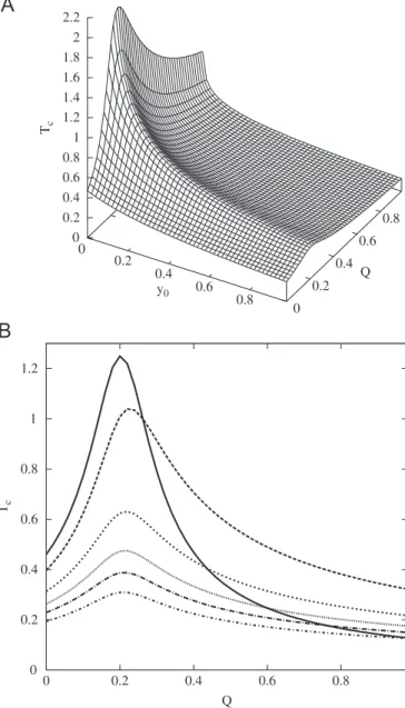
Fig. 1A shows the characteristic time as a function of the quality factor of the master copyQ1and the initial conditionsy0

when the back mutation rate is

E

¼102 _{and the amplification}

factors areA1¼10 and A2¼2. As it can be seen, Tc exhibits a

maximum for all values of the initial conditionsy0 at aQ-value

that will be referred as toQ1m(see alsoFig. 1B). The maximum value ofTc,Tmaxc andQ1mdepend on the initial conditions, as well as the rest of the parameters. Besides,Tmaxc depends on the value of

E

. In the limit of negligible back mutation rate, i.e. when

E

tends to 0, thenTmaxc tends to infinity atQ1m¼A2=A1, theQ-value that

corresponds with the error threshold.

It is worthy to compare the characteristic timeTcwith the time

scale given by the inverse of the eigenvalue of Eq. (3) (solid line in

Fig. 1B)

t

¼1

l

¼

1

ðA1A2ÞðypynÞ

ð10Þ

Obviously,

t

is independent of the initial conditions and attains its maximum at aQ-value, named asQ1c, that is given by

Q1c¼

A2

A1

ð1þ

E

Þ ð11Þ

Note thatQ1crQ1mfor all initial conditionsy0. As matter of

fact,Q1m-Q1c when y0-1. Moreover, contrary to what occurs

with the more complex landscapes we are going to investigate in the next sections, neitherTcnor

t

exhibit a minimum forQ-values larger thanQ1c(i.e. both are monotonous decreasing function of Q1in this range). The value ofTcatQ1¼1 is given by

TcðQ1¼1Þ ¼

1

A1A2

ln A1A2ð1

E

Þ

A1y0A2ðy0

E

Þ

1y0

ð12Þ

that tends to the same value as

t

wheny0-1 (seeFig. 1B)

TcðQ1¼1,y0¼1Þ ¼

t

ðQ1¼1Þ ¼

1

A1A2ð1

E

Þ

ð13Þ

The replicator model we have qualitatively analyzed in this section can be used to measure the characteristic time for several interesting processes that appear in quasispecies theory. In particular, (A) the selection of one of the species in a double peak landscape without mutation (whenQ1¼Q2¼1), (B) the dynamic

of two neutral species with different mutation rates (A1¼A2),

(C) the quasispecies formation from an error-prone replicator

without back mutations in a single peak landscape (whenQ2¼1

andQ14Q1c), and (D) the displacement of the master copy by the error tail beyond the error threshold (Q2¼1 andQ1oQ1c). The explicit expressions of the characteristic time for all these cases as well as for the general problem (E) are summarized inTable 1.

3. Characteristic time for the evolution in more complex fitness landscape

In the previous section we have treated a case that is analytically solvable, but real cases respond to more complex fitness landscapes, whose study requires numerical solutions. This section examines the characteristic timeðTcÞof a population of replicators that evolve in different fitness landscapes of increasing complexity.

0

0.2

0.4 0.6

0.8 y₀

0 0.2

0.4 0.6

0.8

Q 0

0.2 0.4 0.6 0.8 1 1.2 1.4 1.6 1.8 2 2.2

Tc

0 0.2 0.4 0.6 0.8 1 1.2

0 0.2 0.4 0.6 0.8

Tc

Q

3.1. A two peak separated by a neutral valley fitness landscape

Let us assume a mutation matrixQ¼ ½Qij that results from considering a classification of the sequence space according to the Hamming distance to the master copyI1. We consider a landscape

formed by two peaks separated by a degenerate valley. The two master copiesI1andI2are the two complementary bit string, i.e.

those formed by all 0 and all 1 digits, respectively. Their amplification factors areA1and A2, respectively. The rest of the

sequences have the same amplification factors,Ae. It is assumed thatA24A14Ae.

The probability that a sequence of the Hamming classl,Il, gives

rise to a sequence of the Hamming classk,Ik, is given byNowak and Schuster (1989)

Qk,l¼

X

minðk,lÞ

i¼lnþk

k i

n

k li

qn 1q q

kþl2i

ð14Þ

where

n

is the length of the sequences andqis the quality factor per digit. Since we are considering binary sequences, the total number of different sequences in the population is 2nand they are grouped into

n

þ1 Hamming classes.

The time evolution of the concentration of the Hamming class

Ij,xj, is described by

dxj

dt ¼AjQjjxjþ X

kaj

AkQjkxk ð15Þ

The corresponding differential equation for the molar fraction

yj¼

xj

P

ixi

is

dyj

dt ¼yj AjQjj

X

i

Aiyi

!

þX

kaj

AkQjkyk ð16Þ

If the quality factorqis large enough, this system has a unique steady state formed by a distribution of sequences that surrounds the fittest sequenceI2(Nowak and Schuster, 1989). Our intention

is to compute the characteristic time for the molar fraction of the copy I2 to achieve the steady state from an initial population

formed exclusively by copies of speciesI1. That is, we assume that

y1ðt¼0Þ ¼1.

The numerical integration of the ODE system was performed by a Runge–Kutta method provided by the MATLAB platform. The stop control was set to keep the difference between successive steps of variable I2 at less than 104 during 200 steps. The

characteristic time was then calculated, as described inLlorens

et al. (1999), by computing the quotient between the area,

computed by the classical trapezoid rule, over the trajectory of

I2 and below the horizontal asymptote that corresponds to its

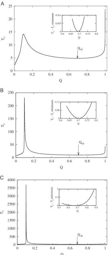
stationary value and the height of this asymptote.Fig. 2shows the dependence of theTcon theQvalue for different

n

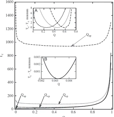
values (10, 20, and 50). This characteristic timeTcvaries with the quality factor per sequence Q¼qn _{in a different way as described in the} previous section. Whenqtends to 1, thenTcrises to infinity. In addition, Tc exhibits a unique maximum at a Q-value that, as before, will be referred to as Qm. Between these two values, Q¼QmandQ¼1, can be found a value ofQ, referred to as Qop, where the characteristic time reaches a local minimum (char-acterized by a null first derivative). The dependence of bothQop

andTcatQopon the valueA2andA1is shown inFig. 3for

n

¼10. In

all cases,A1¼4 andAe¼1, whereasA2takes the values: 10, 20, 40,

80, 100, 200, 300, and 400. As can be observed, asA2is increased

TcðQopÞdecreases. However, the functional dependence ofQopon

A2 is more complex, exhibiting a maximum value at an

inter-mediate value ofA2.

3.2. Multiplicative fitness with two peaks

Multiplicative fitness landscapes have been largely used in the framework of quasispecies theory (Woodcock and Higgs, 1996). In this section, we compute the characteristic time for the evolu-tion of the fittest sequence in the multiplicative fitness defined as follows. The amplification factor of each sequence at a Hamming distanceifrom the sequenceI0whose digits are all 0 is given by

Ai¼

ið1sÞðniÞ

n

!

9þ1 i¼1,. . .,

n

A0¼2 ð17Þ

where

n

is the chain length andsA½0;1allows to tune the effect that each mutation has on the fitness. In this way, the sequence whose digits are all 1, referred asIn, has an amplification factor

An¼10. Note that, for the special cases¼1, this fitness landscape Table 1

Characteristic timeðTcÞfor a quasispecies model of two replicators with different assumptions in relation with the value of both the mutation and the amplification factor matrix (A, B, C and D), as described in the text (Section 2). (A)Tcdepends not only on the difference between the amplification factors but also on the initial conditions. (B)Tccorresponds to the inverse of the eigenvalue of the linear Eq. (1). It is a decreasing function of bothQ1andQ2. (C)Tctends to infinity whenQ1tends toQcfrom above. It is a decreasing function ofQ1and tends to 1=ðA1A2ÞasQ1approaches 1. (D)Tctends to infinity whenQ1tends toQcfrom below. It is a increasing function ofQ1. (E)Tcreaches a finite maximum value atQ1mthat depends ony0. Besides, it is a decreasing function ofQ1forQ4Q1m.

Case Assumptions Initial value problem for molar fractiony Characteristic time (Tc)

(A) Q1¼Q2¼1

A14A2

_

y¼ ðA1A2Þyð1yÞ

yð0Þ ¼y0

Tc¼

1

A1A2ln

y0

y01

(B) A1¼A2¼A y_¼ ð1Q2Þ þyðQ1þQ22Þ yð0Þ ¼y0

Tc¼1

A 1 2Q1Q2

(C) Q2¼1

A14A2

Q14ðA2=A1Þ ¼Qc

_

y¼ ðA1A2Þy Q1A1

A2

A1A2

y

yð0Þ ¼1 Tc¼

ln Q1A1A2

A1A2

A1ðQ11Þ

(D) Q2¼1

A14A2

Q1oðA2=A1Þ ¼Qc

_

y¼ ðA1A2Þy

Q1A1A2

A1A2

y

yð0Þ ¼1

Tc¼

1

A1A2ln

Q1A1A2

A1ðQ11Þ

(E) A14A2 y_¼ ð1Q1ÞA2þyðQ1A1A2ð1Q2ÞA2Þy2ðA1A2Þ _T c¼ 1

A1A2

1

ypy0

ln ypyn

y0yn

reduces to the degenerate fitness landscape assumed in the previous section (where all the sequences between theI0 andIn are assigned the same amplification factor, 1). As the value of the parametersdecreases the change of the amplification factor tends to be linear with the Hamming distancei(Fig. 4, inset A).

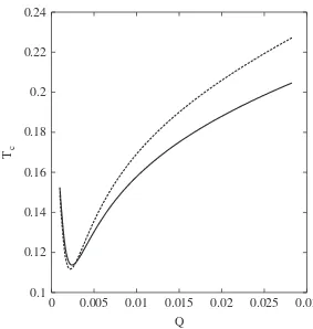
Fig. 4 shows the dependence of the Tc on Q for different

multiplicative fitness landscapes and

n

¼20. Using Eqs. (14) and (16), we determine the ODE systems that govern the time evolution of each species. These systems are numerically solved and then, the characteristic time Tc for In is estimated (all calculations are performed in MATLAB) (Fig. 4). As it can be seen, for the values ofslarger than 0.3,Tcexhibits two maxima, one for Q¼1 and the other for a low Q-value (approx. 0.1), and, as a consequence, a minimum atQop.

The insets B, C and D depict the classical figure of equilibrium population of the different Hamming classes (Schuster and Swetina, 1988) for the valuess¼0:3,0:6 and 1, respectively. Note that only for large values of s, e.g. s¼0.6 and s¼1, the steady populations change abruptly for aQ-value around 0.1, below which all sequences are equally populated. ThisQ-value corresponds to the error threshold,Qc. It is also worthy to remark that the value of

Qcestimated in these cases s¼0.6 ands¼1 approximately coin-cides with theQ-value for whichTcreaches its largest valueðQmÞ.

3.3. Binary rugged fitness landscape

Real fitness landscapes are rugged (Kauffman and Levin, 1987;

Kauffman and Johnsen, 1991;Schuster, 1997). In order to rise the ruggedness of the fitness landscape, let us now consider a population of binary sequences Ik,k¼1,. . .,2n whose fitness is related to the natural number codified in the sequence. Specifi-cally, let us assign to sequenceIkthe amplification factor

Ak¼

Nkþ1 2n

p

ð18Þ

Here,Nkrepresents the natural number codified byIkandpis an arbitrary positive natural number. This landscape is similar to that described in Nun˜ o et al. to study adaptive evolution of replicators (Nun˜ o et al., 2010). Note that with this definition 1=2nrAkr1 for allk¼1,. . .,2n. The largest amplification factor

A¼1 corresponds to the sequence whose digits are all 1. The parameterpdetermines the steepness of the landscape, i.e. as the

0

5

10

15

20

25

0

0.2

0.4

0.6

0.8

1

T

c

Q

0

50

100

150

200

250

0

0.2

0.4

0.6

0.8

1

T

c

Q

0

500

1000

1500

2000

2500

3000

3500

4000

0

0.2

0.4

0.6

0.8

1

T

c

Q

Qop

Qop

Qop

Fig. 2.Characteristic time ofI2in a double peak with a neutral valley as a function of the quality factors per sequenceQðQ¼qn_{Þfor several values of sequence} lengthsn: (A)n¼10, (B)n¼20, and (C)n¼50. In all cases,A1¼2,Ae¼1, and A2¼10. The insets clearly show the existence of the local minimum atQop.

0.65 0.66 0.67 0.68 0.69 0.7 0.71 0.72 0.73 0.74 0.75

50 100 150 200 250 300 350 4000

2 4 6 8 10

Qop

Tc

at Q

op

A₂

pvalue increases, the fitness landscape approaches a single peak landscape. In contrast to the fitness landscape studied in the previous section, different amplification factors now exist within the same Hamming class sequences. This fact prevents a simpli-fication of the mutation matrix similar to that used in Eq. (14). The probability of obtaining the sequence Ii during the error-prone self-replication of the sequenceIjis now calculated from the general formula

Qij¼ ð1qÞnqnn ð19Þ

wherenis the number of digits in which both sequences differ. This fitness landscape is rugged since sequences that differ in, for instance, only one digit can possess very different amplification factors, that is to say, they depend critically on the position of the digits.

The dynamics of the molar fraction of each sequence of the population is also governed by Eq. (16). The simulations were performed using the same algorithm in a MATLAB platform as described inSection 3.1. In all cases, a sequence length

n

¼10 was used. Thus, in this case, the dynamical system represented by Eq. (16) has 1024 ordinary differential equations and, each time, the variables satisfyPkykðtÞ ¼1. As in the previous section, initially all the population is formed by sequences of 0, i.e. y0¼1, and

whose amplification factor isA0¼ ð1=210Þp. The system (16) was

numerically solved for several values ofq, raging from 0.5 to 1, and for each value we computed the characteristic time asso-ciated with the molar fraction of the fittest sequence.

The results are shown in Fig. 5 for several values of the exponentp. As can be seen, the more relevant facts that appear in double peak landscape are reproduced. In particular, a value of

Qat which the value ofTcattains its minimum is observed. As the 0

50 100 150 200 250

0 0.1 0.2 0.3 0.4 0.5 0.6 0.7 0.8 0.9 1

Tc

Q

1 2 3 4 5 6 7 8 9 10

0 5 10 15 20

Amplification factor

Hamming Class

0 0.2 0.4 0.6 0.8 1

0 0.2 0.4 0.6 0.8 1

Steady concentration

Q

0 0.2 0.4 0.6 0.8 1

0 0.2 0.4 0.6 0.8 1

Steady concentration

Q

0 0.2 0.4 0.6 0.8 1

0 0.2 0.4 0.6 0.8 1

Steady concentration

Q

Fig. 4.Characteristic time of the fittest sequence in a multiplicative fitness landscape as a function of the quality factor per sequenceQfor different values ofs(from top to bottoms¼1,0:6,0:3,0:1 and 0, respectively). Inset (A) fitness landscapes for different values ofs(from top to bottoms¼0,0:1,0:3,0:6 and 1, respectively). In insets (B), (C) and (D) steady concentrations as a function ofQforsequal to 0.3, 0.6 and 1, respectively. In all casesn¼20.

0 200 400 600 800 1000 1200 1400 1600

0 0.2 0.4 0.6 0.8 1

Tc

Q

Q_op Q_op Q_op

Q_op

0 2 4 6 8

0 0.2 0.4 0.6 0.8 Tc

- T

c

minimum

Q

0 0.001 0.002 0.003

0.002 0.003 0.004 Tc

- T

c

minimum

Q

value ofpincreases, theTcvalue increases. This is a straightfor-ward consequence of the fact that the average productivity of the populations decreases withpat anyqvalue. Moreover, the

Qop-value also increases withp. This fact does not have an evident explanation since aspincreases the average productivity of the population decreases, while the apparent superiority of the fittest sequence increases. So, the compromise between the searching time and fixation time must vary.

3.4. NK fitness landscape

The NK model was introduced by Stuart Kauffman in the beginning of the nineties to study coevolution in simple organ-isms (Kauffman and Weinberger, 1989; Kauffman and Johnsen, 1991). Here,Ncorresponds to the chain length

n

, i.e. the number of positions of each sequence, whereasKð0oKoNÞ, represents the number of positions that influence on the contribution of a given position to the sequences fitness. This model generates fitness landscapes whose ruggedness increases withK.

In the classical version, theKpositions that are related to each position are randomly assigned. Therefore, each position can provide 2Kþ1

values of fitness, that are computed at random, depending on its actual state and the state of theKpositions that interact with it. The fitness of each species (sequence) is obtained from the average of the fitness of itsNdigits. As a consequence of these ‘‘long distance’’ interactions among the positions, sequences that belong to the same Hamming class could have very different fitness values, giving rise to rugged fitness landscapes.

Fig. 6depicts the dependence of the characteristic time Tcon the quality factorQ in two NKfitness landscapes forN¼10 and

K¼2 and K¼3. The population dynamics (as in the previous section, there are 1024 sequences) is again driven by Eq. (16), with the entries of the mutation matrix given by Eq. (19). As can be seen, in both cases the characteristic timeTcexhibits a local minimum at

Q-values close to the natural error threshold (located atQ¼1=2nÞ, respectively,Qop¼0:0024 forK¼2 andQop¼0:0022 forK¼3.

4. Discussion

In this paper, we have studied the dependence of the char-acteristic time on the mutation rate for different fitness

landscapes. It is expected that, as a consequence of the trade-off between the searching process inherent to any error-prone system and the rate of fixation of new fitter mutants a value of

Q at which the evolutionary time is minimum must exist. This opens interesting questions in evolutionary theory (Stich et al., 2007,2010a,b;Stich and Manrubia, 2011).

The problem of evaluating this time is enormous. On the one hand, controlling transient events in complex systems is extre-mely difficult. On the other hand, ensuring that the system achieves a new stationary state is also risky. The time scale in continuous dynamical systems has been defined as the inverse of the module of the largest eigenvalue or, in some cases, as the inverse of the module of the difference between the two largest eigenvalues (Nowak and Schuster, 1989). However, its validity must be reconsidered since these definitions provide bad estima-tions even in simple linear dynamical systems since they only yield information about the approximation to a final state from its vicinity, and they do not take into account the initial conditions of the system. The characteristic time, on the contrary, takes into account the complete trajectory of the system, from an initial condition to the final stationary state. Therefore, the character-istic time is an average time and so, like any other average, can hide information relevant to the study of the system, such as the variation of the higher order moments. We are currently inves-tigating the possibility of decomposing the characteristic time in different contributions (for example, searching time and fixation time) to avoid this limitation.

In Section 2, we have studied a population formed by two

replicators with non-null back mutation rate and an explicit solution for Tc has been obtained Eq. (9). This analysis has provided the functional dependence of the characteristic time on the mutation rate and amplification factors for different initial conditions. Tc depends inversely on the selection coefficient of species I1 over species I2, s¼A1A2, a result similar to that

obtained by Johnson (1999) using a completely different approach. Contrary to the time obtained from the inverse of the eigenvalue,Tcalso depends on the initial conditiony0. Naturally,

as the initial condition is closer to the equilibrium point, Tc

approaches the time provided by the inverse of the eigenvalue (Fig. 1B). WhenTcis plotted as a function of the quality factorQit exhibits a global maximum at aQ-value,Q1m, that depends ony0

and that tends to the error thresholdQcasy0tends to 1.

Unfortunately, analytical solutions can only be found for simple systems. Notwithstanding this, although analytical expres-sions cannot be obtained in more complex systems, a numerical approach can be used. The characteristic time can be numerically obtained as its computation only requires knowledge of the trajectory, without an explicit definition of the dynamical system. In other words, the characteristic time can be applied in a semiempirical approach to study evolutionary processes described by arbitrary complex models, if a numerical solution is provided. Using this approach we have studied the dynamics of adaptation in some more complex systems inSection 3.

It is well known that, independently of the fitness landscape, an equal distribution of the sequences of the population in the equilibrium of selection is obtained forQ¼1=2n. For some fitness landscapes this equidistribution of sequences occurs for a

Q41=2n. This Q-value is usually called error threshold and denoted as Qc. As can be deduced from the results obtained in this paper, in the situations when an error threshold exists, e.g. the single-peak landscape and the multiplicative landscape for high enough values ofs, the characteristic timeTcalways exhibits a local maximum at aQ-valueQmclose toQc. In those cases where there is not evidence of the existence of an error catastrophe,Tc

can present or not a largest value atQ¼1=2n. As a matter of fact, while in the multiplicative fitness studied inSection 3.2for low 0.1

0.12 0.14 0.16 0.18 0.2 0.22 0.24

0 0.005 0.01 0.015 0.02 0.025 0.03

Tc

Q

values ofs,Tcdoes not exhibit a maximum, this local maximum of

Tc appears in the rugged fitness landscapes used in Sections 3.3 and 3.4.

When a second maximum ofTcappears asQtends to 1, e.g. in fitness landscapes with more than one peak, a lowest value of the characteristic time is attained atQop, in betweenQmandQ¼1. This lowest value depends on the fitness landscape and, in particular, on the size of the sequence and on the superiority of the master phenotype over the rest of the phenotypes (seeFig. 3). In the NK fitness landscape this minimum occurs very near the natural limit

Q¼1=2nand then its relevance for evolution is questioned since the concentration of the fittest copy is very low. In the other cases, however, the minimum is achieved at larger values ofQ.

Note that, despite the flat appearance of the curve ofTcas a function ofQin the neighborhood ofQop(Fig. 2), small differences in the value of Tc could have strong consequences on the competitive dynamics of populations (as occurs with the tiny difference in the amplification factors). The question of how natural selection magnifies these small differences in finite size populations is currently under study.

Acknowledgments

This paper has been supported in part by Grants no. BFU2006-01951-BMC from MEC (Spain), by project FIS2009-13690 of the Ministerio de Ciencia e Innovacio´n de Espan˜ a and grant Q060120012 of the Universidad Polite´cnica de Madrid. Arturo Marı´n is supported by Consejerı´a de Educacio´n de la Comunidad de Madrid (Spain) and Fondo Social Europeo (FSE); and He´ctor Tejero is supported by AP2006-01044, from MEC (Spain).

References

Domingo, E., Martı´n, V., Perales, C., Grande-Perez, A., Garcı´a-Arriaza, J., Arias, A., 2006. Viruses as quasispecies: biological implications. Curr. Top. Microbiol. Immunol. 299, 51–82.

Eigen, M., 1971. Self-organization of matter and the evolution of biological macromolecules. Naturwissenschaften 58, 465–523.

Gokhale, C.S., Iwasa, Y., Nowak, M.A., Traulsen, A., 2009. The pace of evolution across fitness valleys. J. Theor. Biol. 259, 613–620.

Jain, K., Krug, J., 2007. Deterministic and stochastic regimes of asexual evolution on rugged fitness landscapes. Genetics 175, 1275–1288.

Johnson, T., 1999. The approach to mutation-selection balance in a infinite asexual population, and the evolution of mutation rates. Proc. R. Soc. Lond. B 266, 2389–2397.

Kamp, C., Wilke, C.O., Adami, C., Bornholdt, S., 2003. Viral evolution under the pressure of an adaptive immune system: optimal mutation rates for viral escape. Complexity 8 (2), 28–33.

Kauffman, S.A., Levin, S., 1987. Towards a general theory of adaptive walks on rugged landscapes. J. Theor. Biol. 128, 11–45.

Kauffman, S.A., Weinberger, E.D., 1989. The NK model of rugged fitness landscapes and its application to maturation of the immune response. J. Theor. Biol. 141, 211–245.

Kauffman, S.A., Johnsen, S., 1991. Coevolution to the edge of chaos: coupled fitness landscapes, poised states, and coevolutionary avalanches. J. Theor. Biol. 149, 467–505.

Krug, J., 2002. Tempo and mode in quasispecies evolution. In: L ¨assig, M., Valleriani, A. (Eds.), Biological Evolution and Statistical Physics. Springer, Berlin/Heidel-berg, pp. 205–216.

Krug, J., Karl, C., 2003. Punctuated evolution for the quasispecies model. Physica A 318, 37–143.

Llorens, M., Nun˜ o, J.C., Rodriguez, Y., Melendez-Hevia, E., Montero, F., 1999. Generalization of the theory of transition times in metabolic pathways: a geometrical approach. Biophys. J. 77, 23–36.

Nowak, M., Schuster, P., 1989. Error thresholds of replication in finite populations mutation frequencies and the onset of Muller’s ratchet. J. Theor. Biol. 137, 375–395.

Nun˜ o, J.C., de Vicente, J., Olarrea, J., Lo´pez, P., Lahoz-Beltra´, R., 2010. Evolutionary daisyworld models: a new approach to studying complex adaptive systems. Ecol. Inf. 5, 231–240.

Schuster, P., 1997. Landscapes and molecular evolution. Phys. D: Nonlinear Phenom. 107 (2–4), 351–365.

Schuster, P., Swetina, J., 1988. Stationary mutant distribution and evolutionary optimization. Bull. Math. Biol. 50 (6), 635–660.

Schuster, P., Stadler, P.F., 2008. Early replicons: origin and evolution. In: Domingo, E., Parrish, C., Holland, J.J. (Eds.), Origin and Evolution of Viruses. Elsevier, Oxford, pp. 1–42.

Sole´, R.V., Deisboeck, T.S., 2004. An error catastrophe in cancer? J. Theor. Biol. 228, 47–54.

Stich, M., Briones, C., Manrubia, S.C., 2007. Collective properties of evolving molecular quasispecies. BMC Evol. Biol. 7, 110.

Stich, M., Manrubia, S.C., 2011. Motif frequency and evolutionary search times in RNA populations. J. Theor. Biol. 280, 117–126.

Stich, M., Manrubia, S.C., La´zaro, E., 2010a. Variable mutation rates as an adaptive strategy in replicator populations. PLoS One 5, 6.

Stich, M., La´zaro, E., Manrubia, C.S., 2010b. Phenotypic effect of mutations in evolving populations of RNA molecules. BMC Evol. Biol. 10, 46.

Traulsen, A., Pacheco, J.M., Nowak, M.A., 2007. Pairwise comparison and selection temperature in evolutionary game dynamics. J. Theor. Biol. 246, 522–529. Woodcock, G., Higgs, P.G., 1996. Population evolution on a multiplicative