1. INTRODUCTION
As one of the main elements of geometric design, sight distance must be considered carefully for the safe and efficient operation of highways. In response to this, highway geometric design standards in dif-ferent countries set minimum sight distance thresh-old values (Ministerio de Fomento 2016, AASHTO 2011, FGSV 2012). In order to facilitate the geomet-ric design of roads, some guidelines propose two-dimensional analytical procedures to estimate the available sight distance. Nevertheless, these proce-dures may not be practical since they consider sepa-rately horizontal and vertical alignment, which may lead to overestimate or underestimate the actual available sight distance (Ismail & Sayed 2007). It is more common instead, to develop algorithms based on line-of-sight loops in three dimensions (3-D). Such procedures retrieve the cross-sectional profile of the terrain below the line of sight between the ob-server and the target locations, detecting whether the vision is obstructed. Ismail and Sayed (2007) de-vised a precise algorithm to compute the available sight distance. Besides algorithms based on line-of-sight loops, procedures based on viewsheds were
developed to study sight distance on highways (Cas-tro et al. 2011, Jha et al. 2011).
Computer-aided applications for road design es-timate and compare available sight distances to stopping sight distance and passing sight distance. They also include visualization tools that simulate the driver’s perspective while travelling (Kühn et al. 2011, Castro 2012). Such visualization tools are uti-lized to supervise proper 3-D alignment coordina-tion, although it requires this checking procedure is performed by experienced engineers (Larocca et al. 2011).
Methods based on line-of-sight loops enable the depiction of sight-distance graphs. These charts rep-resent on the horizontal axis the stations where the driver is sequentially placed, and on the vertical axis the sight distance variables ahead each driver posi-tion (Kühn & Jha 2011, Castro et al. 2014). Besides the comparison available and required sight distanc-es, such charts result advantageous to evaluate the 3-D alignment coordination (Roos & Zimmermann, 2004, Jha et al. 2011, Castro et al. 2015a). The Ger-man Road and Transportation Research Association provided a framework both for virtual perspective generation and sight-distance graphs on the design of
A comprehensive methodology for the analysis of highway sight
distance
M. Castro & C. De Santos-Berbel
Dep. Civil Engineering: Transport and Territory, Technical University of Madrid, Spain
L. Iglesias
Dep. Geological and Mining Engineering, Technical University of Madrid, Spain
rural highways (FGSV 2008). Campoy-Ungría (2015) proposed a procedure to estimate available sight distance on highways based on prismatic line-of-sight buffers launched directly on a high-density LiDAR cloud of points, not requiring any terrain sur-face.
A geographic information system (GIS) is useful to calculate sight distances because it gathers nu-merous advantages. Besides the 3-D treatment of the sight distance issue, it enables safety integrated anal-yses accounting for other factors such as geometrics, accident data, traffic volume, operating speed and design consistency at ease (Altamira et al. 2010; Castro & De Santos-Berbel 2015). Nowadays, af-fordable data sources are available to characterize the highway and the roadsides with higher accuracy, which GIS is capable of handling and exploiting at ease. Khattak and Shamayleh (2005) assessed high-way safety through GIS data visualization.
This paper reviews the GIS-based methodology developed to study sight distance on highways. The main issues are contemplated by means of case study examples. Following this introduction, the second section provides detailed description of the method-ology. Particular attention is paid to inputs (driver’s eye height, target height, vehicle path and elevation model) and output (sight distance graph). In the third part, case studies are presented. The first case illus-trates the influence of roadside elements (vegetation) through the use of a digital terrain model (DTM) and a digital surface model (DSM). The second one de-scribes how to detect and analyze shortcomings in the spatial alignment of highways through the use of sight-distance graph. The third one proposes a solu-tion based on GIS tools (lines of sight) and mul-tipatch datasets in order to represent overhanging roadside features (e.g. cantilever traffic signal) ade-quately. Finally, conclusions are presented.
2. METHODOLOGY
2.1 Sight distance algorithm
An application developed on ArcGIS was conceived for the 3-D estimation of available sight distance on highways and has already been validated by the au-thors (Castro et al. 2014). It is capable of computing the available sight distance of a highway section giv-en the driver’s eye height, the target height, the vehi-cle path and an elevation model.
The computational routine for available sight dis-tance estimation launches a line-of-sight beam itera-tively from every station on the vehicle path towards the stations ahead, determining whether each target is seen by the driver. Once the loop from a station has been completed, the virtual driver is moved for-ward to the next station, where an identical loop is launched. Available sight distance is defined as the distance, measured along the vehicle path, between
the driver’s position and the farthest target seen without interrupting the line of sight. According to this definition, the algorithm checks lines of sight from the driver position as shown in Figure 1. At station i, the available sight distance is determined by the station i+2 (line of sight in green), which is the furthest one seen before the first line of sight is blocked (station i+3, with line of sight in red). Soft-ware stores the binary value of visibility of every line of sight.
Figure 1. Available sight distance estimation through lines of sight.
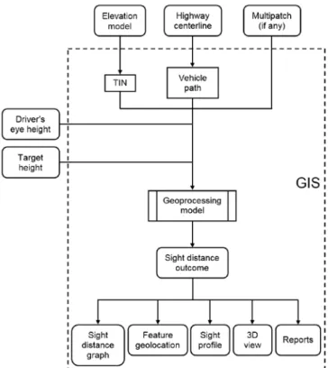
Figure 2 shows the complete process to study sight distance on highways, including the input and output data as well as the auxiliary tools developed.
Figure 2. Flowchart of the sight distance study procedure.
2.2 Input data
With respect to DEMs, the two types mentioned in the previous section are available for sight dis-tance modelling: DTM’s and DSM’s. Either of them is handled by the application as long as it is of the form of a triangular irregular network (TIN). To choose one over the other is not a trivial matter ow-ing to their influence in results. A DTM is a 3-D rep-resentation of the terrain surface which depicts ex-clusively the elevation of the bare ground. However, the reality contains many more elements influencing sight distance than the bare ground. Features such as vegetation, traffic signs, buildings and many other elements are not included in a DTM. These models comprise such additional roadside features, making available further information about features by the roadsides which could limit the available sight dis-tance. However, where overhanging features are pre-sent by the roadsides, the intrinsic features of DSMs hamper sight distance analysis. These surfaces do not support two points on its surface having the same horizontal projection while their elevation val-ues are different. This fact hinders a lifelike repre-sentation of overhanging features, which is particu-larly troublesome when they are partially located above the road, as occurs for tree crowns or cantile-ver signals.
Current techniques provide cost-effective high resolution DEMs. The remote sensing LiDAR (Light Detection And Ranging) devices emit a pulse beam. The pulse is received back if any surface is hit, which allows its geospatial location and its charac-terization (Topcon 2010). Usually, those data might have been collected by airborne surveying or terres-trial surveying. The latter ones are known as Mobile Mapping Systems (MMS). Whereas the airborne LiDAR is able to capture around one point per two m2, the MMS is able of deliver more than 200 points per m2 when closer to the sensor. However, the area covered from the airborne standpoint is much greater and the performance much higher, whilst the MMS are limited by elements that may create shadow areas beyond them. In both cases, raw data usually contain much noise. Items not forming part of the static landscape are captured, such as vehicles or even wildlife. Moreover, the abovementioned overhang-ing elements, i.e. aerial power lines, hamper the use of DSM. All those points are therefore entitled to be removed.
The shape of roadside elements is another fact to bear in mind. DSMs from airborne LiDAR can hardy model vertical roadside features, such as traffic signs or guard-rails, although they could represent consid-erably larger vertical devices (e.g. gantries) depend-ing on the resolution. In general, roadside vertical equipment is better depicted by DMSs derived from terrestrial LiDAR.
Regarding the trajectory, points that compose driver’s path could be obtained from several sources. If the highway geometrics are known, a theoretical
vehicle path can be extracted. Otherwise, it might be deduced from inventories or precise-enough carto-graphic data. Moreover, the track of a GNSS receiv-er mounted on a car driving along the studied high-way constitutes a reliable data source for this input when highway geometrics are unknown or not relia-ble. The application has tools that simplify its treat-ment. Points should have an attribute, namely sta-tion, which indicates their distance to the origin measured along this trajectory.
As generic inputs, driver’s eye height and target height must be considered. Those values are usually taken from highway design standards (AASHTO 2011, Ministerio de Fomento 2016).
The accuracy and resolution of these models, along with the spacing between the path stations, come also into play. The effect of these factors has been studied by the authors (Castro et al. 2015b). This was tested by comparing the available sight dis-tance results of elevation models of different resolu-tions and varying the spacing between staresolu-tions on each model. The elevation model resolution ranged from 1 to 5 m, all built up of a squared mesh. The paths tested had stations no closer than 1 m and no further than 20 m. It was found that the DEM resolu-tion has a larger effect on outcome than the spacing between stations.
To avoid the issues created by overhanging fea-tures in the DSM, the use of multipatch datasets can be contemplated. This supports the insertion of road-side elements such as cantilever signals, gantries or overpasses to achieve an adequate sight distance modeling.
2.3 Output
The results, stored by the application after the computational process, are plotted on the sight-distance graph. Also, software may retrieve the lon-gitudinal profile between the observer and observed points at the request of the user. This feature permits the detection of the area that obstructs vision.
Due to the GIS geolocation capabilities, the out-come can be shown on the map. Mapped features fa-cilitate the integrated analysis along with other fac-tors. Furthermore, results may be exported in full detailed reports. The 3D visual inspection of the scene modelled is also possible in ArcSCENE to get a better understanding of modelling issues.
3. CASE STUDIES
sight-distance graph. The third one proposes a solu-tion based on GIS tools (lines of sight) and mul-tipatch datasets in order to calculate and analyze the influence of a cantilever traffic signal in the visibility of truck drivers. All cases correspond to two-lane ru-ral highways located in the region of Madrid (Spain).
3.1 Roadside elements
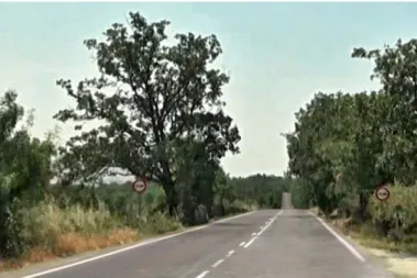
Roadside elements such as vegetation, traffic signs or buildings may be taken into account in the sight distance studies when using a DSM instead of a DTM. Regarding the roadside vegetation, trees and plants may reduce available sight distances, especial-ly when it comes to forests and denseespecial-ly wooded are-as. A sub-section of highway M-611 was selected to illustrate this issue. The design speed is assumed to be 40 km/h. A horizontal curve of radius 23 m is flanked by respective spirals and tangents. Figure 3 shows the actual view of a vehicle approaching a right curve, where a densely wooded area is found close to the inner roadside. In this case, both an air-borne DTM and an airair-borne DSM arranged in a 1-m. square mesh were used. The vehicle path was de-rived from cartographic data and was discretized into stations spaced 5 m apart.
Figure 3. Real view of curve where sight distance is limited by vegetation.
Figure 4 shows the sight distance graph superpos-ing the results of both a DTM and a DSM. When a DTM is used as input, the minimum available sight distance is 55 m (slashed line) whereas the corre-sponding to the DSM is 15 m (solid black line) around station 3150. The latter one is more in line with reality. This value would not comply with the stopping sight distance set at 50 m by the Spanish standard (Ministerio de Fomento 2016). Moreover, the available sight distance is reduced around 40 m all the way in front of the curve. This difference is highlighted in medium light green in Figure 4, which represents the sections that are seen when the input is the DTM whilst the study with DSM determined they cannot be seen. This example shows how
sig-nificant is the influence of vegetation by the road-sides by means of the choice of DEM.
In addition, a study carried out by the authors found that sight distance results using airborne DTM, airborne DSM and MMS DSM were all statis-tically significantly different (Castro et al. 2016). The differences were particularly relevant in sub-sections where the available sight distance was shorter.
Figure 4. Sight distance graph comparing results using DTM and DSM.
3.2 Hidden dips
Some combinations of horizontal and vertical align-ments might produce shortcomings in the driver’s perspective. Hidden dips are a common shortcoming on highways where the profile adjusts the terrain more strictly than the horizontal alignment. A hidden dip is produced where the driver is able to see two separate sections of the roadway while the stretch in between remains concealed. This typically occurs where a sag follows a crest curve on a rather straight horizontal alignment. It is essential to avoid poten-tially hazardous spots within the hidden section, such as intersections or unexpected changes in direc-tion. Moreover, these alignments may mislead driv-ers at the beginning of a passing maneuver, since on-coming traffic remains unnoticed in the hidden section.
The perspective shortcoming is first noticed at station 710. When the driver reaches station 725, the available sight distance is 380 m, a stretch of 240 m remains hidden, and a further segment is seen over again up to 905 m. The hidden dip ranges up to sta-tion 1060, totaling 350 m.
Figure 5. Real view of hidden dip on straight alignment
As this type of shortcoming may produce passing issues, the study of passing sight distance results in-teresting.In this section posted speed is 90 km/h. For this value, the current Spanish standard (Ministerio de Fomento 2016) demands a passing sight distance of 205 m along a section of 340 m or larger. Howev-er this threshold is exceeded along 165 m only. Thus passing should be prohibited all along the hidden dip range.
Figure 6. Sight-distance graph of hidden dip.
Furthermore, the German guidelines for the visu-alization of rural roads (FGSV 2008) describe the conditions under which a hidden dip is potentially hazardous for drivers, regardless of the design speed. Three conditions must be fulfilled simultaneously along a range of at least 60 m: The hidden sections must not spread out beyond 600 m from the driver, the hidden section has to cover more than 75 m and the depth of diving must exceed 0.75 m (hence the area in brown in Figure 6). These values are largely exceeded in the present case, reporting a measure of
risk exposure during passing maneuvers. Hence this spot may be potentially hazardous.
Similarly, the Swiss standard (VSS 1991) deter-mines the maximum distance to consider the reap-pearing section at 500 m for that speed. That occurs only from station 920, therefore the hazardous stretch would range 140 m.
3.3 Overhanging elements
In this case study, a cantilever traffic signal in a highway section was simulated. The aim is to ana-lyze the effect of the location of this signal on driv-ers sight distance, avoiding the problems associated to the use of a DSM. As in previous cases, a DEM is needed. In this case an airborne DTM arranged in a 1-m square mesh was utilized. In addition, the canti-lever traffic signal was modeled as a multipatch file taken from an open library (Trimble 2015). This multipatch was placed on 5 different locations (Ta-ble 1) along a section of highway M-104. The canti-lever traffic signal location covers exactly the width of the traffic lane where signing applies.
Table 1. Locations where cantilever signal was placed.
Location Station (m)
1 5260
2 5305
3 5400
4 5450
5 5630
The highway horizontal alignment is composed by a right horizontal curve, followed by a long tangent and a left curve. In the vertical alignment, there is a sag curve approximately on the middle of the tan-gent, between the two horizontal curves. The canti-lever traffic signal locations 1 and 2 are supported by the roadside on different spots of the right curve. Lo-cation 3 is at the beginning of the sag curve and lo-cation 4 is at the lowest point of the sag curve. Loca-tion 5 is between the sag vertical curve and the left horizontal curve. Figure 7 shows a 3D view made using ArcSCENE, where the different locations of the cantilever traffic signal considered are depicted. The right and the left horizontal curves overlap ap-proximately with two crest vertical curves.
The clearance height was 5.5 m, according to the current Spanish standard (Ministerio de Fomento, 2016) whereas the maximum height of the structure is 6.81 m. Moreover, such standard requires that the impact of gantries and cantilever signals on sight distance is checked.
parallel offset of 1.5 m from the highway centerline. Also, according to the same standard, target height was set at 0.5 m. Figure 8 shows the sight-distance graph when the calculation was launched without cantilever traffic signal. There is a first zone of shorter sight distance due to the first horizontal curve and the first crest vertical curve (minimum available sight distance of 115 m at station 4855). Then, the available sight distance increases until drivers approach the second horizontal curve and the second crest vertical curve (135 m of minimum sight distance at stations 5680-5715).
Figure 7. View in ArcSCENE of the cantilever traffic signal possible locations.
Figure 8. Sight-distance graph without traffic signal.
Figure 9 shows sight-distance graphs correspond-ing to location 1 of the cantilever traffic signal. In location 1, there are some lines of sight correspond-ing to driver location between stations 4940 and 5240 that intersect traffic signal post, but its effect is negligible. The cantilever signal itself has no effect on sight distance. Similarly, Figure 10 shows the sight-distance graph corresponding to location 4 of the cantilever traffic signal (near station 5450). Comparing Figures 9-10, it can be noticed that not only the cantilever traffic signal effect moves (due to the change of location) but also the non-visible area becomes larger. This latter effect is due to signal lo-cation at the lowest point of the sag curve. As a re-sult, the cantilever signal intercepts much more lines of sight, producing a more relevant hidden area.
Figure 9. Sight-distance graph corresponding to cantilever sig-nal at station 5260 (location 1).
Figure 10. Sight-distance graph corresponding to cantilever signal at station 5450 (location 4).
4. CONCLUSIONS
The proposed procedure demonstrates the potential and versatility of GIS in highway sight distance stud-ies. The inputs needed for the study, namely the driver’s eye height, the target height, the vehicle path and the elevation model were described. The im-portance of the resolution and nature of the DEM was particularly emphasized. To achieve precise re-sults, it is desirable to use high resolution models (1 node per m2). The outcome can be studied in detail with the aid of the tools and capabilities developed, including the sight-distance graph, line-of-sight pro-files and mapped features. Sight-distance graphs permit a detailed analysis of roadside elements which limit sight distance.
Throughout three case studies on in-service highways, the strengths and capabilities of the meth-odology were proved. To take account of the effect of roadside elements or vegetation on sight distance, DSMs must be used instead of a DTM. In particular cases, the reduction of available sight distance is es-pecially significant while considering these entities. The second case study showed how to detect and characterize sight-hidden dips. The parameters that may indicate the risk exposure of these sections, namely range, length of hidden section, dip depth minimum available sight distance and distance to reemerged stretch can be identified at ease with the tools provided.
Visible section Hidden section
A DSM leads to biased sight distance modelling where there are overhanging features because lines of sight are obstructed by the model surface even be-low the overhanging feature. The proposed GIS-based procedure may contemplate multipatch struc-tures to model them, overcoming the difficulties in-herent to the presence of overhanging elements. The third case study showed how to model properly a section with a cantilever traffic signal and its real impact on sight distance. The easiness to place mul-tipatch objects is an additional advantage provided by this procedure. This simplifies the simulation of object location to evaluate its possible effects on sight distance. Also, due to the availability of mul-tipatch datasets libraries, modelling effort is reduced.
Therefore the GIS based methodology presented is useful not only to study sight distance but also seek for potential safety issues though integrated analysis. Diverse operational factors such as accident data, traffic volume, operating speed and design con-sistency can be incorporated to locate and diagnose potentially hazardous spots or, eventually, to identify the factors involved in a particular accident.
5. ACKNOWLEDGEMENTS
The authors gratefully acknowledge the financial support of the Spanish Ministerio de Economía y Competitividad and European Regional Develop-ment Fund (FEDER). Research Project TRA2015-63579-R (MINECO/FEDER).
6. REFERENCES
Altamira, A. L., Marcet, J. E., Graffigna, A. B. & Gómez, A. M. 2010. Assessing available sight distance: an indirect tool to evaluate geometric design consistency. In Proceedings of the 4th International Symposium on Highway Geometric Design.
American Association of State Highway and Transportation Of-ficials (AASHTO) 2011. A Policy on Geometric Design of
Highways and Streets. Washington DC: AASHTO.
Campoy-Ungría, J.M. 2015. Nueva metodología para la obten-ción de distancias de visibilidad disponibles en carreteras
existentes basada en datos LiDAR terrestre. Doctoral
dis-sertation. Valencia: Universidad Politécnica de Valencia. Castro, M., Iglesias, L., Sánchez, J. A. & Ambrosio, L. 2011.
Sight distance analysis of highways using GIS tools.
Trans-portation Research Part C: Emerging Technologies, 19(6):
997-1005.
Castro, M. 2012. Highway design software as support of a pro-ject based learning course. Computer Applications in Engi-neering Education, 20(3): 468-473.
Castro, M., Anta, J. A., Iglesias, L. & Sánchez, J. A. 2014. GIS-based system for sight distance analysis of highways,
Journal of Computing in Civil Engineering, 28(3):
04014005.
Castro, M., De Blas, A., Rodriguez-Solano, R. & Sanchez, J. A. 2015a. Finding and characterizing hidden dips in roads.
Baltic Journal of Road and Bridge Engineering, 10(4):
340-345.
Castro, M & De Santos-Berbel, C. 2015. Spatial analysis of ge-ometric design consistency and road sight distance.
Interna-tional Journal of Geographical Information Science,
29(12): 2061-2074.
Castro, M., García-Espona, A. & Iglesias, L. 2015b. Terrain model resolution effect on sight distance on roads. Periodica Polytechnica: Civil Engineering, 59(2): 165-172.
Castro, M., Lopez-Cuervo, S., Paréns-González, M. & De San-tos-Berbel, C. 2016. LIDAR-based roadway and roadside modelling for sight distance studies. Survey Review, 48(350): 309-315.
Forschungsgesellschaft für Straßen- und Verkehrswesen (FGSV) 2008. Hinweise zur Visualisierung von Entwürfen für außerörtliche Straßen. Bonn: FGSV Verlag.
Forschungsgesellschaft für Straßen- und Verkehrswesen (FGSV) 2012. Richtlinien für die Anlage von Landstraßen. Bonn: FGSV Verlag.
Ismail, K. & Sayed, T. 2007. New algorithm for calculating 3D available sight distance. Journal of Transportation Engi-neering, 133(10): 572-581.
Jha, M. K., Karri, G. A. K. & Kühn, W. 2011. New three-dimensional highway design methodology for sight distance measurement. Transportation Research Record: Journal of the Transportation Research Board, 2262: 74-82.
Khattak, A. J. & Shamayleh, H. 2005. Highway safety assess-ment through geographic information system-based data visualization. Journal of Computing in Civil Engineering, 19(4): 407-411.
Kühn, W., Volker, H. & Kubik, R. 2011. Workplace simulator for geometric design of rural roads. Transportation Re-search Record: Journal of the Transportation ReRe-search
Board, 2241:109-117.
Larocca, A. P., Da Cruz Figueira, A., Quintanilha, J. A. & Kabbach Jr, F. I. 2011. First steps towards the evaluation of the efficiency of three-dimensional visualization tools for detecting shortcomings in alignment’s coordination. In Pro-ceedings of the 3rd International Conference on Road Safe-ty and Simulation.
Ministerio de Fomento 2016. Norma 3.1-IC: Trazado. Madrid: Ministerio de Fomento.
Roos, R. & Zimmermann, M. 2004. Quantitative methods for the evaluation of spatial alignment of roads, In Proceedings of the 2nd International Conference of Società Italiana di Infrastrutture Viarie (SIIV).
Topcon 2010. IP-S2 specifications. Available from Internet: <http://www.topcon.co.jp/en/positioning/products/pdf/ip_s2 .pdf>.
Trimble 2015. Sketchup PRO. Available from Internet: <http://buildings.trimble.com/products/sketchup-pro>. Vereinigung Schweizerischer Strassenfachleute (VSS) 1991.
Linienführung; Optische Aforderungen (SN-640140).