Imputation method based on recurrent neural networks for the internet of things

UNIVERSIDAD EAFIT

Engineering School

Imputation Method Based on Recurrent Neural

Networks for the Internet of Things

Graduation manuscript presented as partial requirement to obtain the

Master of Science in Engineering

AUTHOR:

Ing. Sebastián Rodríguez Colina

SUPERVISOR:

Ricardo Mejía-Gutiérrez, PhD.

Abstract

The Internet of Things (IoT) refers to the new technological paradigm in which sensors and common

objects, like household appliances, connect to and interact through the Internet. This new paradigm,

and the use of Artificial Intelligence (AI) and modern data analysis techniques, powers the development

of smart products and services; which promise to revolutionize the industry and humans way of living.

Nonetheless, there are plenty of issues that need to be solved in order to have reliable products and

services based on the IoT . Among others, the problem of missing data posses great threats to the

applicability of AI and data analysis to IoT applications. This manuscript shows an analysis of the

missing data problem in the context of the IoT, as well as the current imputation methods proposed to

solve the problem. This analysis leads to the conclusion that current solutions are very limited when

considering how broad the context of IoT applications may be. Additionally, this manuscript exposes

that there is not a common experimental set up in which the authors have tested their proposed

imputation methods; moreover, the experiments found in the literature, lack reproducibility and do

not carefully consider how the missing data problem may present in the IoT. Consequently, the reader

will find two proposals in this manuscript: i) an experimental set up to properly test imputation

methods in the context of the IoT; and ii) an imputation method that is general enough as to be

applied to several IoT scenarios. The latter is based on Recurrent Neural Networks, a family of

supervised learning methods which have excel at exploiting patterns in sequential data and intrinsic

association between the variables of data.

Keywords: Internet of Things, Incomplete Data, Missing Data, Imputation Methods, Recur-rent Neural Networks, Machine Learning.

Resumen

El Internet the las Cosas (IoT) es un nuevo paradigma tecnológico, en el cual sensores y objectos

comunes, como electrodomésticos, se conectan e interactúan a través de la Internet. Este nuevo

paradigma, de la mano con técnicas de Inteligencia Artificial (AI) y técnicas modernas para el análisis

de datos, hace posible el desarrollo de productos y servicios inteligentes; lo que promete revolucionar

la industria y la forma de vida de los humanos. Sin embargo, existen muchos problemas que deben

ser solucionados para poder contar con productos y servicios confiables basados en el IoT. Dentro de

estos problemas, el problema de los datos faltantes impide la correcta aplicación de modernas técnicas

the AI y análisis de datos en aplicaciones basadas en el IoT. Este escrito presenta un análisis del

problema de los datos faltantes en el contexto del IoT, así como métodos de imputatción actuales

propuestos a solucionar este problema. Del análisis se concluye que las soluciones actuales tienen

grandes limitaciones si se considera lo amplio del contexto de las applicaciones basadas en IoT. El

análisis también expone que no hay un marco experimental en común que pueda ser usado por los

diferentes autores, y que los experimentos encontrados carecen de reproducibilidad y no consideran

adecuadamente como el problema de los datos faltantes se presenta en el contexto en particular del IoT.

De acuerdo con lo anterior, este escrito presenta dos propuestas principales: i) un marco experimental

que permite evaluar adecuadamente los métodos de imputación que se pretendan evaluar en este

contexto; y ii) un método de imputación que es lo suficientemente general como para ser aplicado

en los diferentes scenarios del IoT. El método de imputación se basa en el uso de Redes Neuronales

Recurrentes, una familia de métodos de aprendizaje supervisado que ha mostrado un buen desempeño

explotando patrones de datos sequenciales y relaciones intrínsecas entre variables.

Palabras Clave: Internet the las Cosas, Datos Incompletos, Datos Perdidos, Métodos de Imputación, Redes Neuronales Recurrentes, Aprendizaje de Máquina.

State of Publications

During the development of this research project, I contributed to the following publications:

• Ruiz-Arenas, S., Rodríguez-Colina, S., Rusak, Z., Mejía-Gutiérrez, R., & Horváth, I. (2016).

Design of a Low-End Cyber-Physical System TestBed For Testing a Failure Diagnosis Algorithm.

In Proceedings of TMCE 2016 (pp. 1–9).

• Rodríguez-Colina, S., Zapata, C., Osorio-Gómez, G. & Mejía-Gutiérrez, R. (2017). An

Ex-perimental Analysis for Fault Detection and Diagnosis in the Internet of Things: A Home

Refrigerator Case Study. Accepted for oral presentation at IMECE, 2017. (*)

• Rodríguez-Colina, S., Mejía-Gutiérrez, R. (201X). Recurrent Neural Networks as Imputation

Method for the Internet of Things. Submitted toIEEE Internet of Things Journal (+).

(*) The presentation at this conference was accepted on July 2nd, 2017. However, due to financial

matters, it was not possible to present at the conference and the article was hence withdrawn on

August 10th, 2017. The article will be upgraded and submitted to an indexed journal.

(+) This article includes the most relevant content presented in this manuscript.

Nomenclature

Acronyms

AI Artificial Intelligence.

ANN(s) Artificial Neural Network(s).

AUEC Area Under the Error Curve.

CPS(s) Cyber-Physical System(s).

GRU Gated Recurrent Units.

IoT Internet of Things.

LSTM Long-Short Term Memory.

MAE Mean Absolute Error.

RNN(s) Recurrent Neural Network(s).

WSN(s) Wireless Sensor Networks(s).

Variables

ˆ

f Estimated function relating inputs to

out-puts.

ˆ

X A reconstructed matrix of data (without

missing values).

ˆ

x The predicted value of any variable in any

time step.

x Vector-value input or observation in a

data set.

D A data set.

T A data set used for testing supervised

learning models.

ε Inherent error between a particular

pre-diction and the corresponding true value.

d Number of variables in a data set.

f True function relating inputs to outputs.

i Index over the observations in a data set.

j Index over the variables in a data set.

k The probability that any variable (equal

for all variables) is missing in a Bernoulli

pattern of missing data.

l Index over the missing values in a data

set.

l O

Range of possible lengths of consecutive

missing observations in a row wise

miss-ing data pattern.

lO Range of possible lengths of consecutive

non missing observations in a row wise

missing data pattern.

m Number of missing values in a data set.

n Number of observations in a data set.

nan Indicator of a missing value.

P A vector of allPj.

v

Ph The higher missing rate for the column

wise missing data pattern.

Pj The probability that a particular variable

is missing in a Bernoulli pattern of missing

data.

Pl The lower missing rate for the column wise

missing data pattern.

Smiss The set of indices of the variables that will

be missing in the row wise missing data

pattern.

X A matrix of data without missing values.

Xnan _{A matrix of data with missing values.}

xj Single-valued input or observation of

vari-able.

Contents

1 Introduction 1

1.1 Background . . . 1

1.1.1 What is the IoT all about? . . . 1

1.1.2 The potential of IoT applications . . . 6

1.2 Research Problem . . . 7

1.2.1 Supervised machine learning basics . . . 7

1.2.2 Problem Statement . . . 8

1.2.3 Naïve approaches for the missing data problem . . . 10

1.2.4 Qualities of abetter imputation method . . . 11

1.3 Objectives . . . 12

1.4 Research Scope . . . 12

1.5 Research Justification . . . 13

1.6 Manuscript Organization . . . 14

2 Literature Review 15 2.1 Models of the Missing Data Problem . . . 15

2.2 Approaches to Impute Missing Data In the IoT . . . 20

2.2.1 Strong variable association . . . 20

2.2.2 Data from the IoT as time series data . . . 21

2.2.3 Other features of the reviewed solutions . . . 22

2.3 Concluding Analysis of the Literature Review . . . 23

3 Proposed Contributions 26 3.1 Simulation of Missing Data Patterns in the IoT . . . 26

3.1.1 Bernoulli independent missing data pattern . . . 27

3.1.2 Column wise pattern of missing data . . . 28

3.1.3 Row wise pattern of missing data . . . 29

Contents

vii

3.1.4 Estimating performance . . . 30

3.2 Supervised Learning for Imputation . . . 32

3.2.1 Exploiting relation between variables . . . 33

3.2.2 Exploiting temporal structure in the variables . . . 34

3.2.3 Regression methods . . . 34

3.3 Imputation method for the IoT . . . 35

3.3.1 Introduction to Recurrent Neural Networks . . . 36

3.3.2 Recurrent Neural Networks as an Imputation for data from the IoT . . . 39

4 Evaluation of RNNs as imputation method 41 4.1 Data Set 1: Individual Household Electric Power Consumption . . . 43

4.1.1 Evaluation of RNNs Hyperparameters . . . 43

4.1.2 Comparison with other imputation methods . . . 45

4.1.3 Summary . . . 49

4.2 Data Set 2: Air Quality . . . 49

4.2.1 Evaluation of RNNs Hyperparameters . . . 50

4.2.2 Comparison with Other Imputation Methods . . . 51

4.2.3 Summary . . . 54

4.3 Case Study: Impact of Imputation Methods on an IoT Application . . . 55

4.3.1 Online FDD of home refrigerators . . . 56

4.3.2 Effect of reconstruction error on classification accuracy . . . 58

4.4 A note on the variability of the AUEC metric . . . 61

5 Analysis and Conclusions 63 5.1 Analysis and Conclusions . . . 63

5.2 Further Work . . . 65

References 67

List of Figures

1.1 The number of transistors in integrated cirquits chips (1971-2011) (Roser and Ritchie,

2018) . . . 2

1.2 Wireless communication standards, their speed and usage (Shuang-Hua, 2014, pg. 2). . 2

1.3 Smartness hierarchy of IoT products . . . 4

1.4 Broad scale representation of the IoT. . . 5

1.5 Causes of losses in sensor data (Shuang-Hua, 2014). . . 9

1.6 Three situations in a classification task. (a) an example of a model ˆf learnt in a classification task for a bivariate data set, (b) a complete observation to be classified,

(c) an incomplete observation to be classified . . . 10

2.1 A picture of a part of the Intel Lab data set downloaded fromhttp://db.csail.mit.

edu/labdata/labdata.html. . . 18

2.2 A picture of a part of the Air Quality data set downloaded from UCI Machine Learning

Repository (http://db.csail.mit.edu/labdata/labdata.html). . . 19

3.1 Example of three Bernoulli missing data patterns generated by the procedure described

here. The gray areas represent missing values. . . 28

3.2 Example of three column wise missing data patterns generated by the procedure

de-scribed here. . . 29

3.3 Example of three row wise missing data patterns generated by the procedure described

here. . . 30

3.4 A graphical representation of a linear regression with three input variables. . . 36

3.5 A feed-forward neural network with three input variables and two hidden layers with

four and three units each. . . 37

3.6 A one-layer RNN. . . 38

3.7 A one-layer RNN that learns a mapping fromxttoxt+ 1. . . 39

List of Figures

ix

3.8 A RNN that explicitly uses a time window of data withp= 3 to predict the following

input vector. Note that the firstp−1 outputs are ignored. . . 40

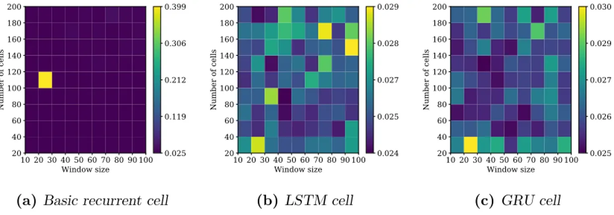
4.1 AUEC with respect to the number of nodes and length of time window. . . 44

4.2 AUEC with respect to the number of nodes. . . 44

4.3 AUEC with respect to the length of time window. . . 44

4.4 (a) Mean of the error against missing rate. (b) Violin plot of the AUEC for the three cell types, the red and green lines represent the mean and median values respectively. 45 4.5 (a) Reconstruction error against different values of missing rate of five methods. (b) AUEC. (c) Monte Carlo simulations testing the significance of the observed difference. 47 4.6 Results in a column wise pattern. (a) Mean reconstruction error. (b) Results of the two best performing methods. (c) Significance of the observed difference. . . 48

4.7 Results in a row wise pattern. (a) Mean reconstruction error. (b) Results of the two best performing methods. (c) Significance of the observed difference. . . 48

4.8 AUEC with respect to the number of nodes and length of time window. . . 50

4.9 AUEC with respect to the number of nodes in the air quality data set. . . 50

4.10 AUEC with respect to the length of time window in the air quality data set. . . 51

4.11 (a) Mean of the error against missing rate. (b) Violin plot of the AUEC for the three cell types, the red and green lines represent the mean and median values respectively. 51 4.12 (a) Reconstruction error against the missing rate. (b) AUEC . (c) Monte Carlo simu-lations testing the significance of the observed difference. . . 52

4.13 Results in a column wise pattern. (a) Mean reconstruction error. (b) Results of the two best performing methods. (c) Significance of the observed difference. . . 54

4.14 Results in a row wise pattern. (a) Mean reconstruction error. (b) Results of the two best performing methods. . . 55

4.15 Location of sensors in the system. . . 57

4.16 Location of sensors in refrigerators compartments. h1 andh2 refer to the height of the freeze and conservation area respectively. . . 57

4.17 A picture of the refrigerator used in the experiments. . . 59

4.18 Accuracy of two machine learning methods against the reconstruction error. (a) Imput-ing with last recorded value of every variable. (b) Imputation method based on PCA. (c) Imputation method based on RNNs with GRU cells. . . 61

4.19 Maximum standard deviation against the number of samples. (a) Household electric power consumption data set. (b) Air quality data set. . . 62

List of Tables

2.1 Exploited data relationships by articles. . . 24

2.2 Other characteristics of the reviewed solutions. . . 25

4.1 Probability that the difference in the median value of pairs of cells’ type is equal to or greater than the observed difference if the AUECs had come from the same cell type. . 46

4.2 Summary of the comparisons with the AUEC metric. . . 46

4.3 Summary of the experiments in a column wise pattern . . . 48

4.4 Summary of the experiments in a row wise pattern. . . 49

4.5 Probability that the difference in the median value of pairs of cells’ type is equal to or greater than the observed difference if the AUECs had come from the same cell type. . 52

4.6 Summary of the performance on the AUEC metric. . . 53

4.7 Summary of the experiments in the column wise pattern. . . 53

4.8 Summary of the reconstruction error in the row wise pattern of missing data. . . 54

4.9 Time for detection of most common faults in home refrigerators. . . 56

4.10 Label and location of sensors. . . 58

4.11 Classifiers’ performance on the training and test set, as well as the reconstructed data set by the five considered imputation methods. . . 60

Chapter 1

Introduction

1.1

Background

Computers are now much faster and smaller than they were twenty years ago: “current mobile devices

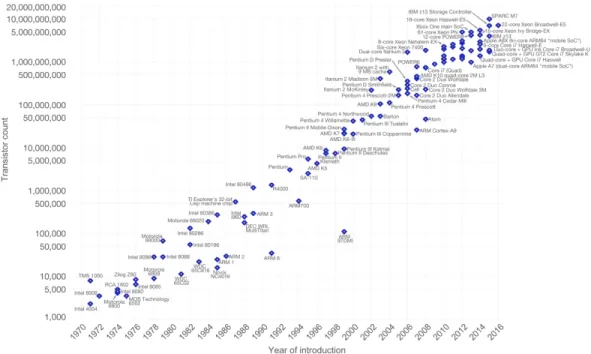
have more computation capabilities than the Apollo Guidance Computer” (Kaku, 2011, pg. 10). In

1965 Gordon Moore (Roser and Ritchie, 2018) predicted that by reducing transistors size, computation

would be exponentially cheaper and faster (see figure 1.1). Although it is widely argued that Moore’s

law is coming to an end of its validity (Simonite, 2016)—due to the upcoming of new computation

paradigms such as quantum computing—, it is good for showing out the impressive evolution of

computing for more than 40 years.

Wireless communication is also making progress. Several protocols and technologies have been

implemented widely on sensors, actuators and machinery. Every electronic device can currently be

connected to several others by means of different communication protocols (e.g. Wi-Fi, ZigBee,

Bluetooth, GSM; see figure 1.2) (Shuang-Hua, 2014).

As a consequence of such evolution of computation and communication technologies, a wide variety

of devices, including sensor-enabled smart devices and all types of wearables, connect to the Internet

and power newly connected applications and solutions (Gil et al., 2016). Such phenomena is what is

now known as the Internet of Things (IoT).

1.1.1

What is the IoT all about?

In a broad sense, the term IoT has been used to refer to a world where physical objects and beings, as

well as virtual data and environments, all interact with each other in the same space and time

(CERP-IoT, 2010). Such connectivity has the potential to power smartnessacross very different application

areas such as mobility, assisted living, environmental protection, agriculture, etc. And has also gain

2

Introduction

Figure 1.1:

Figure 1.2:

special interest from several governments (Friess, 2013).

1.1 Background

3

“The IoT is a concept and a paradigm that considers pervasive presence in the

envi-ronment of a variety of things/objects that through wireless and wired connections and

unique addressing schemes are able to interact with each other and cooperate with other

things/objects to create new applications/services and reach common goals. (pg. 7)”

It is usually said that the view expressed before is not quite accomplished and that there is still

plenty of research to be done. Up to now there is no unique solution for the development of the

IoT in terms of security, management and data analytics (Alaba et al., 2017; Earley, 2015; Tsai et al.,

2014). The data analytics side of the IoT is the responsible for bringing smartness (a.k.a cognitive

capabilities) into IoT products (F. et al., 2015). Such smartness has been consistently considered

the main objective of the IoT (Vermesan et al., 2013; Wu et al., 2014). This project is thus focused

on the data analytics aspect of the IoT, since the development of this aspect is crucial for the true

development of the IoT (Arsénio et al., 2014; Alam et al., 2016).

1.1.1.1

Applications

The way in which IoT applications can impact current products and services is by adding smartness to

them. As grouped by E. Porter and E. Heppelmann (2017) smartness in products comes in different

levels: monitor, control, analysis1 _{and autonomous reaction to the changes in environment. The}

distinction of these levels can be seen hierarchically in figure 1.3, and they are described as follows:

Monitoring

of alerts and notifications. For example consider the K’Track Glucose. It monitors glucose by a sensor

in a wearable watch; it can provide time series plot of the glucose levels; alerts of high levels and

reminders of times for medication. Monitoring applications may make use of signal processing to

correct errors from sensors.

Controlling

can change lighting conditions based on user instructions via smartphone. Users can also provide

timers and set alarms. However, industrial or more complex applications (see the Roomba robot)

require more control than it is provided by most platforms; it is therefore, typical to use cascade

controls where more complicated and real-time algorithms are applied locally, whereas parametrisation

of such algorithms takes place remotely.

Analysis

theconstrained world of the applications and improve the way the product gets things done. It can

1_{The original word used by the author was optimisation, but the word analyse seems to be more suitable}

4

Introduction

also help maintenance by providing product diagnostics based on data. Applications at this stage are

simply a help for people and there is no autonomy exhibited.

Autonomy

is what products exhibit when they adapt without human intervention to different scenarios or user

preferences.

Figure 1.3:

There are several platforms that allow applications with any level of smartness to be developed

more easily. Every IoT platform allows the monitoring stage of development (see for example Ubidots).

However not all IoT platforms support the later three levels (ThingSpeak, ThingWorx, AWS IoT, IBM

Watson IoT and Google IoT Solutions are platforms that do)2_{. It is worth mentioning that none of}

these platforms provides support in the form of plug and play solutions —besides monitoring and

very simple control— they rather provide access to the tools for development of the other levels of

smartness in the form of software libraries.

1.1.1.2

Prototypical architecture

Figure 1.4 shows a typical representation of the IoT. It shows some application areas and how they

integrate with the Internet. Some domains such as smart homes (Alaa et al., 2017) would need a

gateway3 _{to connect to the Internet, whereas some objects orThings in other domains may connect}

2_{https://thingspeak.com/apps, https://www.thingworx.com/, https://aws.amazon.com/}

iot-platform/, https://www.ibm.com/internet-of-things/and https://cloud.google.com/solutions/ iot/

3_{A device that connects two systems that use different protocols (IEEE Standard Glossary of Computer}

1.1 Background

5

directly.

The gateway allows wired and wireless connections between objects inside a small network such

as the one in a smart home environment; however, connections are usually wireless, which allows a

dynamic distribution of objects. The last description is what is known as Wireless Sensor Networks

(WSN) (see Shuang-Hua, 2014, for details). Gateways allow independent environments to have access

to a bigger network to expand their capabilities for computation and perform analytics in a larger

scale, in which developers can include data from all those independent environments. In contrast,

real-time (but limited) decisions require some processing to be made locally (Arsénio et al., 2014).

Figure 1.4:

In the cases of Smart Factory and Smart Logistics shown in figure 1.4, other terms have also

emerge: Cyber-Physical Systems (CPS) and Industry 4.0. All these terms share a lot of or make use

of the IoT, but their subtle differences are not relevant to understand this manuscript; please refer

to Henning et al. (2013); Henning, Kagermann. Wolfgang, Wahlster. Johannes (2013) for a deep

description about these.

As the amount of objects connected to the Internet grows, complicated applications start to emerge

and some previously unrelated objects start to make sense when used together (e.g. factories can

adjust production in connection to real-time logistics by considering supply and market predictions;

see Stolpe, 2016). Such applications rely on data analysis being performed remotely; furthermore,

local computer power is usually very limited and applications may share different sources of data

6

Introduction

to achieve a desired application (e.g. predictive maintenance, real-time route planing, etc.).

1.1.2

The potential of IoT applications

It is clear that the era of the IoT facilitates data extraction across several domains. Thus, there is

a huge opportunity to extract knowledge from IoT applications. Moreover, the IoT relies on data

analysis to exploit its true potential; leading to innovative new business models, products and services

(Stolpe, 2016). It is not just about connectivity, but about how such connectivity can be used to

enhance products’ behaviour and learn from their context (Stolpe, 2016; Tsai et al., 2014).

In the following paragraphs, I present the hypothetical evolution of a bike rental system. It

should be noted that at any stage, other enhancements could take place. However, the presented ones

are specially chosen to emphasize the impact of using data analysis to exploit the true potential in

IoT products.

IoT for remote monitoring.

interesting to add a GPS to every bike in the rental system. The location of each bike can then be

traced by users or administrators via a map interface on a web page. Knowing the location of bikes

will allow users to decide which station to go for a bike; will help administrators to define new stations;

and might prevent a bike from being stolen.

IoT for interaction with the system.

administrators of the rental system of bikes leaving a predefined area. It could also respond to user

queries about the availability of bikes near his current location. At this stage, people would not have

to see a map for themselves, they can just ask queries or subscribe to notifications.

IoT to extract knowledge from the system.

guarantee that, at any time, there is a certain amount of bikes available. This can be done with data

analysis techniques tailored to predict the demand of bikes based on the time of the day and the day

of the week. Predictive maintenance and fault detection of every bike can also be developed by the

use of AI and data analysis.

Please refer to Stolpe (2016) for an elaborated description on how manufacturing; transportation

and distribution; energy and utilities; public sector; and health care and pharmaceutical; can benefit

1.2 Research Problem

7

1.2

Research Problem

As said before, the focus of this work is on the analytics side of the IoT . Analysis of the data from

the IoT can only be carried out by what is known as machine learning or data mining4 _{(Tsai et al.,}

2014; Alam et al., 2016).

Machine learning, a form of AI,is a very active area of research which deals with finding patterns

in data, where data can be anything from pictures or words to sensor readings. These patterns can be

used for very different tasks, for example, they are the driving force of autonomous driving systems

(Aeberhard et al., 2015; Ziegler et al., 2014) and translation systems (Singh et al., 2017). Systems

built using machine learning show a great level of adaptation to the environment presented to them

in terms of data.

Machine learning can be broadly classified into three types of algorithms:supervised,unsupervised

and reinforced. Here I introduce some fundamental concepts of supervised learning. The following

provides only enough material to understand the research problem of this project, but its scope is

very limited in terms of all the possibilities provided by machine learning. Interested readers are

encouraged to review and expand the subject in any or some of the following: Izenman (2008); Hastie

et al. (2009); P. Murphy (2012); Bishop (2006). I also take this opportunity to introduce some useful

notation.

1.2.1

Supervised machine learning basics

The idea of supervised learning is to give computers examples of the task a human want them to

perform. Such procedure is calledtraining. The computer is then left to perform the task by itself,

which may be referred as theoperation time oroperation stage.

The task is always to predict the value of a variableybased on a vectorx. In general,xandycan be any type of data, but they are always defined in terms of categorical variables (i.e. variables with

a finite set of values like people’s gender and whether a household appliance such as a refrigerator is

on) or continuous variables5 (e.g. people’s height and the temperature of water). The task mentioned

above is calledclassification ify represents a categorical variable, whereas it is calledregression ify corresponds to a continuous variable.

Usually, training means to feed alearning algorithm with a number of examples from atraining

data set D={(xi, yi)}ni=1, where nis the number of training examples; every xi is ad-dimensional

input vector called aninstanceor anobservationrepresenting sensor readings; and finally,yirepresents

a particular example of what we want the computer to output from the input vector.

4_{In this work, the term data mining will not be used. Please refer to Izenman (2008, chap. 1) for clarification}

on the difference (if any) between the two terms.

5

8

Introduction

The scope of IoT applications is so vast that there could be applications requiring xandy to be a mixture of categorical and continuous variables; nonetheless, it is usually required that every pair

(xi, yi)∈ Dhas the same structured format. Every dimension along thed-dimensional input vector is

called afeatureor avariable; thus, everyxi(boldface and indexed byi) has the same set of variables.

Each of the variables are denotedxj (regular type face and indexed byj) forj∈ {1,2, ..., d}; unless I

refer to the value of the variable in a particular observation, in which case I writexi,j.

For all practical purposes, a learning algorithm is a computer procedure which aims to find a

functionf called themodel. The model refers to a correspondence between everyyi and everyxi. In

other words, supervised learning is an attempt to findf such thatyi=f(xi) +εi∀i, whereεi is the

error between a particular prediction by the model and the real observed value. I omit the index i and refer to such correspondence asy=f(x), when the interest is not in a particular pair (xi, yi).

In practice, after training, there is no way of knowing whether the algorithm has found the exact

f; therefore, the algorithm is said to find an approximate model ˆf such that y ≈ fˆ(x). This ˆf is then evaluated using a test set. The test set T can be said to be every available pair (xi, yi)∈ D/ .

The performance of the learnt model ˆf is estimated by comparing yi with ˆf(xi) for every xi and yi

available inT. Once a good performance measure has been achieved, the model is set on operation:

it will be provided with new x values and humans or other computational systems will rely on the model’s estimated value ˆf(x).

Most of the techniques for supervised learning impose little or no assumptions about xandy to be able to make a good estimate off. Moreover, regardless of violations to the assumptions imposed in the mathematical derivation of the learning algorithms, the resulting models are judged based on

their performance on the test set. On the other hand, it is required that all possible xi in D or T

or in operation time have the same set of features (format); the value that every variable takes for a

particularxcan obviously be different.

1.2.2

Problem Statement

As said by Stolpe (2016), IoT-enabled devices will become part of a highly dynamic network, in

which devices can come and go from time to time. For illustration, consider the bike rental system

described in section 1.1.2. If a sensor inside a particular bicycle is out of battery, its value would not

be recorded for a certain period of time. If a supervised learning-based application relies on the value

of that sensor (and others), it would not work until the sensor has enough power to transmit its value.

Mathematically, this means that some of the xj may be missing from some of the x (observations),

making the model ˆf useless (Yan et al., 2014). Figure 1.5 shows more reasons that may cause missing one or many variables from any observation.

1.2 Research Problem

9

Figure 1.5:

have less elements from what is expected. In this new scenario, an observation can be as in expression

1.1, where nanmeans the absence of a value (i.e. a missing sensor reading).

x=hx1, nan, . . . , xj, . . . , xd−1, nani. (1.1) Therefore, there is a need for IoT applications to adapt to such situation and keep responding

properly. To elaborate on the limitations of current methods on such situations, consider the following

example.

Suppose a classification task is being performed based on sensor readings from a network of

two fixed sensors. This time, the task consist of identifying two groups of observations, which may

represent optimal and suboptimal operation of a household appliance. Once training has been carried

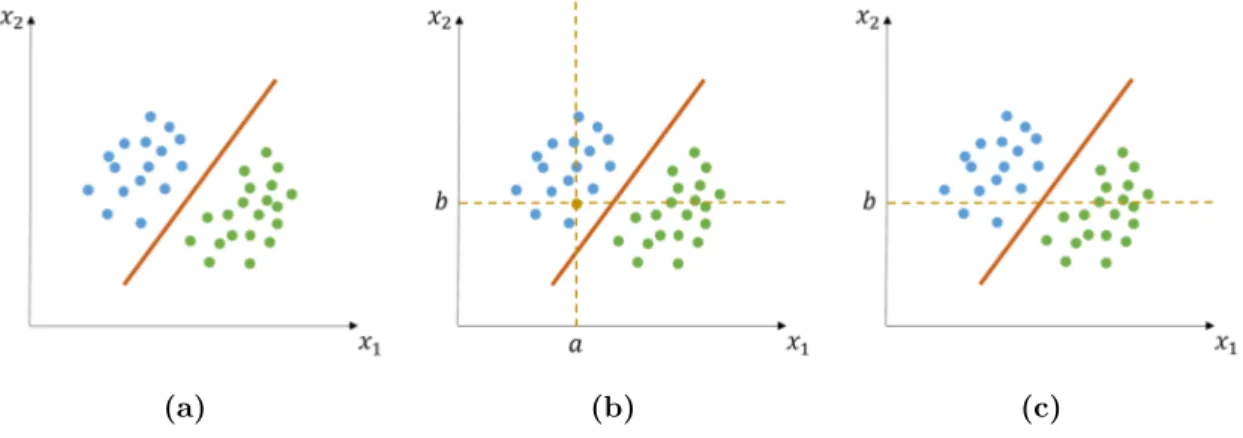
out, the training data set and the model ˆf could look like illustrated in figure 1.6a, where the orange line represents the learnt model that can distinguish between the two groups of observations.

In a regular situation, a new observationx=hx1=a, x2=biarrives to the data centre and it is easy to see its location relative to the model (see figure 1.6b). This location is what defines whether

the model say it corresponds to a group or the other.

Sometimes, however, a sensor may be under maintenance or could have gone out of range. In

such condition, a particular observation arrives at a data center as hx1 =nan, x2 =bi. Classifying such observation becomes a difficult task (see figure 1.6c). This situation has been named as the

incomplete dataor missing dataproblem: observations in a data set may contain values that are

10

Introduction

(a) (b) (c)

Figure 1.6:

1.2.3

Naïve approaches for the missing data problem

The missing data problem is present in several other fields, like medicine (Barclay et al., 2018; Bell

et al., 2014) and sociology (Ellison and Langhout, 2017). Therefore, solutions to this problem have

been proposed (Little and Rubin, 2002) that are not tailored to the specific needs of the IoT. Here, I

present some of those solutions together with an explanation on why those approaches are not suitable

for IoT applications.

1.2.3.1

Omit features or observations

In social experiments, an interview is applied to a big enough sample set (size of the sample set will

depend on the size of the population). Even if the interviewer properly selects the questions to be

included in the interview, there might be some people that for several reasons do not provide answers

for some of the questions. In such cases, data analysis of the interview’s results can require handling

of missing data in the following way:

• If there is an insignificant number of interviewees which has avoid answering one or many of the

questions, the interviewer can simply delete such observations (i.e. pretend that the interview

was applied to less people). Statistics derived from such a treatment may be less significant.

• Delete all features where missing values are present, which may cause the interviewer to answer

a different set of questions (from the full set of questions that was originally of interest) about

the population.

Consider the case of applying the first strategy in the context of the IoT: during training time, it

may not be harmful to omit some observations (i.e. some training examples), which is specially true

1.2 Research Problem

11

data problem may happen for long periods; thus, a system that relies on machine learning predictions

becomes unresponsive or useless if the first strategy is adopted.

During training time, the second approach may cause the learnt model to be inaccurate, because

there is not enough information to build an accurate one: the modelsunderfitthe data. Moreover, in

operation time, the system would be useless, as shown in figure 1.6c.

1.2.3.2

Imputation based approaches

A wiser and more useful way to deal with the missing value problem is to replace (impute) a missing

value with some estimation for that value; nevertheless, imputation should be applied carefully. Here,

I show naïve approaches, but I discuss more elaborated and applicable approaches to imputation in

the IoT in Chapter 2.

Carry out last observed value

small number of observations and features that may be missing; and when those features relate to time

series data (such as sensor data), is to use the last observation of a variable as the value to impute.

However, such estimation of a missing value results inappropriate when there are subsequent missing

values of the same variable.

Imputation of the average values

the corresponding average value observed in a training set or a certain period of time. However,

the context in which it is applied may have several different operation modes; thus, the mean of a

certain variable during a period of time may be a bad estimate of that variable in a latter period (e.g.

the mean of the temperature outside a home refrigerator is usually a lot higher at midday than at

midnight).

1.2.4

Qualities of a

better

imputation method

The main subject of this project is to work towards the development of better imputation methods

for the context of the IoT. This would require a consideration of the following:

I. Since the mechanisms that generate the missing data problem are different across different

domains, more suitable imputation methods for the IoT should take into account a precise

description of the several mechanisms that would lead to missing data problems in the IoT.

II. As explained in section 1.1, IoT applications may be the result of inputs of data from different

environments and therefore, proper imputation methods should beapplicable to a great variety

of cases, by keeping assumptions about the data as little as possible.

III. Imputation methods shouldadapt to changes in the process generating data, that is, when the

12

Introduction

IV. Since applications are expected to run smoothly during operation time, imputation methods

shouldprovide estimates as they are needed in order to avoid bottle necks.

The above brief description of supervised learning, thus, seems like a good starting point for a

solution items II and III, since it has been applied to a great variety of cases and have been shown to

extract what is relevant from the data instead of imposing conditions on it.

1.3

Objectives

As a consequence of the analysis presented in Section 1.2, I now present the general and specific goals

pursued during this research project:

General objective:

To propose an imputation method for Internet of Things applications, through the use of supervised

learning, to make accurate predictions of the missing values.

Specific objectives:

(I) To analyse how the problem of missing data problem presents in the IoT, in order to build a

model of the problem and appropriately judge imputation methods in this context.

(II) To propose an imputation method to solve the missing data problem in the IoT.

(III) To evaluate the proposed method by comparing it with other solutions in situations that may

be encountered in the IoT.

(IV) To evaluate the impact of different imputation methods (i.e. their performance) on the reliability

of a smart application in the IoT.

1.4

Research Scope

Several aspects of application of advanced data analysis to the IoT have been described in many works

such as Arsénio et al. (2014); Stolpe (2016); Gil et al. (2016); Wu et al. (2014). Among other aspects,

there is the need to handle the gigantic amount of data that can be generated by the IoT, both in

terms of features and observations; the noisy nature of data coming from sensor networks and the

speed at which this data arrives to an analytics server; however, I will only consider the situation

presented in Section 1.2.

The missing data problem could also be addressed by constructing better communication protocols,

designing better sensors and platforms that integrate all available data. Those solutions are very

1.5 Research Justification

13

which very often operate under different protocols. Therefore, I will not consider those approaches in

this work.

In the rest of this project I will assume that there is a maximum number d of variables to be considered (i.e. whether missing or not, the number of variables is defined from the beginning).

Observations may have a numberd∗≤din the case of missing values. However, I will not consider the case of a growing network of devices (i.e. d∗≥d). Traditionally, it will cause constant reformulation of the imputation method, as well as data analysis algorithms, but it would add a lot of computational

complexity. This is a relevant challenge for the development of the field and further work should

definitely consider it.

The problem of missing data is not only present in the context of the IoT. It is also present, for

instance, in medicine (Masconi et al., 2015; Netten et al., 2016) and genetics (Eaton et al., 2017).

However, very often the proposed solutions and methodologies are developed for their special context.

Therefore, I developed the state of the art with solutions that were proposed in the context of the

IoT.

1.5

Research Justification

Earley (2015) highlights that organizations still have the challenge of understanding how the inclusion

of machine learning in the IoT can add value to their businesses; it is a fact in the academia world

though. Wu et al. (2014) argued that “without comprehensive cognitive capability, IoT is just like an

awkward stegosaurus: all brawn and no brains.”6. So integration of machine learning to the IoT is

required to fulfill its expectations.

Alam et al. (2016) evaluated eight machine learning algorithms and concluded that their

applica-tion to the IoT showed promise; however, they evaluated the algorithms based on training time and

prediction accuracy. In contrast, several authors have argued that traditional methods for machine

learning should be adapted to face all the needs of IoT applications (Stolpe, 2016; Tsai et al., 2014; F.

et al., 2015) and highlight the importance of handling missing data as it is ubiquitous in the context

of the IoT.

Missing data in the IoT can be caused by physical limitations or by design (Tsagkatakis et al.,

2016; Bijarbooneh et al., 2016). Interference, node/link failure, physical obstacles, environmental

change, unstable communications, unreliable sensors, etc. make observations unpredictable (Nower

et al., 2015; Yan et al., 2014; Sujbert et al., 2016; Zhao et al., 2016) by simple approaches. Using

naïve approaches can lead to faulty conclusions and predictions from data (Srinivasan et al., 2016).

As I show in Chapter 2, current solutions to the missing data problem are limited in its

imple-6

14

Introduction

mentation, since they are based on assumptions that are do not always apply to the great variety of

IoT applications. For instance, some solutions assume a particular probability distribution generating

the data and the missing values; others rely on manually chosen parameters. The imputation method

I propose in Chapter 3 is consistent with the qualities expected from imputation methods in the

IoT, so this project has considerable practical relevance. Moreover, the imputation method shown in

Chapter 3 is intended to help developers of IoT applications by providing an imputation method that

is applicable to a great variety of cases due to the comparably limited assumptions in its conception.

This project is also relevant from a theoretical perspective, because by building a model of the

missing data problem in the IoT (see Section 3.1), fellow researchers will be able to reason about

imputation methods that will be more suitable to the context of the IoT. Building this model also

contributes in the definition of proper experimental studies that will help to select from different

existing imputation methods.

1.6

Manuscript Organization

The rest of this manuscript is organized as follows. In Chapter 2 I present the relevant state of the art

in imputation methods proposed in the context of the IoT. Chapter 2 also shows approaches to model

the missing data problem and the way in which proposed imputation methods have been evaluated.

Afterwards, Chapter 3 shows the imputation method I propose, together with three models of the

problem of missing data in the IoT and their use to test imputation methods. I performed several

experiments to test the validity of the proposed method of imputation and show their results in

Chapter 4; the same chapter also presents the impact that different imputation methods have on the

quality of a smart application. Finally, I present an analysis of the results of this research project and

Chapter 2

Literature Review

Since the problem of missing data in the IoT has been reported significantly (Tsagkatakis et al., 2016;

Zhao et al., 2016), several authors have proposed solutions. In this chapter I show:

• Approaches to model the missing data problem and why this is important (see Section 2.1).

• Current solutions to handle the missing data problem (i.e. imputation methods), their main

features and limitations (see Section 2.2).

Often, the terms IoT, CPS and WSN appear together in scientific literature. Moreover, the missing

data problem has been reported together with any (or more) of those terms, and the choice between

terms is usually defined by the context of the authors. Therefore, the solutions I present in this

chapter have been proposed in any of those terms. Nevertheless, I omitted solutions that were heavily

dependant on information not available at the application layer of Figure 1.4 (e.g. signal strength in

wireless communications). It is important to note that, on the application level, developers may only

have their data and some information of its context.

In the end of this chapter, Section 2.3 presents the conclusion of what I found in the previous two

aspects of the state of the art and highlight what is missing in current practices from the perspective

of the IoT.

2.1

Models of the Missing Data Problem

Before describing solutions (e.g. imputation methods or algorithms) to the aforementioned problem

and their limitations, it is first necessary to define the model of the problem itself. Such a model can

be used to properly understand solutions and estimate some measure of their quality. Let me first

introduce some notation so that the following discussion can be easily understood.

16

Literature Review

x1,1 x1,1 . . . x1,j . . . x1,d x1,d

x2,1 x2,1 . . . x2,j . . . x2,d−1 x2,d

..

. ... . .. ... . .. ... ...

xi,1 xi,2 . . . xi,j . . . xi,d−1 xi,d

..

. ... . .. ... . .. ... ...

xn−1,1 xn−1,1 . . . ... . . . xn−1,d−1 xn−1,d

xn,1 xn,1 . . . xn,j . . . xn,d−1 xn,d

                  ,

where the index iis used to denote different observations,nis the number of observations andd is the expected number of variables per observation. Such data set is namedcomplete when there is

not a singlenanin it. In contrast, anincompletedata set is one with at least one nanin it:

Xnan =

                

nan x1,2 . . . x1,j . . . nan x1,d

x2,1 x2,2 . . . x2,j . . . x2,d−1 x2,d

..

. ... . .. ... . .. ... ...

nan nan . . . xi,j . . . xi,d−1 xi,d

..

. ... . .. ... . .. ... ...

xn−1,1 nan . . . xn−1,j . . . xn−1,d−1 nan

nan xn,2 . . . xn,j . . . xn,d−1 xn,d

                 .

Finally, areconstructed data set ˆX is one on which an imputation method has successfully been applied, therefore, it has no missing data in it. I do not use the word successfully as an indication of

the performance of such imputation method; it rather means that ˆX has no missing values.

The most commonly accepted way to assess the quality of an imputation method (see Liu et al.,

2012; Nower et al., 2013; Pan et al., 2014; Yan et al., 2014; Li et al., 2015; Tsagkatakis et al., 2016;

Zhao et al., 2016) is the following:

1. Take a complete data set.

2. Generate an incomplete data set by removing some entries of the one measured in the previous

step, following amodel for the process that causes missing data.

3. Impute with the imputation method to be tested, creating a reconstructed data set.

4. Compute thereconstruction error.

The reconstruction error (see Tsagkatakis et al., 2016) can be defined as any error measure between

X and ˆX. One can say that imputation methods try to predict values xi,j for all pairs (i, j) for

which the entry of the matrix X in position (i, j) is nan. Such predictions are labelled as ˆxi,i. The

2.1 Models of the Missing Data Problem

17

Not all authors have computed the reconstruction error in the same way, and there seems to be no

preference among the different possibilities. I adopted the Mean Absolute Error (MAE), computed as

m

P

l=1

|xl−xˆl|

m ,

wheremis the total number of missing values andlis just an index over the whole list of entries with missing values. For an argument about why this measure is preferred, see Willmott and Matsuura

(2005).

The most significant difference I found in different works is the model the authors used to generate

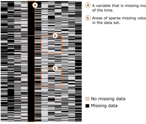
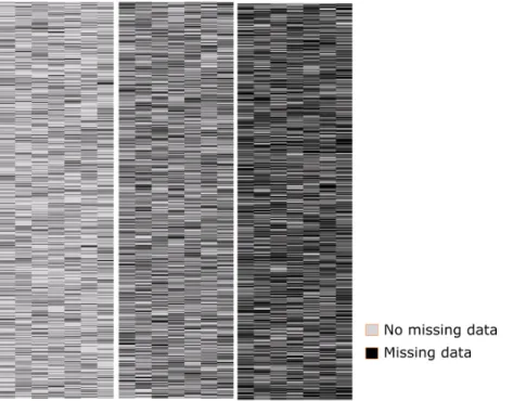
the incomplete data set. To have an idea of the type of results a model should produce, figures 2.1

and 2.2 show a picture of two public data sets that have been exposed in several articles regarding

(see e.g Pan et al., 2014; Yan et al., 2014) the missing data problem. In each of these figures the

gray parts represent a non missing values and the black ones represent missing values or consecutive

missing values an the boxes highlight some patterns of interest. The reader is reminded that columns

represent variables and rows represent observations.

Yan et al. (2014) defines three classes of missing data problems: i) when there is only one variable

and an observation is missing at rowibut neither rowi−1 ori+ 1 are missing; ii) when there is only one variable and an observation is missing at rowi and either rowi−1 ori+ 1 is not missing; and iii) when there are two or more variables and there is a missing value at any position (i, j).

The first two cases do not generalize to the case of missing data in the IoT for two reasons: i) the

number of variables in the IoT can be huge, ii) there can be subsequent missing values due to sources

of data being out of range or out of power (Shuang-Hua, 2014). The last one has been adopted by

other authors and is also expected in reality (see box b in figure 2.1), but the above description is

certainly not concrete (i.e. there are a lot of situations that fit the description). Therefore, such

description cannot be translated into a computer code that would consistently produce incomplete

data sets. Descriptions of this type are found also in other articles (e.g. see Zhang and Yang, 2014;

Pan et al., 2014; Zhao et al., 2016).

In the case of only one variable Sujbert et al. (2016) also showed three models for missing data1

i) for every i ∈1,2, ..., nthere is the same probability of observation i not being recorded (random independent data loss); ii) divide data into blocks and for every block there is a probability of that

observation block being recorded (random block-based data loss); and iii) there are two probabilities

of an observation not being recorded, use one of them when the previous observation was recorded

and the other one otherwise (Markov model-based data loss).

If one considers a generalization of the first two models to any number of variables, it is clear that

such models can generate patterns like some areas of figures 2.1 and 2.2. In contrast, although the

1

18

Literature Review

a A variable that is missing most of the time.

Areas of sparse missing values in the data set.

b a

b

b

No missing data

Missing data

Figure 2.1:

third model makes intuitive sense from the perspective of sensor networks, the authors did not show

the kind of pattern it would generate.

Li et al. (2015) propose two models: i) repeatedly choose a random time (row) and a random

variable (column) (Random Missing Pattern); ii) after a certain number of rows of complete data, the

rest will be completely missing in all variables (Consecutive Missing Pattern).

In this case, the first pattern seems very reasonable when looking into boxbof figure 2.1, whereas

the second seems to recreate some parts of the pattern shown in figure 2.2. Nevertheless, none of these

models would cover the fact the missing data mechanism may affect some variables more than others

(see box b of figure 2.2) or that blocks or missing and non missing data may alternate as shown in

boxa of figure 2.2.

Finally, Kong et al. (2013) defined four independent patterns of missing data: i) Element Random

Loss, in which missing values are sparse across the data set; ii) Block Random Loss, in which the

2.1 Models of the Missing Data Problem

19

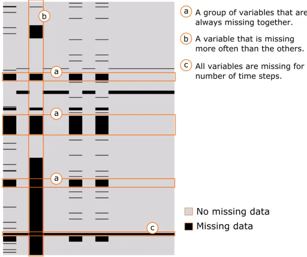
a

a

a b

c

a A group of variables that are always missing together.

A variable that is missing more often than the others. b

All variables are missing for a number of time steps.

c

No missing data

Missing data

Figure 2.2:

iii) Element Frequent Loss, in which some variables are missing intermittently; and iv) Successive

Element Rows, in which from a certain moment, some variables are lost and are not observed thereafter.

This definitions were made by an analysis performed on real data sets, and they showed examples of

these patterns. Indeed, looking at figures 2.1 and 2.2 reveals that the description match some areas of

those figures. However, they did not provide precise descriptions to simulate such patterns. Moreover,

as I show in Chapter 3.1, this patterns can be summarized into more concise descriptions for ease of

simulation.

Other works did not emphasize the way in which authors modelled the missing data problem

and simply mentioned that some entries, usually specified as percentage of the whole data set, were

removed (e.g. see Pan et al., 2014; Zhao et al., 2016). An unfortunate consequence of such a poor

model specification implies that different experimental results are not reproducible across research

20

Literature Review

becausethey may not reflect the reality of missing data in the IoT.

Another problem I found is that, although some authors tested their methods against others (see

Nower et al., 2015; Tsagkatakis et al., 2016), the relative difference between competing imputation

methods was not properly estimated. Usually, the authors made reported their results on simple plots

of an experiment, which raises the question of whether the difference they found was statistically

significant. Therefore, there is a need for quantitative measures that allow proper hypothesis tests

between competing imputation methods to be carried out.

2.2

Approaches to Impute Missing Data In the IoT

In the context of the IoT there have been two main assumptions that underlie all the imputation

methods that have been proposed:

• There is a strong association between the variables of a data set; in other words, the values that

a variable may have are greatly influenced by the values of other variables in the data set (e.g.

when the temperature in a room increases, the humidity may do as well).

• Data from the IoT is time series data, which means that all rows in a data set were collected

sequentially, meaning that if rowiwas collected at timet, rowi+ 1 was collected at timet+ 1. For this reason I often uset instead ofi.

In what follows, I describe those assumptions in detail and show which of the review imputation

methods relies on them. Finally, also describe a set of conditions that the authors defined so that

their methods would work (e.g. assumptions about the data).

2.2.1

Strong variable association

On the sensor level, it is a common practice to locate several nearby sensors measuring the same

variable, which results in a data set that contains copies of the same variable. In a data center this

can be exploited by combining those measured variables into a single one and therefore one can safely

ignore the missing value.

This simple strategy is not always possible and it is extended by Liu et al. (2012). For a missing

value coming from a corresponding sensor, their approach was to compute a missing value based

on the real distance between theneighbouring sensors. Likewise, Nower et al. (2013) computed the

imputed value based on the neighbouring sensor, which measures the same variable, for which there

is the highest correlation coefficient.

What is common in these approaches is that the authors assumed that nearby sensors were sensing

the same variable, which is the same as saying that there is aspacial relation between the variables.

2.2 Approaches to Impute Missing Data In the IoT

21

a dataset is expected to have information from several independent WSN and other sources of data.

The previous assumption is often relaxed in other works, like Pan et al. (2013, 2014) that, although

they expressed their ideas based on the spatial association between the variables, the values produced

by their methods are the result of linear regression models with respect to the variables without

missing values, which work even if the variables of the model do not represent the same physical

parameter.

As opposed to assuming a linear relationship between the variables, other authors assumed anon

linear relationship between the variables in a data set. For example, Gao et al. (2012) used a Support

Vector Regression with a non linear kernel (see Vapnik, 1998, ch. 11) to estimate the values of the

variables with missing values, based on the variables that do not have missing values.

Although the previous non linear approach is, in a sense, more general than the linear one, the

choice of the kernel imposes certain form of relation between the variables (i.e. the one defined by the

kernel). In contrast, Zhao et al. (2016) proposed the use of Stacked Autoencoders (see Goodfellow

et al., 2015, ch. 14), which can be trained to produce the most suitable form of non linear relationship

between the variables, while producing a lower space representation of them (i.e. a representation of

the same data with a reduced number of variables). Their method uses such a lower representation

to produce cluster of data points and change their imputed value until the clusters are stable.

2.2.2

Data from the IoT as time series data

A time series is defined as a set of quantitative observations arranged in chronological order

(Kirchgäss-ner et al., 2013). In most cases, such observations are equally separated by discrete time steps. Since

the IoT collects data from a multitude of sensors, it is plausible to have all this data arranged properly.

In fact, this property has been exploited by several authors assuming some type of relationship

(e.g. linear or non linear) between a variable and the same variable a few time steps ahead. Bylinear

I mean that the value of a variable at timetis predicted as a linear combination of the previous values at other times, plus some other terms that do not include the variable. In contrast, I refer to a non

linear relationship when the value of a variable at timet is computed from the values at other times, but using a different approach. Note that this does not imply that all non linear relationships are more

appropriate than linear ones, simply that the term non linear refers to a broader set of relationships

within a variable.

An example of a linear relationship is the work by Yan et al. (2014), whose method computes

the missing value as the average of its subsequent and previous values. This approach can only be

accurate in two conditions: i) the change between subsequent measurements of the same variable are

small; and ii) there are very few and isolated missing values on given column (i.e. variable), which

22

Literature Review

Assuming there is enough previous data, Nower et al. (2014) proposed the construction of an

ARIMA model (see Box et al., 2015) to take into account the time dependency of the data. They

integrated with the earlier model (Nower et al., 2013) by switching between the use of one or the other

depending on the situation. Latter, in (Nower et al., 2015), the authors added a Kalman Filter (see

Chui and Chen, 1998) to improve accuracy.

Anon linearconsideration of the time dependance in the data has been the approach by Tsagkatakis

et al. (2016) who used Singular Spectrum Analysis (see KaltenbachHans-Michael, 2012) assuming that

value of variables at timetcan be estimated by the lagged values of the same variables. This approach certainly assumes that such lagged values are not missing. Although, it may seem like an strong

as-sumption, it is relaxed by simply using predicted values up to a point in time as the lagged values of

subsequent predictions.

2.2.3

Other features of the reviewed solutions

The reviewed solutions included more characteristics than just variable association and temporal

relationships. In the following list I describe those other features, together with some examples and a

comment on their applicability in the IoT:

1. A few methods are based on acombination of models. For instance, Nower et al. (2014, 2015)

used a model for the relation between the variables and another for the relation within the

variables across time steps, which they switched based on an online estimate of the performance

of the two. A problem with such switching mechanism is that it may not be clear when to prefer

a model over the other; moreover, better predictions may be achieved by producing predictions

based on both features of the data from the IoT.

2. Many authors introduced one or severalhyperparameters (i.e. parameters of the models that

cannot be computed from data) in their methods. An example of hyperparameters are the

so-called regularization coefficients in the work of Li et al. (2015), which control how much spatial

an temporal correlation to include in their algorithm. This approach has the disadvantage that

different values of the hyperparameters may result in highly different imputed values.

3. Several of the reviewed methods require that, to impute any values, one must firstly train a

model; that is, compute some parameters of the models based on previously available complete

data, just as it is the case with applications based on Supervised Learning. This is the case,

for instance, of the linear regression approach to relate different variables that was used by Pan

et al. (2014).

4. Most of the authors assumed that there is always acomplete partin the data set; in some cases

this complete part implied that there were only a few and sparse missing values in the data set